
Equidistant Nodes Orthogonal Polynomial Fitting for Harmonic Constants of Long-Period Tides Based on Satellite Altimeter Data

Abstract
:1. Introduction
2. Data and Methods
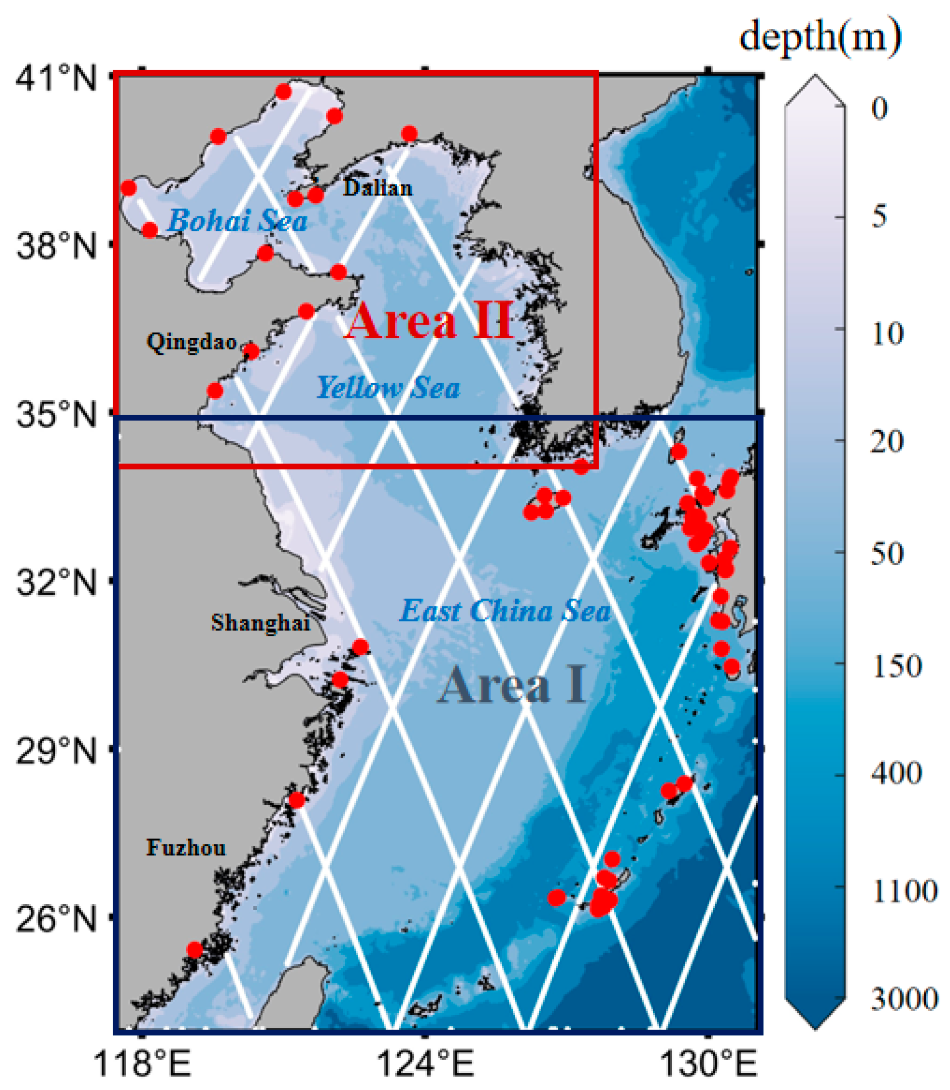
2.1. Study Region and Data
2.2. Methods
3. Results
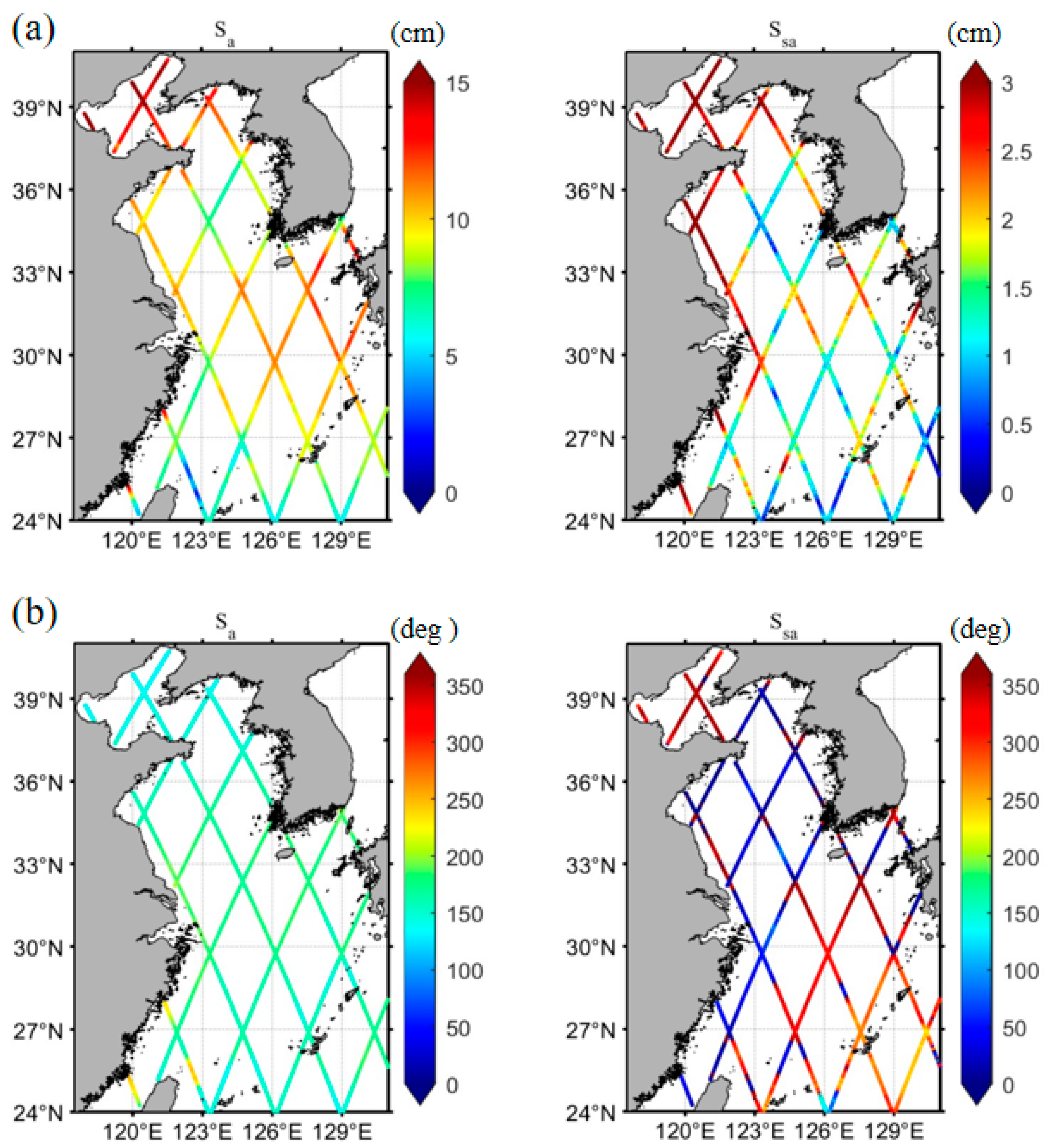
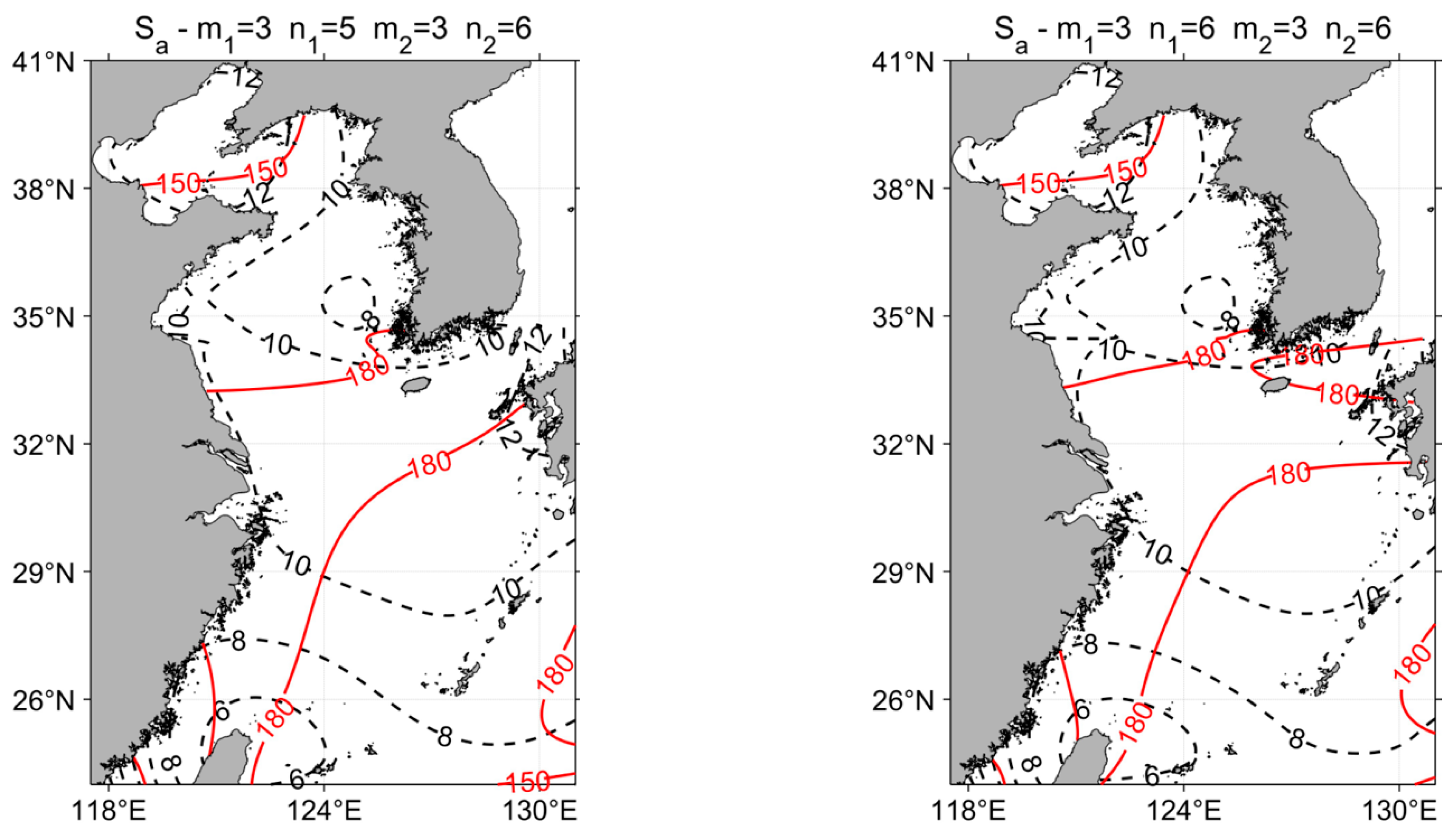
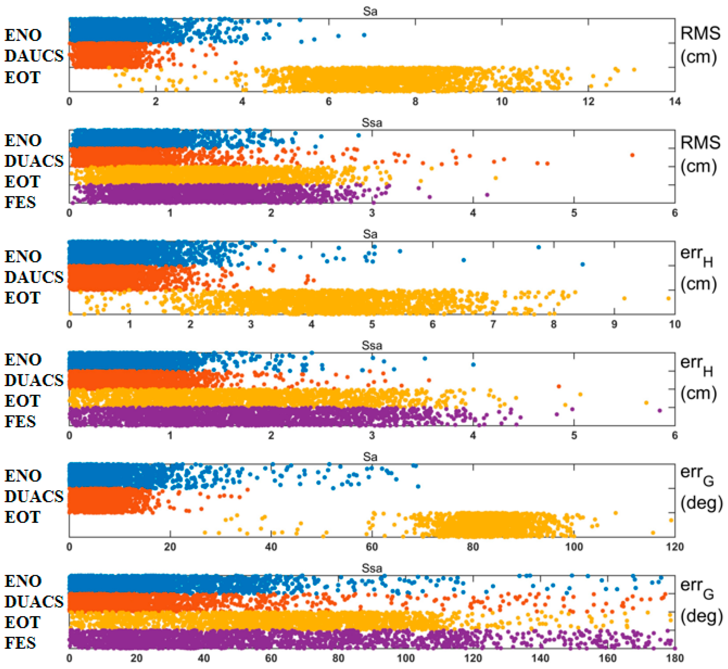
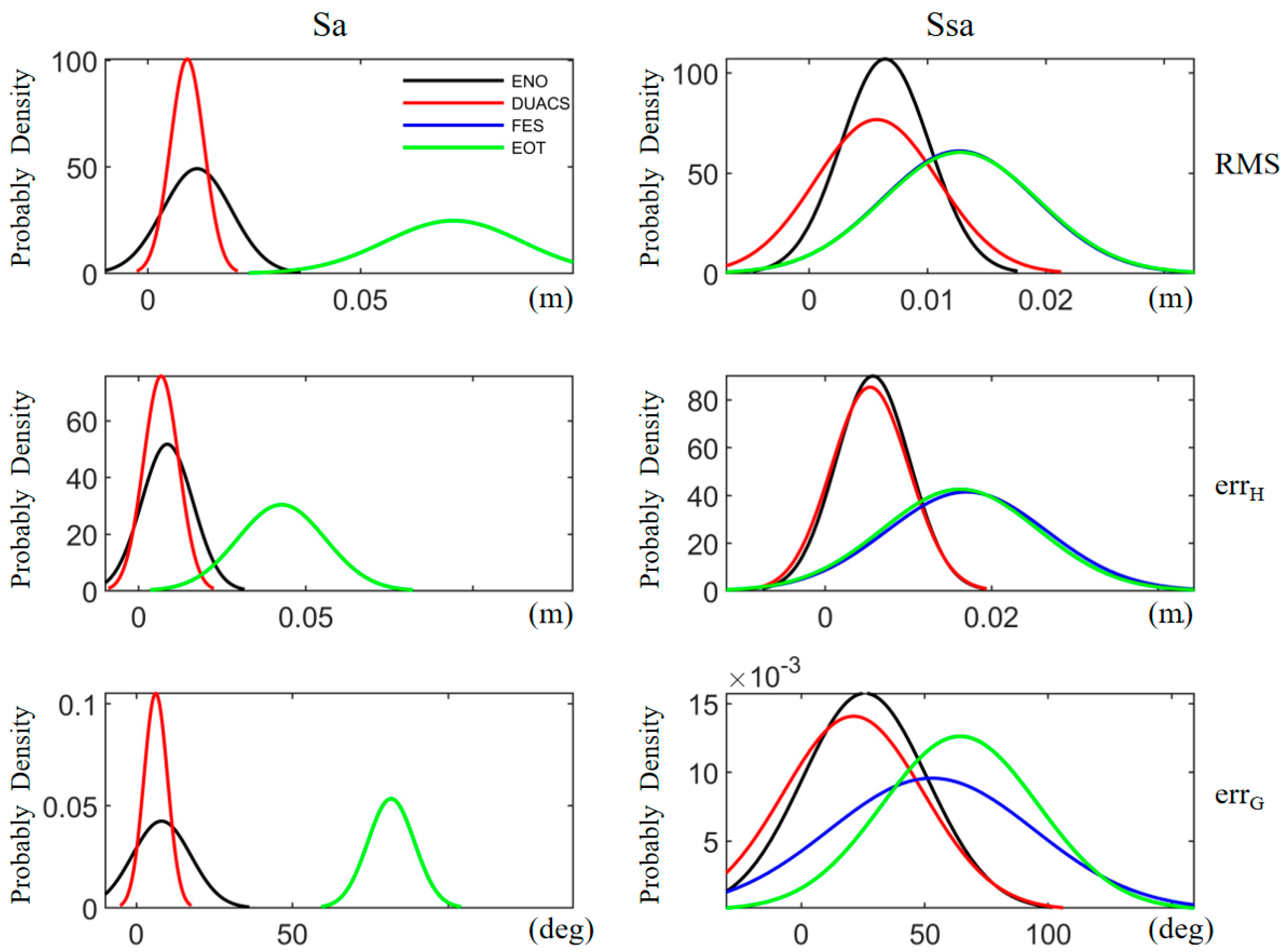
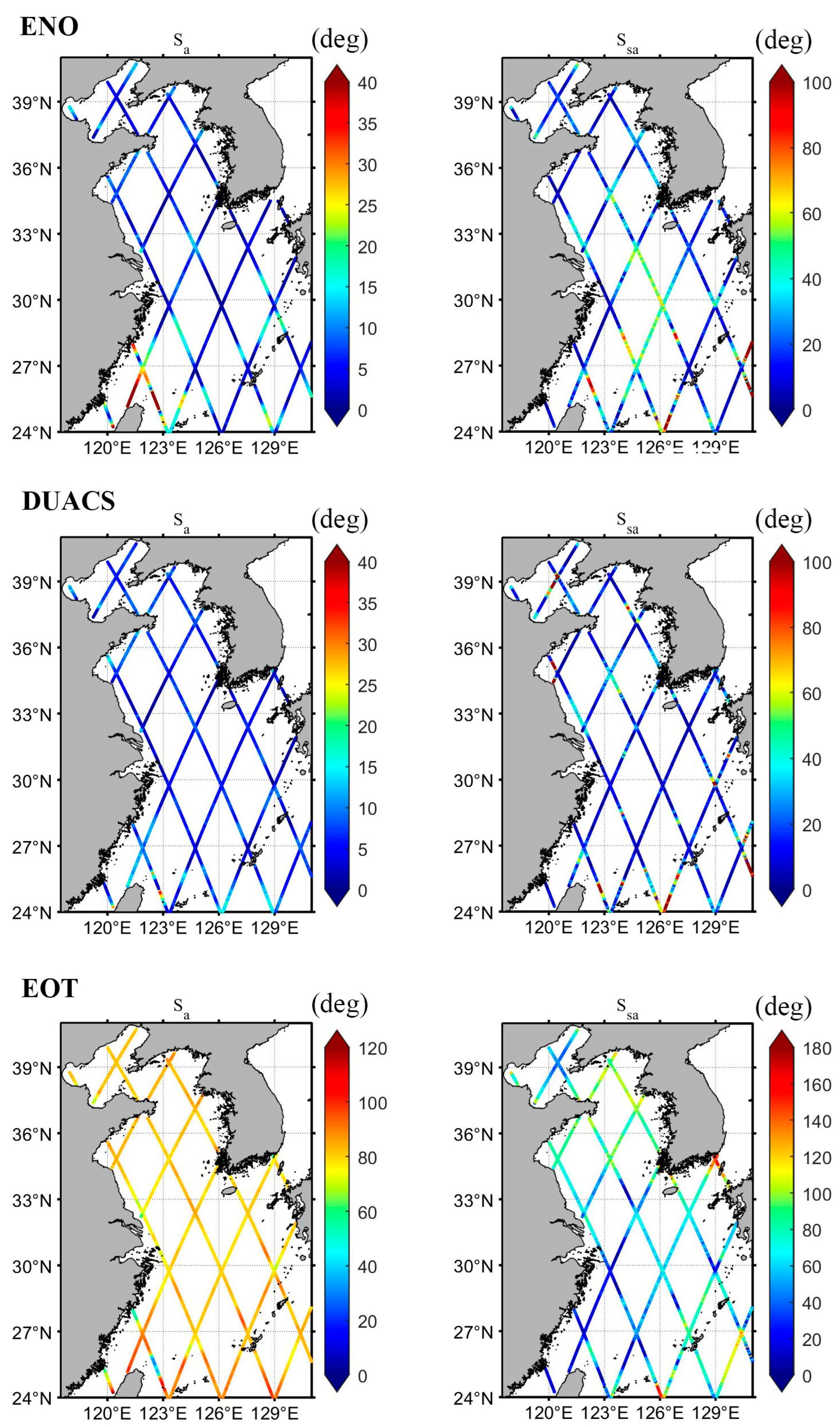
3.1. Comparison between Fitted Results and Orbit Data
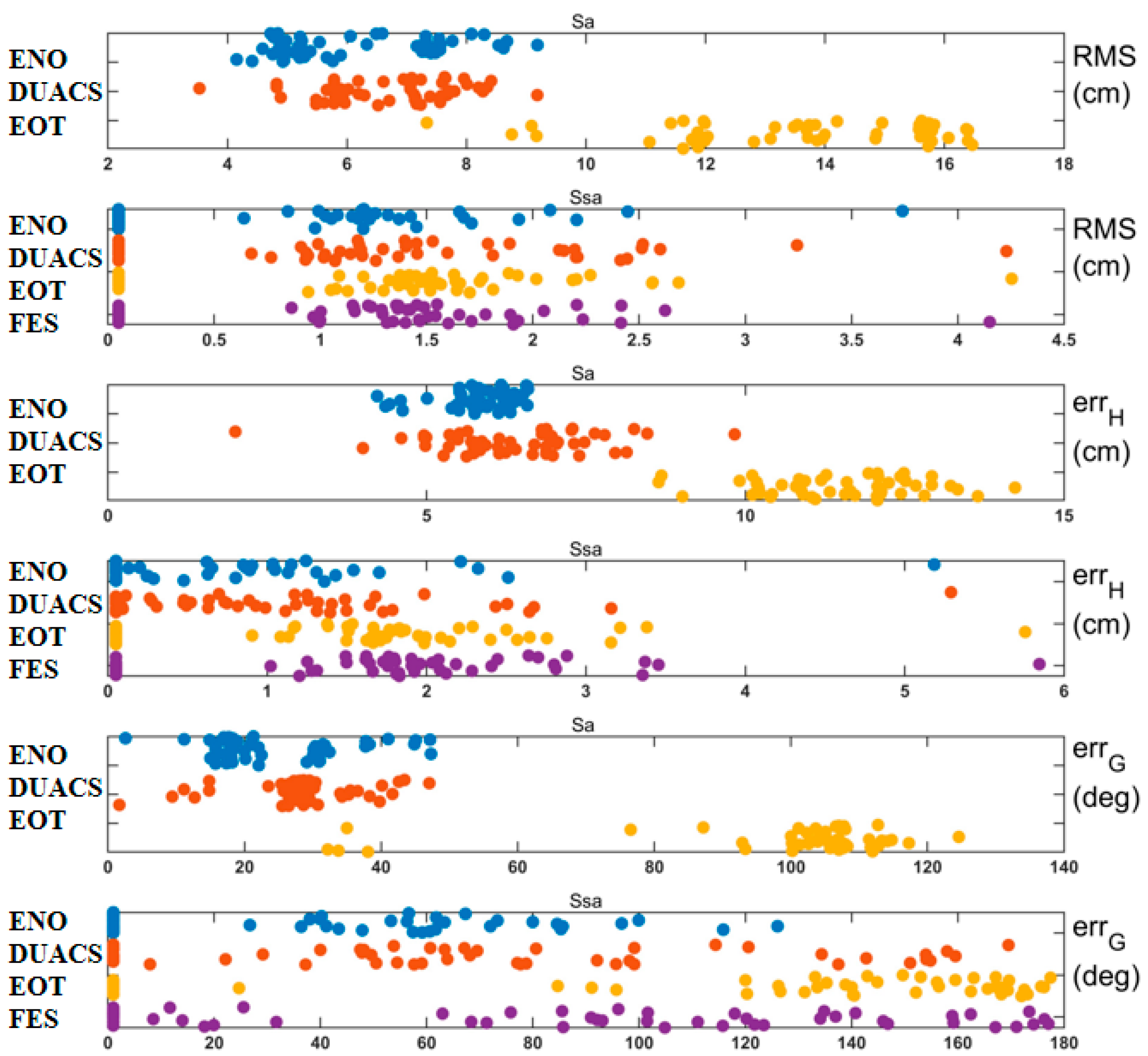
3.2. Comparison between Fitted Results and the Tide Gauges
4. Discussion
5. Conclusions
Author Contributions
Funding
Data Availability Statement
Acknowledgments
Conflicts of Interest
References
- Munk, W.; Wunsch, C. Abyssal Recipes II: Energetics of Tidal and Wind Mixing. Deep. Sea Res. Part I Oceanogr. Res. Pap. 1998, 45, 1977–2010. [Google Scholar] [CrossRef]
- Cook, S.E.; Lippmann, T.C.; Irish, J.D. Modeling Nonlinear Tidal Evolution in an Energetic Estuary. Ocean Model. 2019, 136, 13–27. [Google Scholar] [CrossRef]
- Fang, G. Dissipation of Tidal Energy in Yellow Sea. Oceanol. Limnol. Sin. 1979, 10, 200–213. [Google Scholar]
- Haigh, I.D.; Pickering, M.D.; Green, J.A.M.; Arbic, B.K.; Arns, A.; Dangendorf, S.; Hill, D.F.; Horsburgh, K.; Howard, T.; Idier, D.; et al. The Tides They Are A-Changin’: A Comprehensive Review of Past and Future Nonastronomical Changes in Tides, Their Driving Mechanisms, and Future Implications. Rev. Geophys. 2020, 58, e2018RG000636. [Google Scholar] [CrossRef] [Green Version]
- Bu, J.; Yu, K.; Park, H.; Huang, W.; Han, S.; Yan, Q.; Qian, N.; Lin, Y. Estimation of Swell Height Using Spaceborne GNSS-R Data from Eight CYGNSS Satellites. Remote Sens. 2022, 14, 4634. [Google Scholar] [CrossRef]
- Li, W.; Cardellach, E.; Fabra, F.; Ribo, S.; Rius, A. Assessment of Spaceborne GNSS-R Ocean Altimetry Performance Using CYGNSS Mission Raw Data. IEEE Trans. Geosci. Remote Sens. 2020, 58, 238–250. [Google Scholar] [CrossRef]
- Peng, Q.; Jin, S. Significant Wave Height Estimation from Space-Borne Cyclone-GNSS Reflectometry. Remote Sens. 2019, 11, 584. [Google Scholar] [CrossRef] [Green Version]
- Guillou, N.; Chapalain, G. Numerical Simulation of Tide-Induced Transport of Heterogeneous Sediments in the English Channel. Cont. Shelf Res. 2010, 30, 806–819. [Google Scholar] [CrossRef] [Green Version]
- Bao, X.; Gao, G.; Yan, J. Three Dimensional Simulation of Tide and Tidal Current Characteristics in the East China Sea. Oceanol. Acta 2001, 24, 135–149. [Google Scholar] [CrossRef] [Green Version]
- Niwa, Y.; Hibiya, T. Three-Dimensional Numerical Simulation of M2 Internal Tides in the East China Sea. J. Geophys. Res. Ocean. 2004, 109. [Google Scholar] [CrossRef]
- Cao, A.; Guo, Z.; Lü, X. Inversion of Two-Dimensional Tidal Open Boundary Conditions of M2 Constituent in the Bohai and Yellow Seas. Chin. J. Oceanol. Limnol. 2012, 30, 868–875. [Google Scholar] [CrossRef]
- Teng, F.; Fang, G.; Xu, X. Effects of Internal Tidal Dissipation and Self-Attraction and Loading on Semidiurnal Tides in the Bohai Sea, Yellow Sea and East China Sea: A Numerical Study. Chin. J. Oceanol. Limnol. 2017, 35, 987–1001. [Google Scholar] [CrossRef]
- Guo, X.; Yanagi, T. Three-Dimensional Structure of Tidal Current in the East China Sea and the Yellow Sea. J. Oceanogr. 1998, 54, 651–668. [Google Scholar] [CrossRef]
- Zheng, J.; Mao, X.; Lv, X.; Jiang, W. The M2 Cotidal Chart in the Bohai, Yellow, and East China Seas from Dynamically Constrained Interpolation. J. Atmos. Ocean. Technol. 2020, 37, 1219–1229. [Google Scholar] [CrossRef]
- Kuh Kang, S.; Lee, S.-R.; Lie, H.-J. Fine Grid Tidal Modeling of the Yellow and East China Seas. Cont. Shelf Res. 1998, 18, 739–772. [Google Scholar] [CrossRef]
- Andersen, O.B. Shallow Water Tides in the Northwest European Shelf Region from TOPEX/POSEIDON Altimetry. J. Geophys. Res. Oceans 1999, 104, 7729–7741. [Google Scholar] [CrossRef]
- He, Y.; Lu, X.; Qiu, Z.; Zhao, J. Shallow Water Tidal Constituents in the Bohai Sea and the Yellow Sea from a Numerical Adjoint Model with TOPEX/POSEIDON Altimeter Data. Cont. Shelf Res. 2004, 24, 1521–1529. [Google Scholar] [CrossRef]
- Gill, S.K.; Schultz, J.R. (Eds.) Tidal Datums and Their Applications; NOAA Special Publication NOS CO-OPS 1; NOAA, NOS Center for Operational Oceanographic Products and Services: Silver Spring, MD, USA, 2000. [CrossRef]
- Guohong, F. Tide and tidal current charts for the marginal seas adjacent to China. Chin. J. Oceanol. Limnol. 1986, 4, 1–16. [Google Scholar] [CrossRef]
- Smith, A.J.E.; Ambrosius, B.A.C.; Wakker, K.F.; Woodworth, P.L.; Vassie, J.M. Ocean tides from harmonic and response analysis on TOPEX/POSEIDON altimetry. Adv. Space Res. 1998, 22, 1541–1548. [Google Scholar] [CrossRef]
- Piccioni, G.; Dettmering, D.; Schwatke, C.; Passaro, M.; Seitz, F. Design and Regional Assessment of an Empirical Tidal Model Based on FES2014 and Coastal Altimetry. Adv. Space Res. 2021, 68, 1013–1022. [Google Scholar] [CrossRef]
- Deng, X.; Featherstone, W.E. A Coastal Retracking System for Satellite Radar Altimeter Waveforms: Application to ERS-2 around Australia. J. Geophys. Res. Oceans 2006, 111. [Google Scholar] [CrossRef] [Green Version]
- Roblou, L.; Lyard, F.; le Henaff, M.; Maraldi, C. X-Track, a New Processing Tool for Altimetry in Coastal Oceans. In Proceedings of the International Geoscience and Remote Sensing Symposium (IGARSS), Barcelona, Spain, 23–28 July 2007; pp. 5129–5133. [Google Scholar]
- Birol, F.; Léger, F.; Passaro, M.; Cazenave, A.; Niño, F.; Calafat, F.M.; Shaw, A.; Legeais, J.F.; Gouzenes, Y.; Schwatke, C.; et al. The X-TRACK/ALES Multi-Mission Processing System: New Advances in Altimetry towards the Coast. Adv. Space Res. 2021, 67, 2398–2415. [Google Scholar] [CrossRef]
- Lyard, F.H.; Allain, D.J.; Cancet, M.; Carrère, L.; Picot, N. FES2014 Global Ocean Tide Atlas: Design and Performance. Ocean. Sci. 2021, 17, 615–649. [Google Scholar] [CrossRef]
- Hart-Davis, M.G.; Piccioni, G.; Dettmering, D.; Schwatke, C.; Passaro, M.; Seitz, F. EOT20: A Global Ocean Tide Model from Multi-Mission Satellite Altimetry. Earth Syst. Sci. Data 2021, 13, 3869–3884. [Google Scholar] [CrossRef]
- Ray, R.D.; Erofeeva, S.Y. Long-Period Tidal Variations in the Length of Day. J. Geophys. Res. Solid Earth 2014, 119, 1498–1509. [Google Scholar] [CrossRef]
- Cartwright, D.E.; Tayler, R.J. New Computations of the Tide-generating Potential. Geophys. J. R. Astron. Soc. 1971, 23, 45–73. [Google Scholar] [CrossRef] [Green Version]
- Woodworth, P.L. A Note on the Nodal Tide in Sea Level Records. J. Coast. Res. 2012, 28, 316–323. [Google Scholar] [CrossRef] [Green Version]
- Ponte, R.M.; Chaudhuri, A.H.; Vinogradov, S.V. Long-Period Tides in an Atmospherically Driven, Stratified Ocean. J. Phys. Oceanogr. 2015, 45, 1917–1928. [Google Scholar] [CrossRef]
- Kantha, L.H.; Stewart, J.S.; Desai, S.D. Long-Period Lunar Fortnightly and Monthly Ocean Tides. J. Geophys. Res. Oceans 1998, 103, 12639–12647. [Google Scholar] [CrossRef]
- Wunsch, C.; Haidvogel, D.B.; Iskandarani, M.; Hughes, R. Dynamics of the Long-Period Tides. Prog. Oceanogr. 1997, 40, 81–108. [Google Scholar] [CrossRef]
- Lee, E.J.; Kim, K.; Park, J.H. Reconstruction of Long-Term Sea-Level Data Gaps of Tide Gauge Records Using a Neural Network Operator. Front. Mar. Sci. 2022, 9, 1037697. [Google Scholar] [CrossRef]
- Xu, M.; Wang, Y.; Wang, S.; Lv, X.; Chen, X. Ocean Tides near Hawaii from Satellite Altimeter Data. Part I. J. Atmos. Ocean. Technol. 2021, 38, 937–949. [Google Scholar] [CrossRef]
- Wang, Q.; Zhang, Y.; Wang, Y.; Xu, M.; Lv, X. Fitting Cotidal Charts of Eight Major Tidal Components in the Bohai Sea, Yellow Sea Based on Chebyshev Polynomial Method. J. Mar. Sci. Eng. 2022, 10, 1219. [Google Scholar] [CrossRef]
- Wang, Y.; Zhang, Y.; Xu, M.; Wang, Y.; Lv, X. Ocean Tides near Hawaii from Satellite Altimeter Data. Part II. J. Atmos. Ocean Technol. 2022, 39, 1015–1029. [Google Scholar] [CrossRef]
- Romero, M.; de Madrid, A.P.; Mañoso, C.; Vinagre, B.M. IIR Approximations to the Fractional Differentiator/Integrator Using Chebyshev Polynomials Theory. ISA Trans. 2013, 52, 461–468. [Google Scholar] [CrossRef] [PubMed]
- Hu, X.-Y.; Yu, X.-H. The Chebyshev Polynomial Fitting Properties of Discrete Cosine Transform. Signal Process. Image Commun. 1998, 13, 15–20. [Google Scholar] [CrossRef]


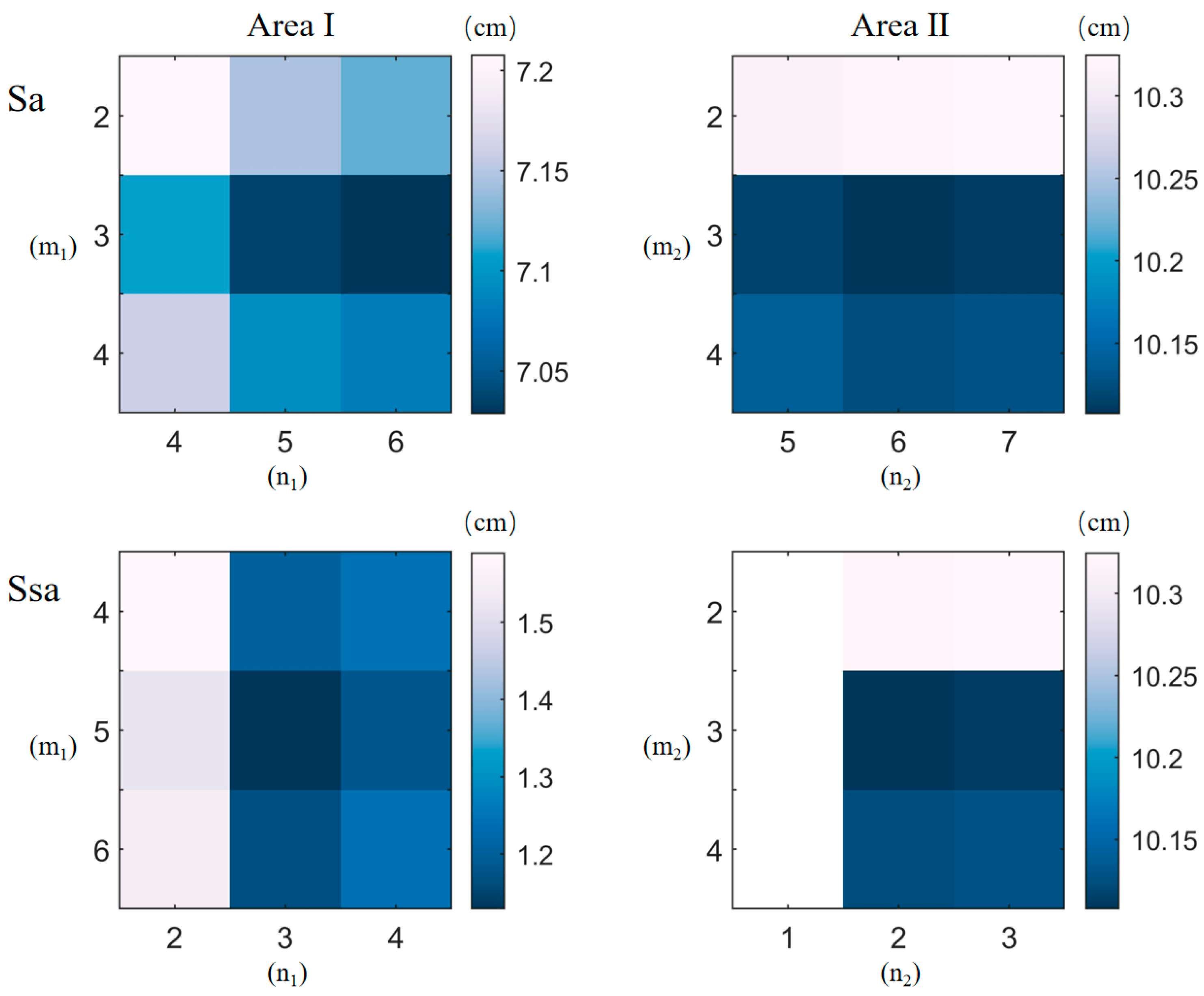
| Sa (cm) | m2 = 3 n2 = 5 | m2 = 3 n2 = 6 | m2 = 3 n2 = 7 |
| m1 = 3 n1 = 5 | 0.66 | 0.62 | 0.68 |
| m1 = 3 n1 = 6 | 0.69 | 0.70 | 0.70 |
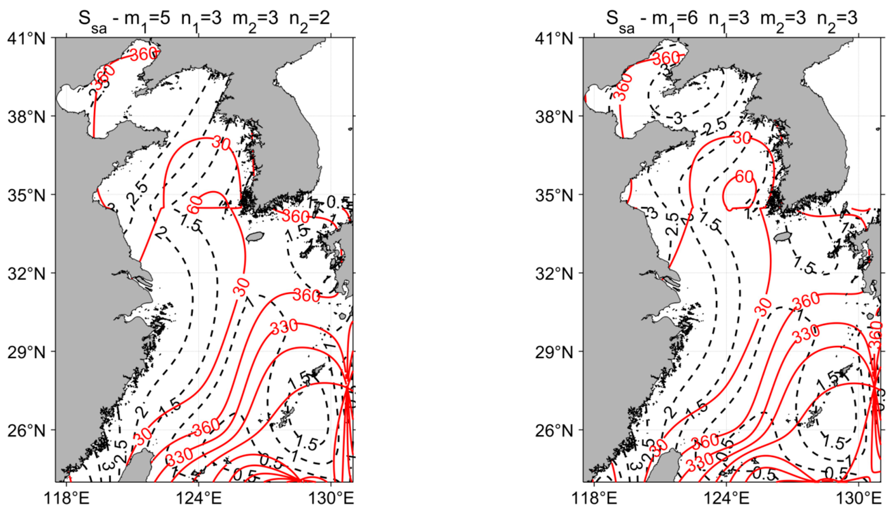
| Ssa (cm) | m1 = 5 n1 = 3 | m1 = 5 n1 = 4 | m1 = 6 n1 = 3 |
| m2 = 3 n2 = 2 | 0.21 | 0.46 | 0.48 |
| m2 = 3 n2 = 3 | 0.27 | 0.27 | 0.21 |
| Area I | Sa | Ssa | Area II | Sa | Ssa |
|---|---|---|---|---|---|
| m1 | 3 | 5 | m1 | 3 | 3 |
| n1 | 5 | 3 | n2 | 6 | 2 |
| RMSE (cm) | ENOPF | DUACS | FES2014 | EOT20 |
| 1.15 | 0.93 | / | 7.19 | |
| 0.64 | 0.57 | 1.27 | 1.28 | |
| (cm) | ENOPF | DUACS | FES2014 | EOT20 |
| 0.85 | 0.67 | / | 4.27 | |
| 0.57 | 0.54 | 1.70 | 1.62 | |
| (deg) | ENOPF | DUACS | FES2014 | EOT20 |
| 8.03 | 6.16 | / | 81.63 | |
| 25.91 | 21.14 | 52.88 | 64.36 |
| RMSE (cm) | ENOPF | DUACS | FES2014 | EOT20 |
| 6.19 | 6.85 | / | 13.53 | |
| 1.10 | 1.21 | 1.24 | 1.34 | |
| (cm) | ENOPF | DUACS | FES2014 | EOT20 |
| 5.85 | 6.44 | / | 11.55 | |
| 0.72 | 0.83 | 1.69 | 1.55 | |
| (deg) | ENOPF | DUACS | FES2014 | EOT20 |
| 25.44 | 28.79 | / | 101.41 | |
| 59.09 | 76.16 | 107.56 | 150.88 |
Disclaimer/Publisher’s Note: The statements, opinions and data contained in all publications are solely those of the individual author(s) and contributor(s) and not of MDPI and/or the editor(s). MDPI and/or the editor(s) disclaim responsibility for any injury to people or property resulting from any ideas, methods, instructions or products referred to in the content. |
© 2023 by the authors. Licensee MDPI, Basel, Switzerland. This article is an open access article distributed under the terms and conditions of the Creative Commons Attribution (CC BY) license (https://creativecommons.org/licenses/by/4.0/).
Share and Cite
Zhang, Y.; Wang, Q.; Zhang, Y.; Xu, M.; Wang, Y.; Lv, X. Equidistant Nodes Orthogonal Polynomial Fitting for Harmonic Constants of Long-Period Tides Based on Satellite Altimeter Data. Remote Sens. 2023, 15, 3246. https://doi.org/10.3390/rs15133246
Zhang Y, Wang Q, Zhang Y, Xu M, Wang Y, Lv X. Equidistant Nodes Orthogonal Polynomial Fitting for Harmonic Constants of Long-Period Tides Based on Satellite Altimeter Data. Remote Sensing. 2023; 15(13):3246. https://doi.org/10.3390/rs15133246
Chicago/Turabian StyleZhang, Yunfei, Qixiang Wang, Yibo Zhang, Minjie Xu, Yonggang Wang, and Xianqing Lv. 2023. "Equidistant Nodes Orthogonal Polynomial Fitting for Harmonic Constants of Long-Period Tides Based on Satellite Altimeter Data" Remote Sensing 15, no. 13: 3246. https://doi.org/10.3390/rs15133246