
A Novel Method to Improve the Estimation of Ocean Tide Loading Displacements for K1 and K2 Components with GPS Observations

Abstract
:1. Introduction
2. Methodology and Data
3. Results and Discussions
3.1. Results
3.2. Discussions: The Advantages and Limitations of the Proposed Methodology
4. Conclusions
Funding
Data Availability Statement
Conflicts of Interest
Appendix A


References
- Ray, R.D. On Tidal Inference in the Diurnal Band. J. Atmos. Ocean. Technol. 2017, 34, 437–446. [Google Scholar] [CrossRef]
- Gan, M.; Pan, H.; Chen, Y.; Pan, S. Application of the Variational Mode Decomposition (VMD) Method to River Tides. Estuar. Coast. Shelf Sci. 2021, 261, 107570. [Google Scholar] [CrossRef]
- Wei, Z.; Pan, H.; Xu, T.; Wang, Y.; Wang, J. Development History of the Numerical Simulation of Tides in the East Asian Marginal Seas: An Overview. J. Mar. Sci. Eng. 2022, 10, 984. [Google Scholar] [CrossRef]
- Zhou, M.; Liu, X.; Yuan, J.; Jin, X.; Niu, Y.; Guo, J.; Gao, H. Seasonal Variation of GPS-Derived the Principal Ocean Tidal Constituents’ Loading Displacement Parameters Based on Moving Harmonic Analysis in Hong Kong. Remote Sens. 2021, 13, 279. [Google Scholar] [CrossRef]
- Yuan, L.; Chao, B.F.; Ding, X.; Zhong, P. The tidal displacement field at Earth’ s surface determined using global GPS observations. J. Geophys. Res. Solid Earth 2013, 118, 2618–2632. [Google Scholar] [CrossRef]
- Wei, G.; Chen, K.; Ji, R. Improving estimates of ocean tide loading displacements with multi-GNSS: A case study of Hong Kong. GPS Solut. 2022, 26, 25. [Google Scholar] [CrossRef]
- Farrell, W. Deformation of the Earth by surface loads. Rev. Geophys. 1972, 10, 761–797. [Google Scholar] [CrossRef]
- Francis, O.; Mazzega, P. Global charts of ocean tide loading effects. J. Geophys. Res. 1990, 95, 11411–11424. [Google Scholar] [CrossRef]
- Hart-Davis, M.; Piccioni, G.; Dettmering, D.; Schwatke, C.; Passaro, M.; Seitz, F. EOT20: A global ocean tide model from multi-mission satellite altimetry. Earth Syst. Sci. Data. 2021, 13, 3869–3884. [Google Scholar] [CrossRef]
- Wei, G.; Wang, Q.; Peng, W. Accurate evaluation of vertical tidal displacement determined by GPS kinematic precise point positioning: A case study of Hong Kong. Sensors 2019, 19, 2559. [Google Scholar] [CrossRef]
- Abbaszadeh, M.; Clarke, P.; Penna, N. Benefits of combining GPS and GLONASS for measuring ocean tide loading displacement. J Geod. 2020, 94, 63. [Google Scholar] [CrossRef]
- Munk, W.H.; Cartwright, D.E. Tidal spectroscopy and prediction. Philos. Trans. R. Soc. London A 1966, 259, 533–581. [Google Scholar]
- Feng, X.; Tsimplis, M.; Woodworth, P. Nodal variations and long-term changes in the main tides on the coasts of China. J. Geophys. Res. Ocean. 2015, 120, 1215–1232. [Google Scholar] [CrossRef]
- Pan, H.; Xu, T.; Wei, Z. Anomalously large seasonal modulations of shallow water tides at Lamu, Kenya. Estuar. Coast. Shelf Sci. 2023, 281, 108203. [Google Scholar] [CrossRef]
- Pan, H.; Lv, X.; Wang, Y.; Matte, P.; Chen, H.; Jin, G. Exploration of Tidal-Fluvial Interaction in the Columbia River Estuary Using S_TIDE. J. Geophys. Res. Ocean. 2018, 123, 6598–6619. [Google Scholar] [CrossRef]
- Pan, H.; Zheng, Q.; Lv, X. Temporal changes in the response of the nodal modulation of the M2 tide in the Gulf of Maine. Cont. Shelf Res. 2019, 186, 13–20. [Google Scholar] [CrossRef]
- Pan, H.; Lv, X. Is There a Quasi 60-Year Oscillation in Global Tides? Cont. Shelf Res. 2021, 222, 104433. [Google Scholar] [CrossRef]
- Lyard, F.; Allain, D.; Cancet, M.; Carrère, L.; Picot, N. FES2014 global ocean tide atlas: Design and performance. Ocean. Sci. 2021, 17, 615–649. [Google Scholar] [CrossRef]
- Pan, H.; Devlin, A.T.; Xu, T.; Lv, X.; Wei, Z. Anomalous 18.61-Year Nodal Cycles in the Gulf of Tonkin Revealed by Tide Gauges and Satellite Altimeter Records. Remote Sens. 2022, 14, 3672. [Google Scholar] [CrossRef]
- Cartwright, D.E.; Ray, R.D. On the radiational anomaly in the global ocean tide with reference to satellite altimetry. Oceanol. Acta. 1994, 17, 453–459. [Google Scholar]
- Fang, G.; Xu, X.; Wei, Z.; Wang, Y.; Wang, X. Vertical displacement loading tides and self-attraction and loading tides in the Bohai, Yellow, and East China Seas. Sci. China Earth Sci. 2013, 56, 63–70. [Google Scholar] [CrossRef]
- Bos, M.; Penna, N.; Baker, T.; Clarke, P. Ocean tide loading displacements in western Europe: 2. GPS -observed anelastic dispersion in the asthenosphere. J. Geophys. Res. Solid Earth. 2015, 120, 6523–6539. [Google Scholar] [CrossRef]
- Yuan, L.; Ding, X.; Sun, H.; Zhong, P.; Chen, W. Determination of ocean tide loading displacements in Hong Kong using GPS technique. Sci. China Earth Sci. 2010, 53, 993–1007. [Google Scholar] [CrossRef]
- Zetler, B.D. Radiational ocean tides along the coasts of the United States. J. Phys. Oceanogr. 1971, 1, 34–38. [Google Scholar] [CrossRef]
- Zhang, X.; Li, X. Satellite data-driven and knowledge-informed machine learning model for estimating global internal solitary wave speed. Remote Sens. Environ. 2022, 283, 113328. [Google Scholar] [CrossRef]
- Li, X.; Liu, B.; Zheng, G.; Ren, Y.; Zhang, S.; Liu, Y.; Gao, L.; Liu, Y.; Zhang, B.; Wang, F. Deep-learning-based information mining from ocean remote-sensing imagery. Natl. Sci. Rev. 2020, 7, 1584–1605. [Google Scholar] [CrossRef]


| Tide | Period/Hour | Eq Amp | U Amp | U Pha | N Amp | N Pha | E Amp | E Pha |
|---|---|---|---|---|---|---|---|---|
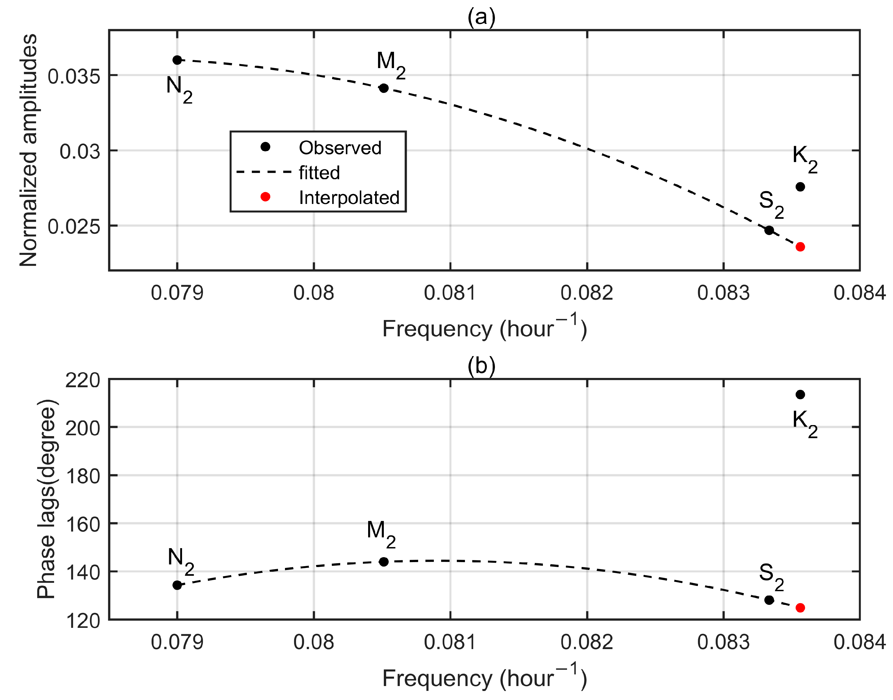
| M2 | 12.421 | 121.29 | 14.51 | 122.7 | 4.14 | 144.0 | 3.77 | 219.1 |
| S2 | 12.000 | 56.31 | 8.33 | 146.6 | 1.39 | 128.1 | 2.17 | 223.6 |
| N2 | 12.658 | 23.61 | 3.01 | 118.0 | 0.85 | 134.3 | 0.66 | 207.8 |
| K2 | 11.967 | 15.59 | 2.70 | 115.2 | 0.43 | 213.5 | 0.15 | 175.2 |
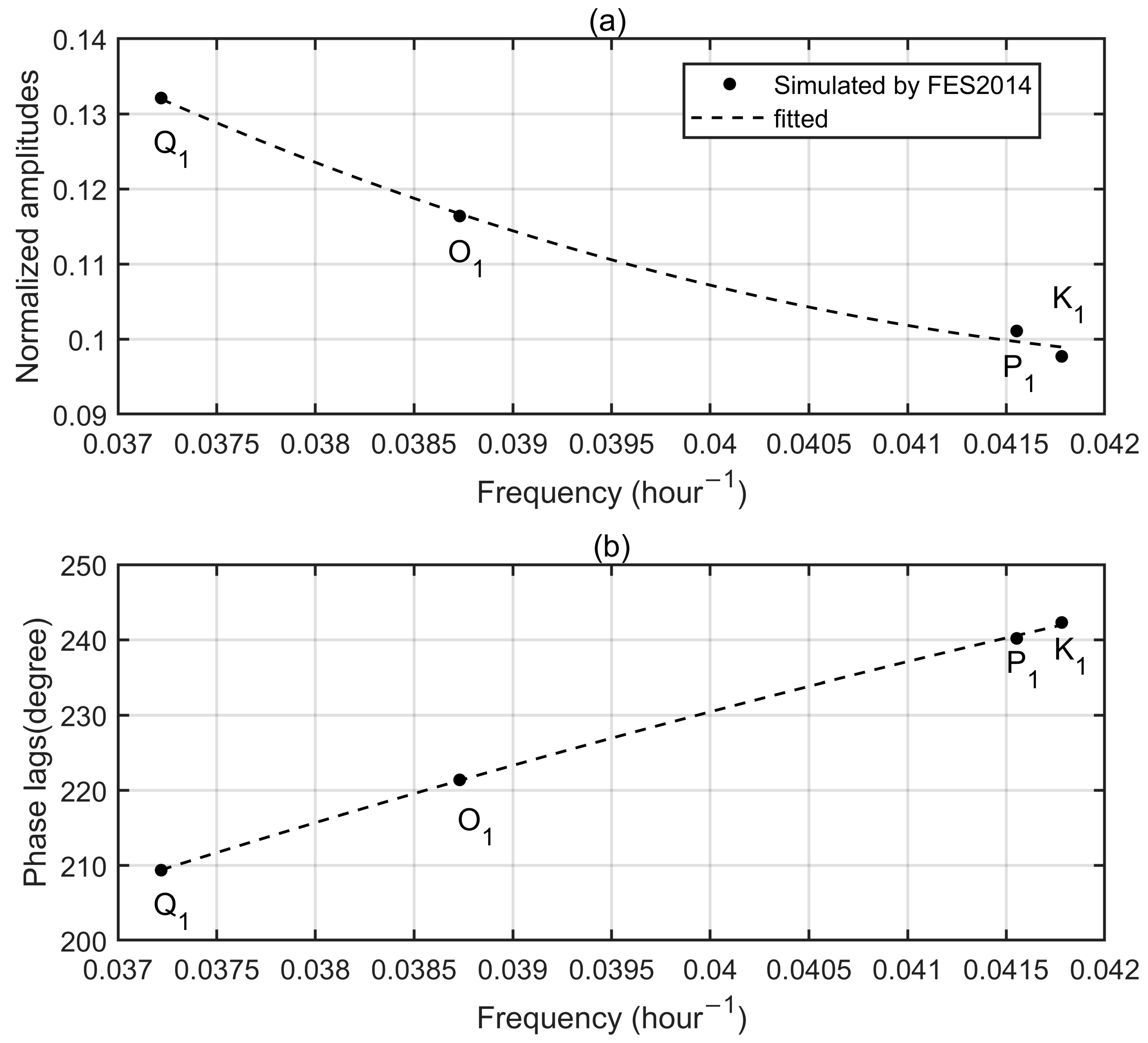
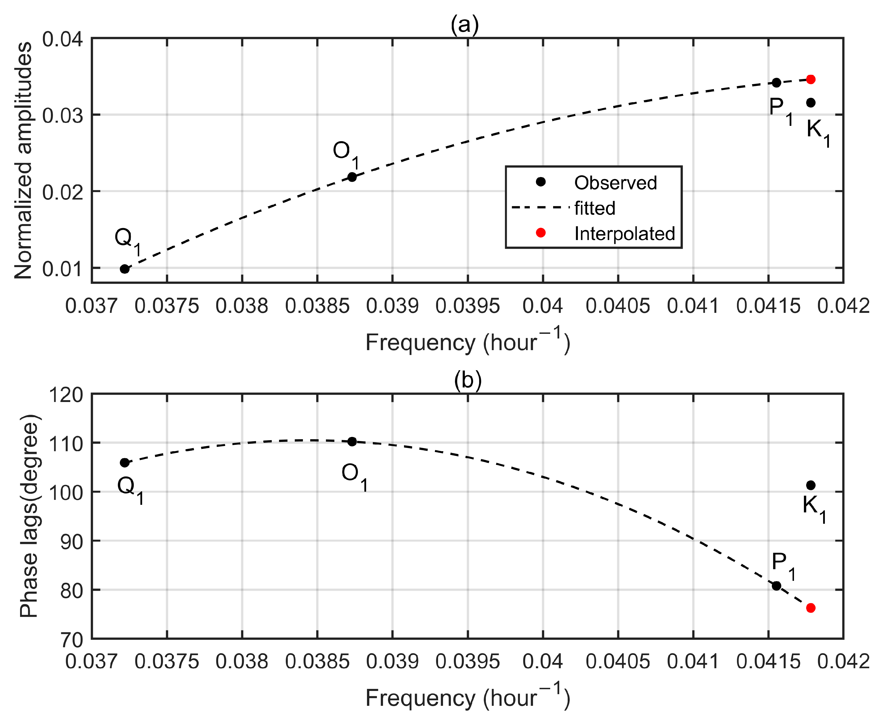
| K1 | 23.934 | 93.19 | 9.85 | 228.4 | 2.94 | 101.3 | 3.68 | 29.3 |
| O1 | 25.819 | 62.73 | 7.71 | 224.7 | 1.37 | 110.2 | 3.02 | 10.6 |
| P1 | 24.066 | 29.57 | 3.24 | 242.4 | 1.01 | 80.8 | 1.23 | 39.1 |
| Q1 | 26.868 | 12.19 | 1.66 | 211.4 | 0.12 | 105.9 | 0.57 | 3.2 |
Disclaimer/Publisher’s Note: The statements, opinions and data contained in all publications are solely those of the individual author(s) and contributor(s) and not of MDPI and/or the editor(s). MDPI and/or the editor(s) disclaim responsibility for any injury to people or property resulting from any ideas, methods, instructions or products referred to in the content. |
© 2023 by the authors. Licensee MDPI, Basel, Switzerland. This article is an open access article distributed under the terms and conditions of the Creative Commons Attribution (CC BY) license (https://creativecommons.org/licenses/by/4.0/).
Share and Cite
Pan, H.; Xu, X.; Zhang, H.; Xu, T.; Wei, Z. A Novel Method to Improve the Estimation of Ocean Tide Loading Displacements for K1 and K2 Components with GPS Observations. Remote Sens. 2023, 15, 2846. https://doi.org/10.3390/rs15112846
Pan H, Xu X, Zhang H, Xu T, Wei Z. A Novel Method to Improve the Estimation of Ocean Tide Loading Displacements for K1 and K2 Components with GPS Observations. Remote Sensing. 2023; 15(11):2846. https://doi.org/10.3390/rs15112846
Chicago/Turabian StylePan, Haidong, Xiaoqing Xu, Huayi Zhang, Tengfei Xu, and Zexun Wei. 2023. "A Novel Method to Improve the Estimation of Ocean Tide Loading Displacements for K1 and K2 Components with GPS Observations" Remote Sensing 15, no. 11: 2846. https://doi.org/10.3390/rs15112846