Two-Dimensional Numerical Simulation of Tide and Tidal Current of Eight Major Tidal Constituents in the Bohai, Yellow, and East China Seas

Abstract

Numerical simulations of the eight major tidal constituents (M₂, S₂, K₁, O₁, N₂, K₂, P₁, and Q₁) in the Bohai, Yellow and East China Seas (BYES) were conducted using the Regional Ocean Modeling System (ROMS) based on altimeter products from X-TRACK. Tidal harmonic constants and two-dimensional tidal current data with a spatial resolution of 1/12° were obtained. To validate the simulation results (SRs), harmonic constants from altimeters and tide gauges, two sea level anomaly time series, and velocity observations from 12 current meters were utilized. Additionally, data from five tidal models were used for comparison. The validation and comparison results demonstrated the accuracy of SR, especially when compared with coastal tide gauge data where SR performs exceptionally well. The cotidal charts and tidal current ellipses obtained through SR exhibited good continuity and consistency with the previous studies, effectively reflecting the tidal characteristics of the BYES. The SR can serve as a valuable reference and support for tidal-related fields in the BYES, including the supplement and verification of ocean measurements and the calculation of reference planes for ocean engineering.

1. Introduction

Tides are an important and fundamental component of ocean dynamics. The generation of internal waves by tides, known as internal tides, provides the majority of the mechanical energy necessary for maintaining internal turbulent mixing in the ocean, which has a significant impact on climate [1,2]. Tides and their interaction with storm surges and waves can strongly influence sea level in coastal areas, with implications for coastal engineering and the environment [3,4]. The cyclic variations in seawater properties induced by tidal currents can also affect the marine ecosystem [5]. Accurate understanding of tides is required in various fields of geophysics [6,7].

The Bohai, Yellow, and East China Seas (BYES) are typical marginal seas surrounded by land and islands with complex topography and tortuous coastlines. They are among the most active and complex regions in the world in terms of tides and tidal currents [8]. The diurnal and semi-diurnal tidal currents in the BYES have been calculated in the early two-dimensional numerical simulation, and the propagation and dissipation of tidal energy have been given [9,10]. However, it is difficult for two-dimensional numerical simulation to distinguish the vertical structure of tidal currents. The three-dimensional numerical model with high resolution can simulate the BYES more accurately [11,12]. Zhu et al. [12] used FVCOM to indicate that three diurnal and five semidiurnal constituents of independent rotary tidal systems appear in BYES, and they are all anti-clockwise. Twelve tidal current-amphidromic points for diurnal and semi-diurnal constituents are also given. Due to the complex coastline topography and water depth of BYES, it is necessary to have more precise and high-resolution data to effectively study tides in this area. The study of tides in the BYES is of great significance, and the tidal characteristics of the region have been systematically researched for a long time [13,14].

To effectively study tides in the BYES area, it is necessary to have more precise and high-resolution data due to the intricate nature of their complexity. The study of tides in the BYES is of great significance, and the tidal characteristics of the region have been systematically researched for a long time [13,14].

With the advancement of observation technology, satellite altimeters have been used to provide sea level anomaly (SLA) data. This has greatly improved the study of tides in various regions, including the BYES [15]. Altimetry data can be directly employed to depict the tidal characteristics of a region. Fang et al. [8] used 10 years of TOPEX/Poseidon (T/P) altimeter data to obtain empirical cotidal charts of the main diurnal, semidiurnal, and long-period constituents in BYES. Cotidal charts of various constituents near the Hawaiian were derived by fitting T/P altimeter data using Chebyshev polynomials fitting (CPF) [16,17,18]. The CPF method for processing altimeter data to obtain tidal harmonic constants has also been applied to the Bohai and Yellow Seas [19]. However, altimeter sampling exhibits spatial discontinuity, particularly in marginal seas with convoluted coastlines where data are dispersed and scarce. Simultaneously, satellite signals can be contaminated by land near the coast, which can diminish the accuracy of altimeter data in tidal research in coastal regions [20,21].

The development and utilization of tidal models can better characterize the tide in various regions and provide tide corrections for ocean measurements [7]. When performing numerical simulations on small-scale marginal seas, open boundary conditions (OBCs) are key parameters. In the case where there is a lack of observation in the region to derive OBCs, the required data must be obtained from model data. This places demands on the accuracy and resolution of the model data [22]. The deficiencies in altimeter observations require corresponding corrections. Tidal model data can be used to correct altimeter measurements, such as for satellite altimetry data correction [23]. The chart datum is a height reference surface used in hydrography and must be considered in activities, such as ship navigation and port construction [24]. Moreover, chart datum can facilitate accurate satellite navigation and offshore surveying [25]. Tides are one of the important factors in chart datum calculation. Accurate high-resolution ocean tidal model data play an indispensable role in the derivation of regional chart datums. Additionally, tidal models facilitate research on internal tides, storm surges, and ocean circulation [16].

Accurate and high-resolution tidal model data can provide great support and assistance for the study of tidal characteristics in China’s coastal areas, sea level and its long-term changes, calibration of new satellite altimeters, maritime transportation, and offshore engineering construction. This study employs the Regional Ocean Modeling System (ROMS) [26] model and X-TRACK altimeter data (2016 version) to conduct a numerical simulation of the eight major tidal constituents (M₂, S₂, K₁, O₁, N₂, K₂, P₁, and Q₁) in BYES. High-resolution two-dimensional tidal harmonic constants and tidal current data in the BYES are obtained.

Two key parameters in the model, the OBCs and bottom friction coefficients (BFCs), are obtained from altimeter data. The CPF method is used to directly fit the harmonic constants of satellite altimeter data to obtain OBCs. The CPF method has been validated for calculating the harmonic constants of eight major constituents and has demonstrated excellent performance in the area near Hawaii (open sea) and Bohai and Yellow Seas (marginal seas) [16,19]. The altimeter data are assimilated by the adjoint method to estimate BFCs. Lu and Zhang [27] used the adjoint method to assimilate T/P altimeter data and estimate the spatially varying BFCs of the M₂ tidal constituent in BYES. Gao et al. [28] optimized the BFCs in the South China Sea by assimilating T/P altimeter and tide gauge data using the adjoint method and numerically simulated the four tidal constituents M₂, S₂, K₁, and O₁. Wang et al. [29] utilized harmonic constants of the four tidal constituents (M₂, S₂, K₁, and O₁) derived from T/P altimeter data and employed the adjoint method to estimate the spatially and temporally varying BFCs in BYES. By combining the aforementioned technical means, tidal and tidal current data with a horizontal resolution of 5′ × 5′ are obtained. The simulated results (SRs) are evaluated using observational data from altimeters, tide gauges, and current meters. The results of five commonly used tidal models are also compared with SR to verify their effectiveness.

The paper is organized as follows. The data and methodology are introduced in Section 2. In Section 3, the SR are validated using altimeter, tide gauge data, and other observations, a comparison with five models is also included. Section 4 provides a summary and discussion.

2. Materials and Methodology

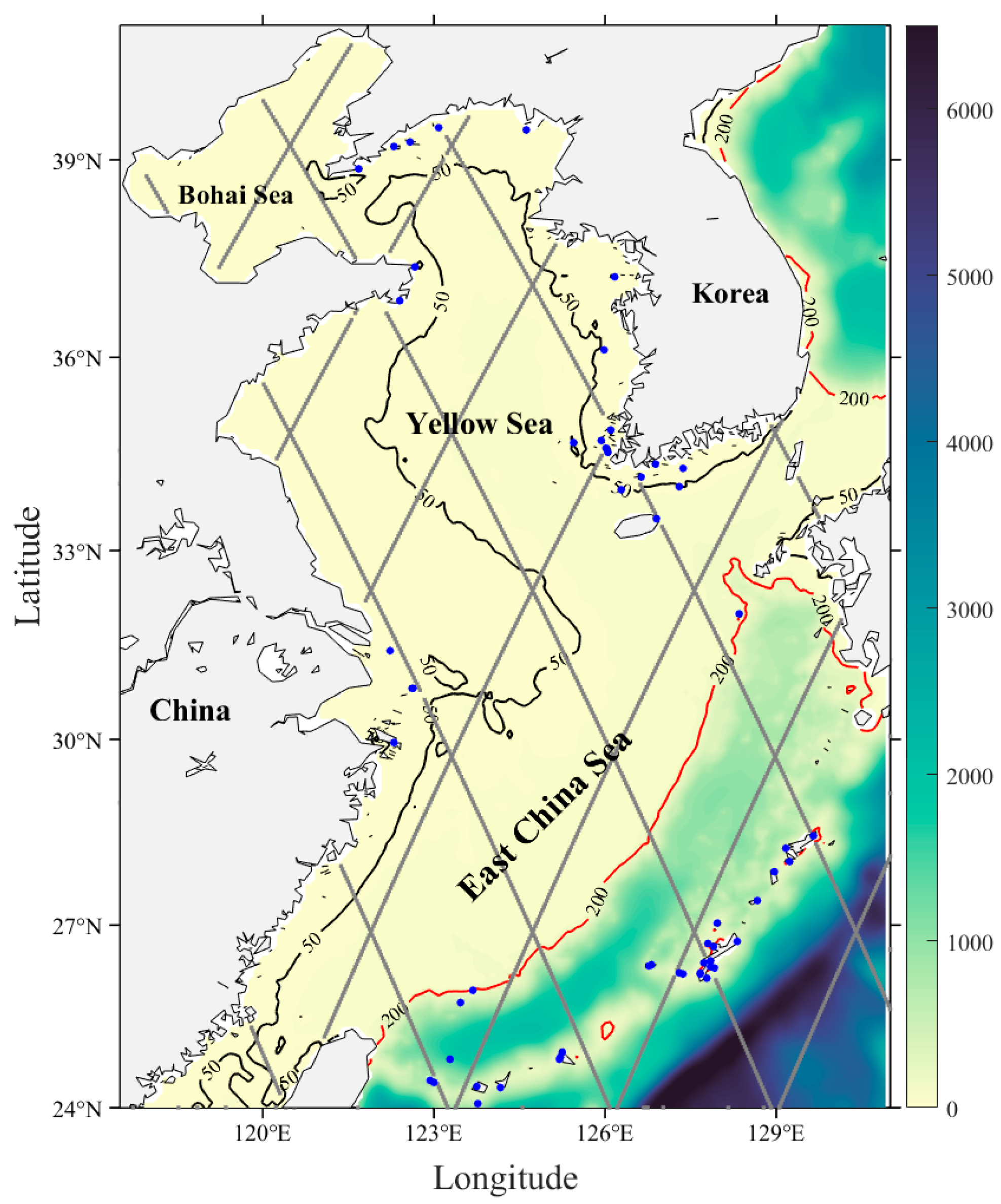
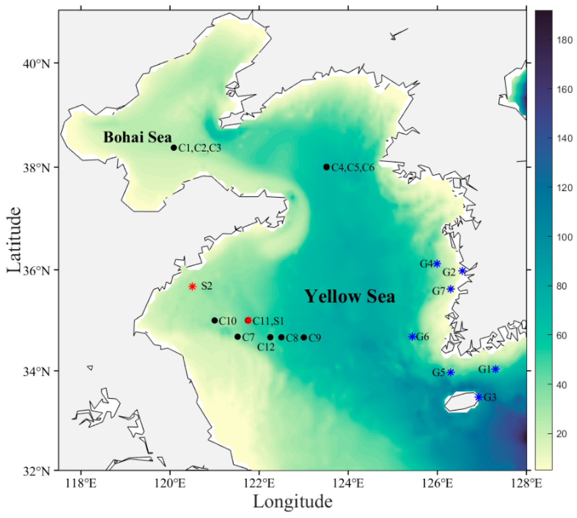
2.1. Data

The study area ranges zonally from 117.5°E to 131°E and meridionally from 24°N to 41°N, including the BYES, which is a broad continental shelf with significant tides and tidal currents (Figure 1). The harmonic constants of tidal constituents (M₂, S₂, K₁, O₁, N₂, K₂, P₁, and Q₁) are provided by X-TRACK tidal products. The long time series of SLA obtained from the Topex/Poseidon, Jason-1 and Jason-2 (T/P-Jason) missions were processed using X-TRACK software, with the processing of X-TRACK software, the outlines in altimetric corrections are more efficiently detected, the missing or rejected correction values are better reconstructed, and the correlation between near-shore altimetry sea level anomaly and tidal gauge records is substantially increased [30,31]. The tidal harmonic constants are derived by harmonic analysis of the improved SLA time series.

Tidal harmonic constants observed from 56 tide gauges (Figure 1, blue dots) are taken into account to validate the harmonic constants of SR. Due to data limitations, not all tide stations include harmonic constants of all eight tidal constituents. The harmonic constants of the four major constituents (M₂, S₂, K₁, O₁) are complete. There are 35 observed data for K₂ and P₁ constituents, and 24 and 22 observed data for N₂ and Q₁ constituents, respectively. Time series of SLA from two stations (S1 and S2, red asterisks in Figure 2) and seven tidal gauges (G1–G7, blue asterisks in Figure 2) are used to compare and validate the data. In addition, tidal current data are validated using twelve current velocity observations from eight sites located in the Bohai and Yellow Seas (C1–C12, black dots in Figure 2).

Five commonly used tidal model data are used to perform model validation. The Finite Element Solutions 2014 (FES2014) model (https://www.aviso.altimetry.fr/en/data/products/auxiliary-products/global-tide-fes/description-fes2014.html, accessed on 7 December 2017), a global tidal model based on the finite element method incorporates a wide range of data sources with a horizontal resolution of 1/16° [32]. TPXO9 (https://www.tpxo.net/global/tpxo9-atlas, accessed on 8 March 2018) is the latest version of the TPXO series of tidal models developed by Oregon State University, with a horizontal resolution of 1/6° at BYES [33]. EOT20 is the most recent version of an empirical ocean tide (EOT) model (https://doi.org/10.17882/79489) that used residual tide analysis from multi-mission satellite altimetry, with a horizontal resolution of 1/8° [34]. The National Astronomical Observatory 99b (NAO.99b) model (https://www.miz.nao.ac.jp/staffs/nao99, accessed on 25 June 2021) is a global ocean model with a spatial resolution of 1/2° that assimilated T/P altimeter data, the NAO.99Jb dataset with higher spatial resolution was also considered [35].

2.2. Model and Parameters

ROMS is a three-dimensional, free-surface numerical model that uses hydrostatic and Boussinesq assumptions and is primarily used in coastal areas [36]. It employs terrain-following vertical coordinates, which allow for improved vertical resolution in shallow water and regions with complex bathymetry [37]. The complete algorithm, numerical schemes, and physical parameterizations are described in detail in Shchepetkin and McWilliams [26,38].

ROMS is a three-dimensional, free-surface numerical model that uses hydrostatic and Boussinesq assumptions and is primarily used in coastal areas [36]. It employs terrain-following vertical coordinates, which allow for improved vertical resolution in shallow water and regions with complex bathymetry [37]. The model has a horizontal resolution of 1/12° and 10 vertical layers in the stretched terrain-following coordinates. In the model, temperature and salinity are set as spatially uniform in the entire domain. Atmospheric forcing, including wind, heat flux, and fresh water flux are also not included. In the open boundaries, only tidal forcing is considered.

In ROMS, there are two methods to impose tidal forcing for the model domain: (a) By specifying the time evolution of sea level at the open boundary and (b) by specifying the harmonic amplitudes and phases of the major tidal constituents. In this study, we forced the model using the second spectral method. ROMS uses a split-explicit time stepping scheme by advancing the three-dimensional (baroclinic) prognostic equations with larger time step and the depth-integrated (barotropic) prognostic equations with shorter time step [38]. The third-order upstream horizontal advection of 3D momentum and fourth-order centered vertical advection of momentum were used. The turbulence closure scheme is the generic length scale scheme. The complete algorithm, numerical schemes, and physical parameterizations are described in detail in Shchepetkin and McWilliams [26,38].

OBCs and BFCs are critical in the numerical simulation of marginal sea tides. In this study, these two spatially varying parameters were derived by processing T/P-Jason altimetry data.

OBCs are provided in the form of harmonic constants for the eight major tidal constituents at the open boundary (M₂, S₂, K₁, O₁, N₂, K₂, P₁, Q₁). However, the spatially discontinuous harmonic constants exported by X-TRACK cannot be directly applied as OBCs. To address this, the CPF method is used to directly fit the harmonic constants of satellite altimeter data. Chebyshev polynomials are orthogonal and are commonly used to smoothly describe continuous varying surfaces [16]. However, as a fitting method, the results of the CPF method are inevitably affected by the low accuracy and limited quantity of observations near the coast, resulting in deviations from actual conditions. This is also reflected in the cotidal charts drawn by Wang et al. [19]. As the open boundary is adjacent to the open ocean, the CPF method can be effectively utilized [16]. Therefore, the harmonic constants derived by altimeter data are fitted using the CPF method to obtain OBCs with the required resolution for spatial continuity.

BFCs cannot be directly calculated through altimeter observations and are generally derived through empirical functions [39,40]. Data assimilation methods can quantitatively estimate model parameters that vary spatially or temporally by minimizing the difference between simulation and observation [41]. The adjoint method, which has been widely used in the oceanic and atmospheric models is a powerful tool for estimating parameters [29]. However, using the adjoint assimilation method to numerically simulate multiple tidal constituents with high horizontal resolution over a large area requires a significant amount of computational resources. This is difficult to achieve in some applications. The adjoint method has been widely used to assimilate altimeter data to estimate spatially varying BFCs and has achieved excellent results. Therefore, this study uses the adjoint assimilation method to obtain BFCs and achieve improved simulation results. BFCs are estimated by assimilating T/P-Jason altimeter data using the adjoint method, details of the method can be found in Lu and Zhang [27].

The hindcast run started at 0:00 on 1 October 2019, with a time step of 2 min, and the total duration of the simulation is 450 days. Cao et al. [42] suggest that for the simultaneous simulation of multiple tidal constituents, the appropriate time span of sea level anomaly (SLA) series for harmonic analysis is approximately 1 year. As the model requires a stable process, the initial 90-day-long data of the simulation are not available.

Following the numerical simulation, time series data of SLA and tidal currents that span a length of 562.5 days are obtained, the harmonic analysis is performed on the data from the last 360 days to obtain the harmonic constants of the eight major tidal constituents. In this process, the CPF method is used to compare the altimeter data with the model simulation results and adjust the model parameters based on the comparison results to further optimize the SR.

The harmonic constants of the altimeter and the coastal tide gauges are respectively used to verify data from different models. The root-mean-square (RMS) differences [7], the absolute mean errors (MAEs) of amplitude and phase are calculated as:

$$\begin{gathered} \mathrm{R}\mathrm{M}\mathrm{S}={\left(\frac{1}{2N}{\sum }_{i=1}^N{\left[{\overline{A}}_i\mathit{cos}\left({\overline{P}}_i\right){-A}_i\mathit{cos}\left(P_i\right)\right]}^2+{\left[{{\overline{A}}_i\mathit{sin}\left({\widehat{P}}_i\right)-A}_i\mathit{sin}\left({\overline{P}}_i\right)\right]}^2\right)}^{1/2} \\ ∆A=\frac{1}{N}{\sum }_{i=1}^N\left|{\overline{A}}_i{-A}_i\right| ,\hspace{1em}∆P=\frac{1}{N}{\sum }_{i=1}^N\left|{\overline{P}}_i{-P}_i\right| \end{gathered}$$

where $\overline{A}$ and $\overline{P}$ are the observed amplitudes and phases, $A$ and $P$ are the simulated amplitudes and phases, $∆A$ is the MAE of amplitude, and $∆P$ is the MAE of phase.

3. Results

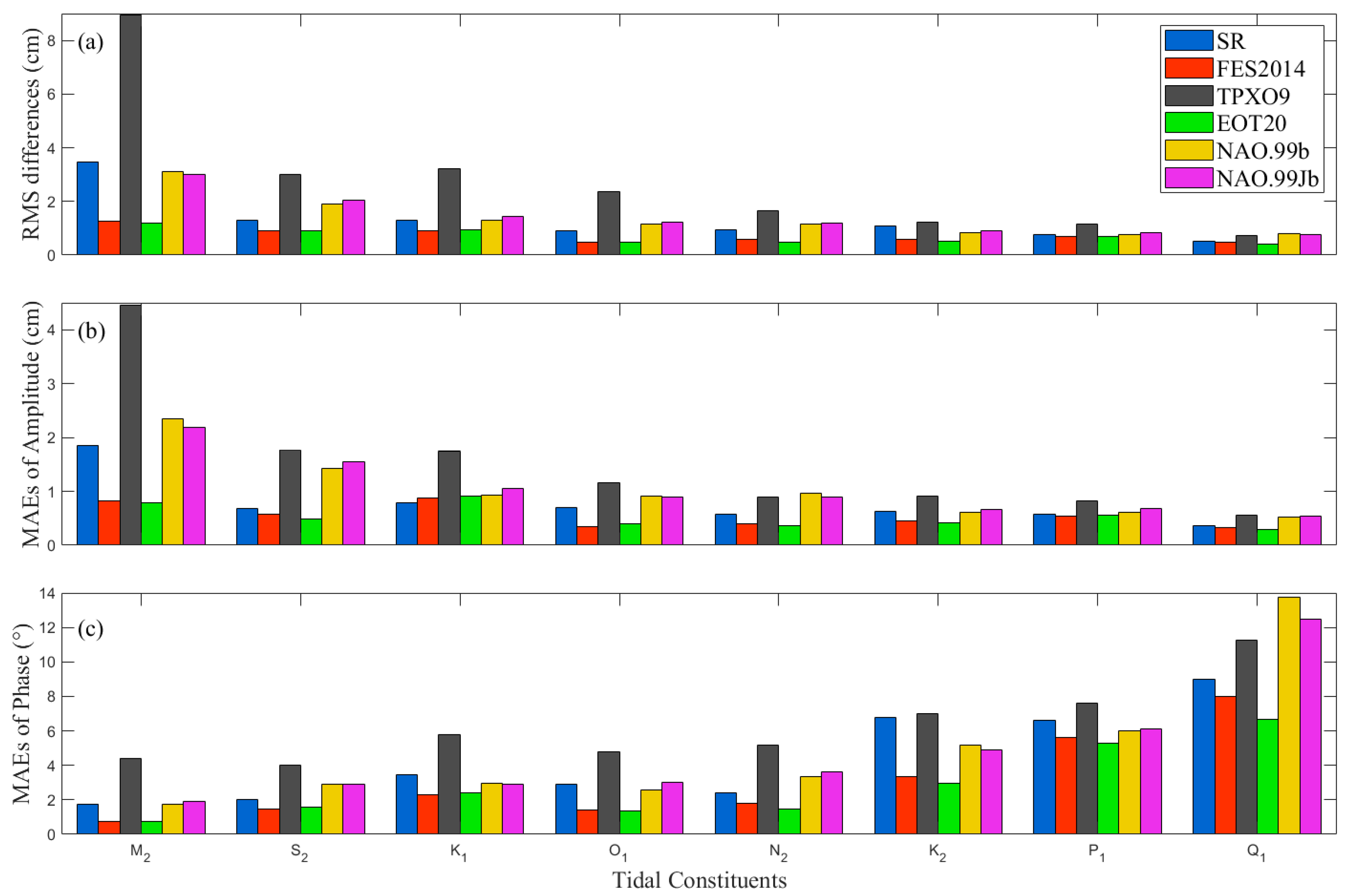
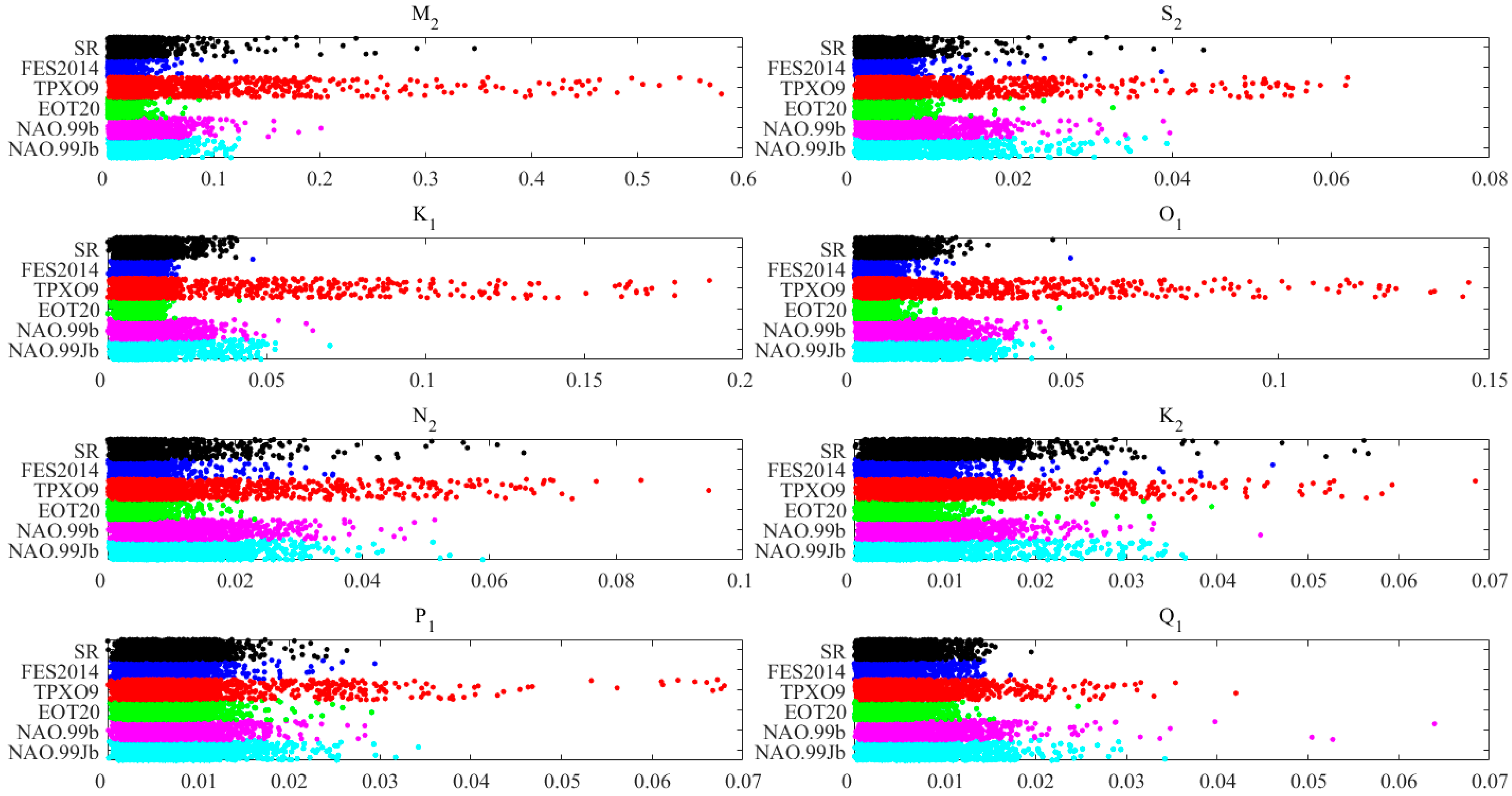
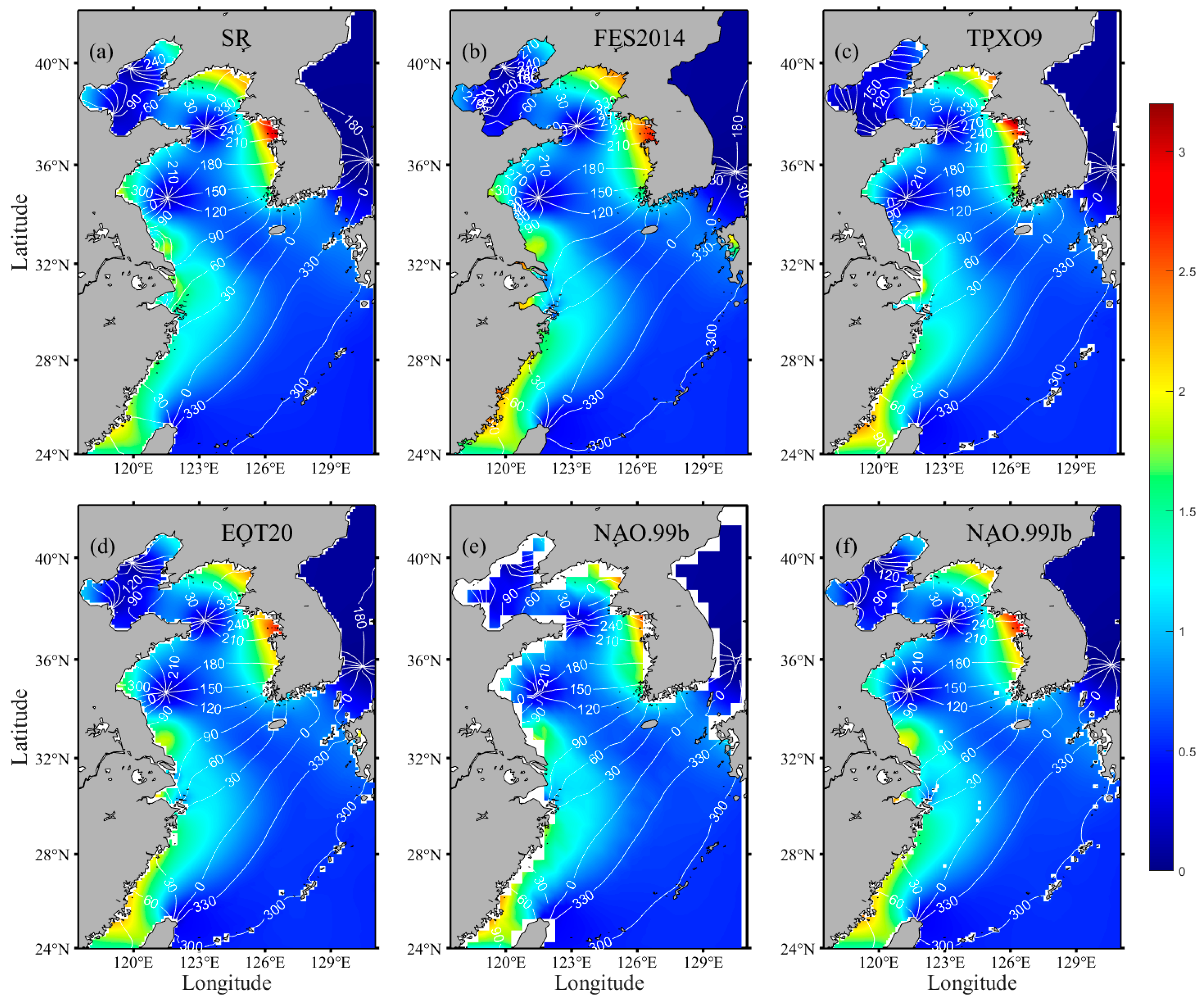
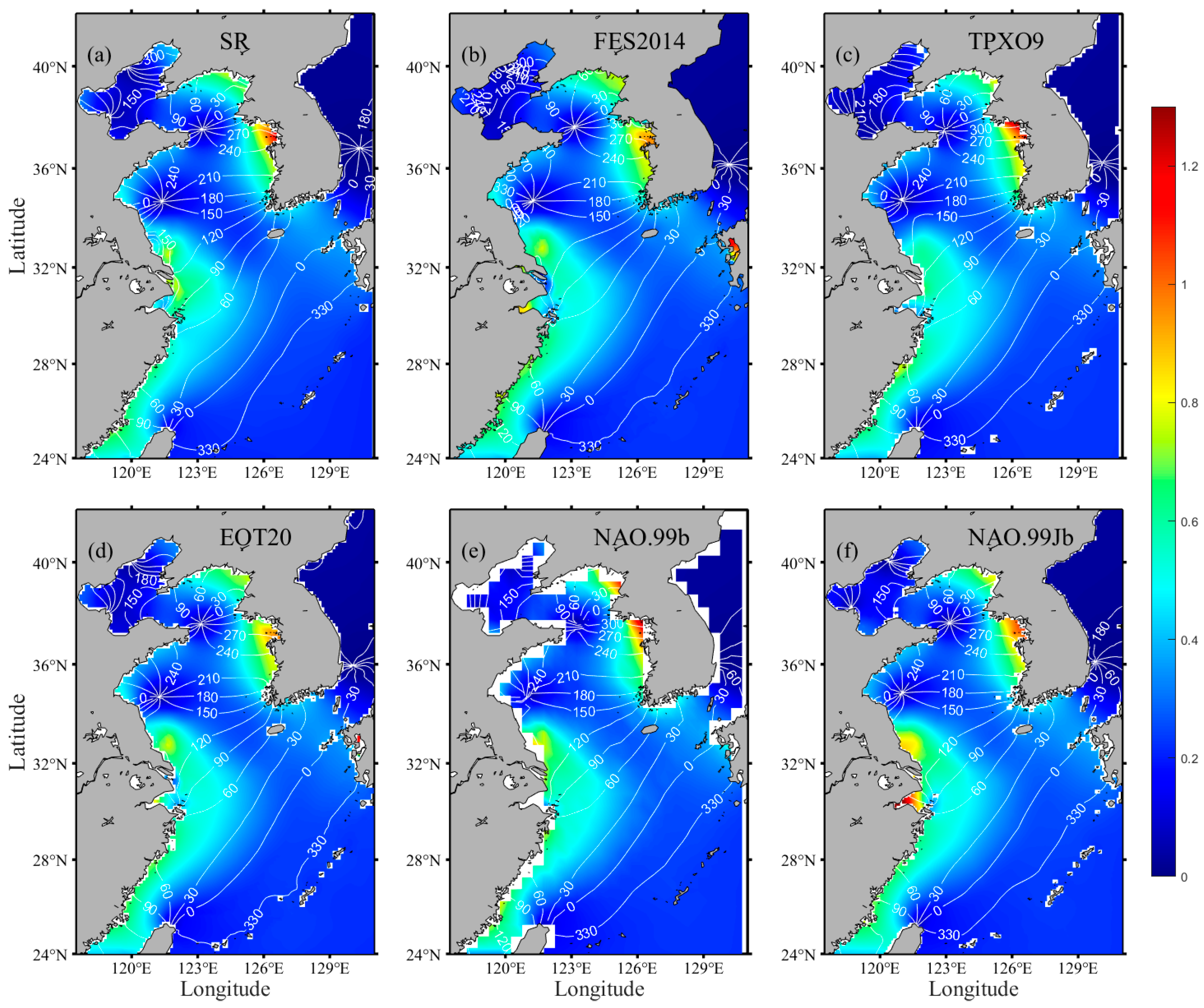
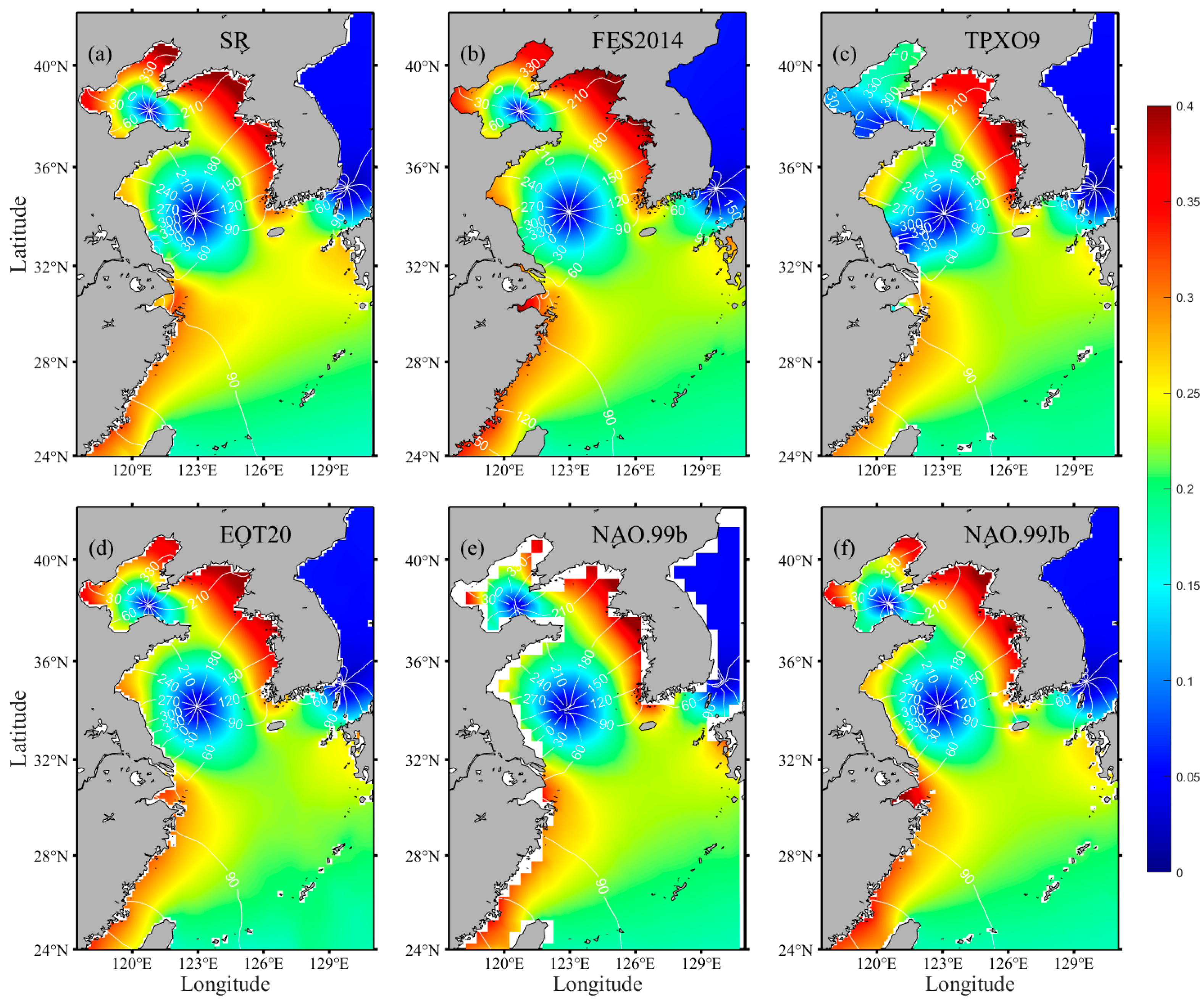
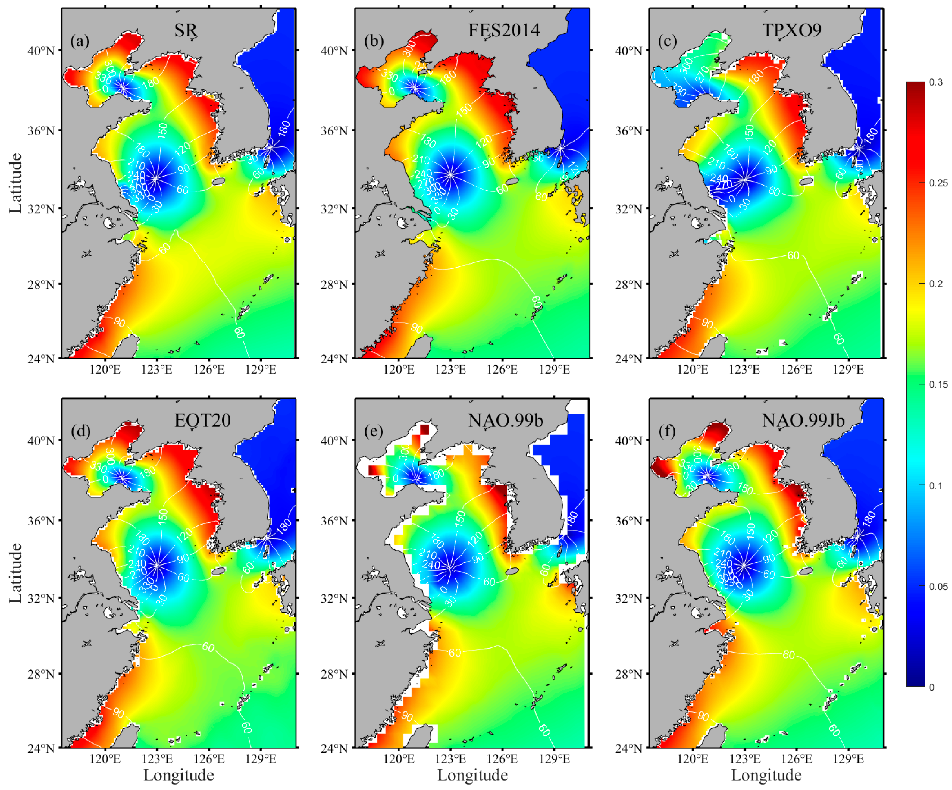
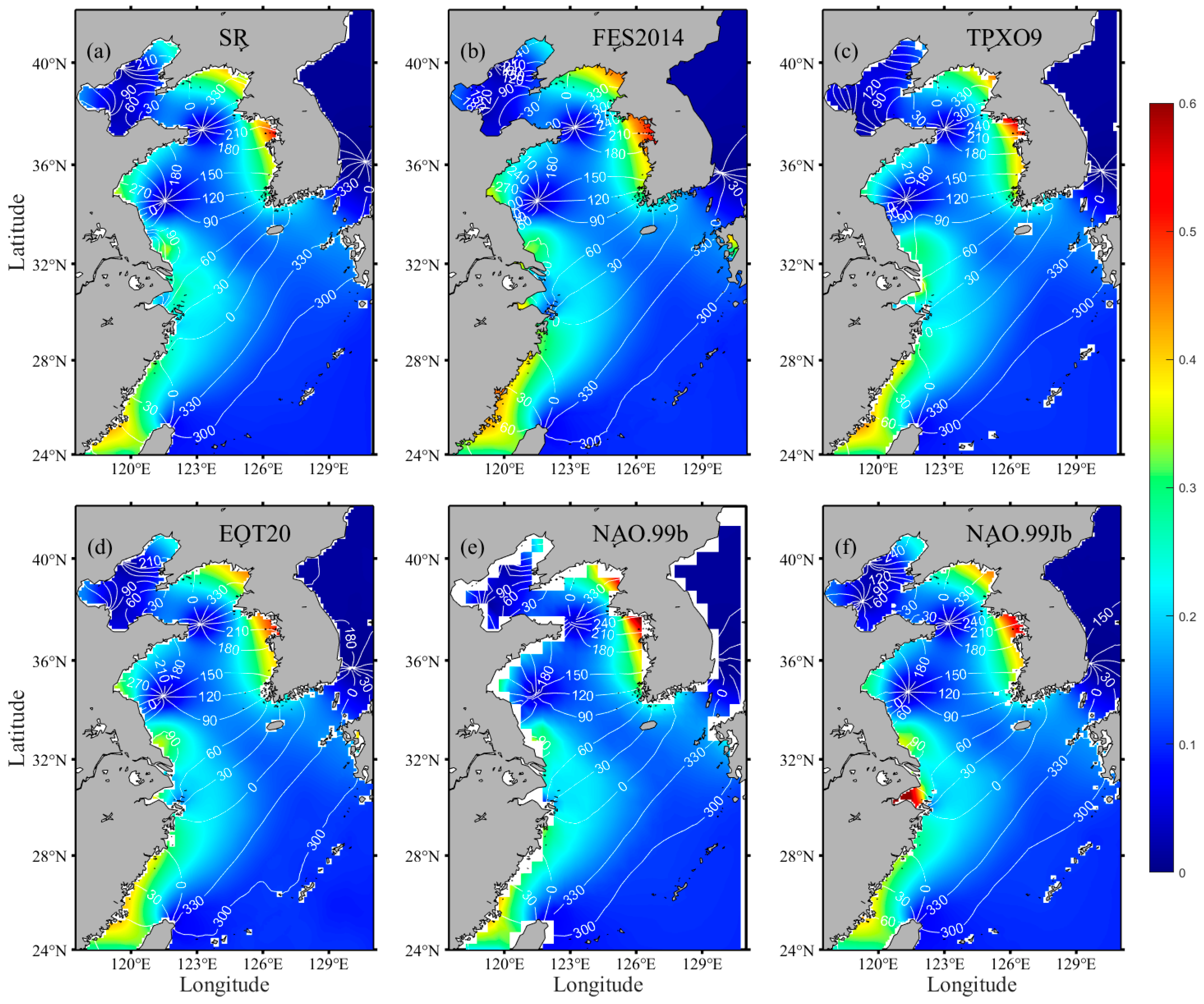
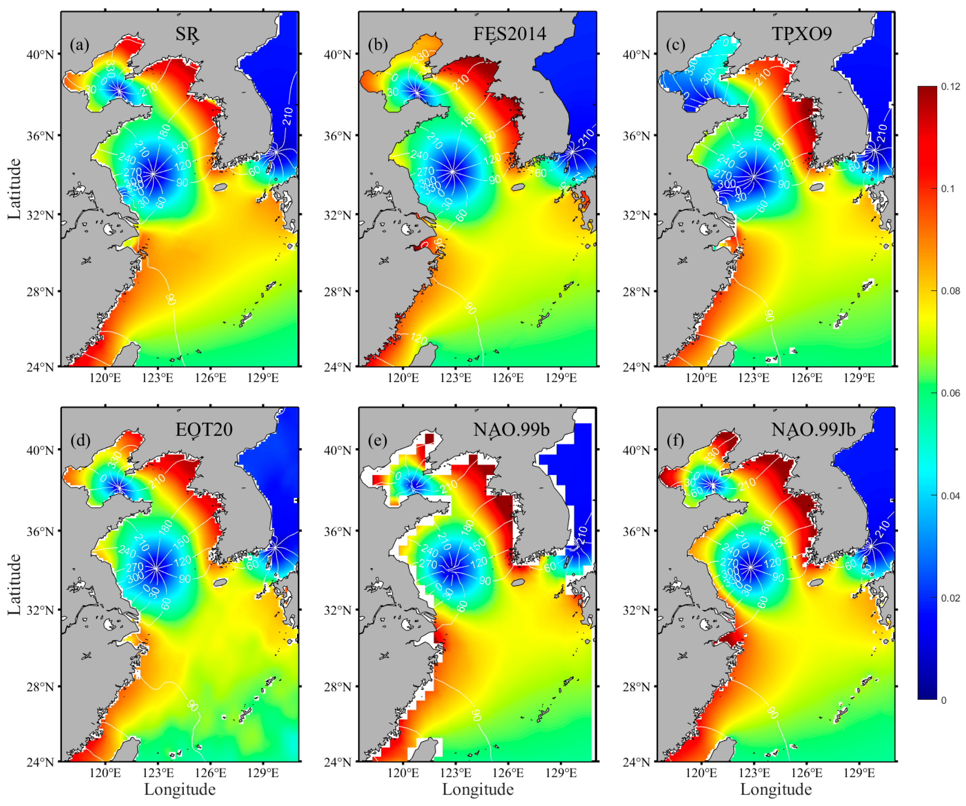
3.1. Harmonic Constants Validation with T/P-Jason Data

Using T/P-Jason data to validate SR, the RMS differences and MAEs of harmonic constants are calculated. The RMS differences for the eight major constituents are 3.48 cm, 1.29 cm, 1.30 cm, 0.89 cm, 0.94 cm, 1.09 cm, 0.77 cm, and 0.52 cm (M₂, S₂, K₁, O₁, N₂, K₂, P₁, and Q₁). Additionally, results from five ocean tide models are included for comparison. The RMS differences, MAEs of the amplitude and phase are shown in

Table 1. RMS differences and MAEs of harmonic constants derived from SR and five ocean tidal models compared to T/P-Jason data.

RMS (cm)	M2	S2	K1	O1	N2	K2	P1	Q1
SR	3.48	1.29	1.30	0.89	0.94	1.09	0.77	0.52
FES2014	1.26	0.92	0.92	0.47	0.57	0.60	0.68	0.48
TPXO9	8.94	3.00	3.22	2.35	1.64	1.24	1.15	0.74
EOT20	1.20	0.91	0.96	0.48	0.47	0.52	0.69	0.42
NAO.99b	3.10	1.91	1.31	1.17	1.17	0.85	0.78	0.80
NAO.99Jb	3.01	2.04	1.43	1.22	1.20	0.89	0.85	0.77
$∆\mathit{A}$ (cm)	M2	S2	K1	O1	N2	K2	P1	Q1
SR	1.86	0.68	0.78	0.70	0.58	0.63	0.58	0.37
FES2014	0.82	0.57	0.87	0.34	0.39	0.45	0.54	0.33
TPXO9	4.46	1.77	1.75	1.16	0.89	0.91	0.82	0.56
EOT20	0.79	0.49	0.92	0.39	0.36	0.41	0.55	0.30
NAO.99b	2.35	1.43	0.93	0.92	0.96	0.62	0.61	0.53
NAO.99Jb	2.18	1.55	1.06	0.90	0.89	0.66	0.68	0.54
$∆\mathit{P}$ (°)	M2	S2	K1	O1	N2	K2	P1	Q1
SR	1.76	2.01	3.45	2.88	2.43	6.77	6.60	9.00
FES2014	0.73	1.48	2.28	1.40	1.80	3.36	5.62	7.98
TPXO9	4.42	4.00	5.79	4.81	5.16	7.01	7.59	11.25
EOT20	0.75	1.60	2.42	1.35	1.47	2.97	5.29	6.68
NAO.99b	1.72	2.89	2.97	2.59	3.36	5.19	6.02	13.76
NAO.99Jb	1.89	2.89	2.88	3.01	3.61	4.91	6.13	12.48

. The average amplitudes of the altimeter observations of M₂, S₂, K₁, and O₁ constituents in this area are 77.49 cm, 30.44 cm, 21.12 cm, and 16.27 cm, respectively. The simulated difference ratios of the amplitudes (ratio of MAEs of amplitude to average amplitude) of these four constituents of SR are all less than 5%. The average amplitudes of the remaining four constituents are less than 15 cm, and the simulated difference ratio was in the range of 4–12%. Numerically, SR simulates the eight major tidal constituents of BYES well and has good performance.

The histogram of the differences between each data and satellite observation provides a more visual comparison of the effectiveness of each model data (Figure 3). For all tidal constituents, the RMS differences between FES2014 and EOT20 compared to the altimeter data are close and the smallest. FES2014 and the altimeter data agree well, which may be attributed to the assimilation method of FES2014 and its assimilation of more observations, including T/P-Jason altimeter data [7,43]. EOT20 data also incorporate a large amount of observational and model data, and is based on FES2014 as a reference, resulting in the two having very similar performances [34]. NAO.99b and NAO.99Jb (NAO) perform slightly worse, while TPXO9 has the largest RMS difference with altimeter data among the five models. In the altimeter validation, for the M₂ and K₂ constituents, SR performs close to NAO and better than TPXO9. For the S₂, K₁, O₁, and N₂ constituents, the RMS differences for SR are smaller than TPXO9 and NAO.99b and slightly larger than FES2014 and EOT20. For the P1 and Q1 constituents, the RMS differences for SR were smaller than TPXO9 and NAO and slightly larger than FES2014 and EOT20.

After processing with X-TRACK software, there are a total of 1788 observation data from T/P-Jason altimeters in BYES. The RMS differences for each observation are calculated and counted as in Figure 4. More evident than in Table 1, the performance of SR in semidiurnal tide is close to NAO and better than TPXO9. However, there are some data with large RMS differences, which also exist in other models. The performance of SR in the diurnal constituents is relatively good, similar to that of FES2014 and EOT20, with few data points showing a significant RMS difference.

The crossover points are the intersection of ascending and descending satellite altimeter tracks. At the crossover points, the satellite observes twice in a single period, with more data than other observation points and a higher signal-to-noise ratio [17]. As a result, tidal constituents information obtained at crossover points are more reliable. The altimeter data at crossover points are extracted for harmonic analysis, the SR and other model data are validated and compared (

Table 2. RMS differences between different datasets and T/P-Jason data at crossover points.

	M2	S2	K1	O1	N2	K2	P1	Q1
SR	2.66	0.99	1.13	0.84	0.79	1.13	0.76	0.33
FES2014	1.04	0.80	0.41	0.38	0.42	0.65	0.52	0.26
TPXO9	3.62	1.63	1.13	1.10	0.75	1.39	0.83	0.60
EOT20	1.33	0.90	0.51	0.56	0.38	0.66	0.64	0.31
NAO.99b	1.65	1.32	0.72	1.13	1.02	1.01	0.64	0.56
NAO.99Jb	2.23	1.53	0.59	1.31	0.96	0.92	0.59	0.61

). The RMS differences for all constituents of SR, except for the K₂ constituent, decreased compared to Table 1. Apart from EOT20, data in other modes also exhibit the same variations. This variation may be due to the fact that most crossover points are located in deeper waters where amplitudes of tidal constituents are small and errors are relatively small. In addition, there is a larger amount of data near the crossover points, which is conducive to data assimilation and correction. According to Table 2, SR also have good performance in crossover validation.

3.2. Harmonic Constants Validation with Tidal Gauges Data

The data from tide gauges in the BYES are also used to validate the performance of SR, and the corresponding RMS differences and MAEs are calculated. The RMS differences for M₂, S₂, K₁, O₁, N₂, K₂, P₁, and Q₁ constituents are 9.22 cm, 5.57 cm, 2.73 cm, 3.76 cm, 1.96 cm, 1.57 cm, 0.90 cm, and 0.82 cm, respectively. The results of the five models are also used for comparison (

Table 3. RMS differences and MAEs of harmonic constants derived from SR and five ocean tidal models compared to tide gauges data.

RMS (cm)	M2	S2	K1	O1	N2	K2	P1	Q1
SR	9.22	5.57	2.73	3.76	1.96	1.57	0.90	0.82
FES2014	7.55	4.54	2.74	3.72	1.74	1.32	0.89	0.83
TPXO9	9.63	5.52	3.53	4.40	2.45	1.18	0.98	1.03
EOT20	7.21	4.33	2.87	4.07	1.18	1.01	0.82	0.86
NAO.99b	14.59	6.90	3.40	4.29	2.60	1.30	0.91	0.87
NAO.99Jb	7.34	4.48	3.72	4.79	1.89	1.52	1.10	1.07
$∆\mathit{A}$ (cm)	M2	S2	K1	O1	N2	K2	P1	Q1
SR	5.51	2.91	1.63	1.29	1.08	0.97	0.57	0.45
FES2014	4.34	2.87	1.74	1.27	1.17	0.81	0.57	0.43
TPXO9	5.48	2.87	2.16	1.47	1.22	0.69	0.72	0.70
EOT20	4.05	2.51	1.72	1.16	0.76	0.55	0.66	0.51
NAO.99b	7.74	4.09	2.39	1.88	1.28	0.67	0.69	0.58
NAO.99Jb	3.95	2.89	2.37	1.72	1.08	0.77	0.82	0.79
$∆\mathit{P}$ (°)	M2	S2	K1	O1	N2	K2	P1	Q1
SR	6.26	8.61	3.79	5.72	8.61	10.03	5.10	9.72
FES2014	4.85	6.76	3.74	5.34	4.15	8.18	4.58	10.57
TPXO9	5.18	7.78	4.75	8.02	6.67	8.31	4.51	8.11
EOT20	4.79	6.94	3.70	6.16	4.98	8.74	3.54	9.73
NAO.99b	7.11	8.84	3.99	5.80	9.16	9.61	4.23	9.49
NAO.99Jb	5.57	7.75	5.03	7.05	7.13	12.16	5.09	9.68

). Compared to Section 3.1, SR and each model data all show a decrease in performance at the coastal tide gauges, with the most significant deterioration in the M₂ and S₂ constituents. Although FES2014 and EOT20 still perform well on the semidiurnal constituents, the gap between SR and the two models is reduced compared to the altimeter data verification. In terms of diurnal constituents, the effects of the K₁, O₁, and Q₁ constituents of SR are the best. This suggests that SR is effective in coastal areas and has performance that surpasses several widely recognized model data in some partial tidal constituents. It is worth noting that NAO.99Jb performs significantly better than NAO.99b in the M₂ and S₂ constituents in the validation with the tide gauge stations, which somehow suggests that the improved spatial resolution is helpful in optimizing the numerical simulation of coastal tides.

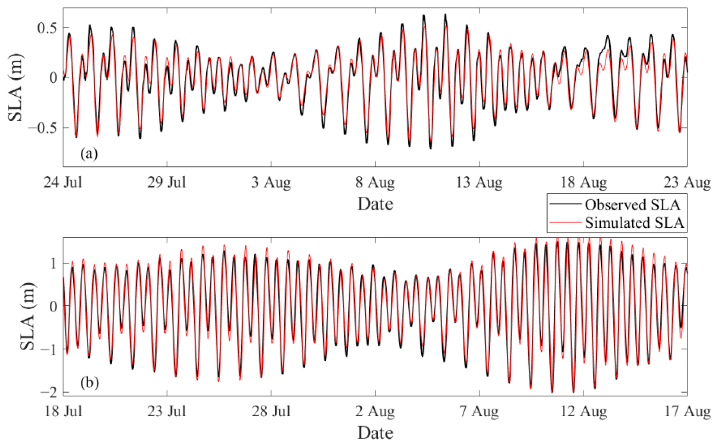
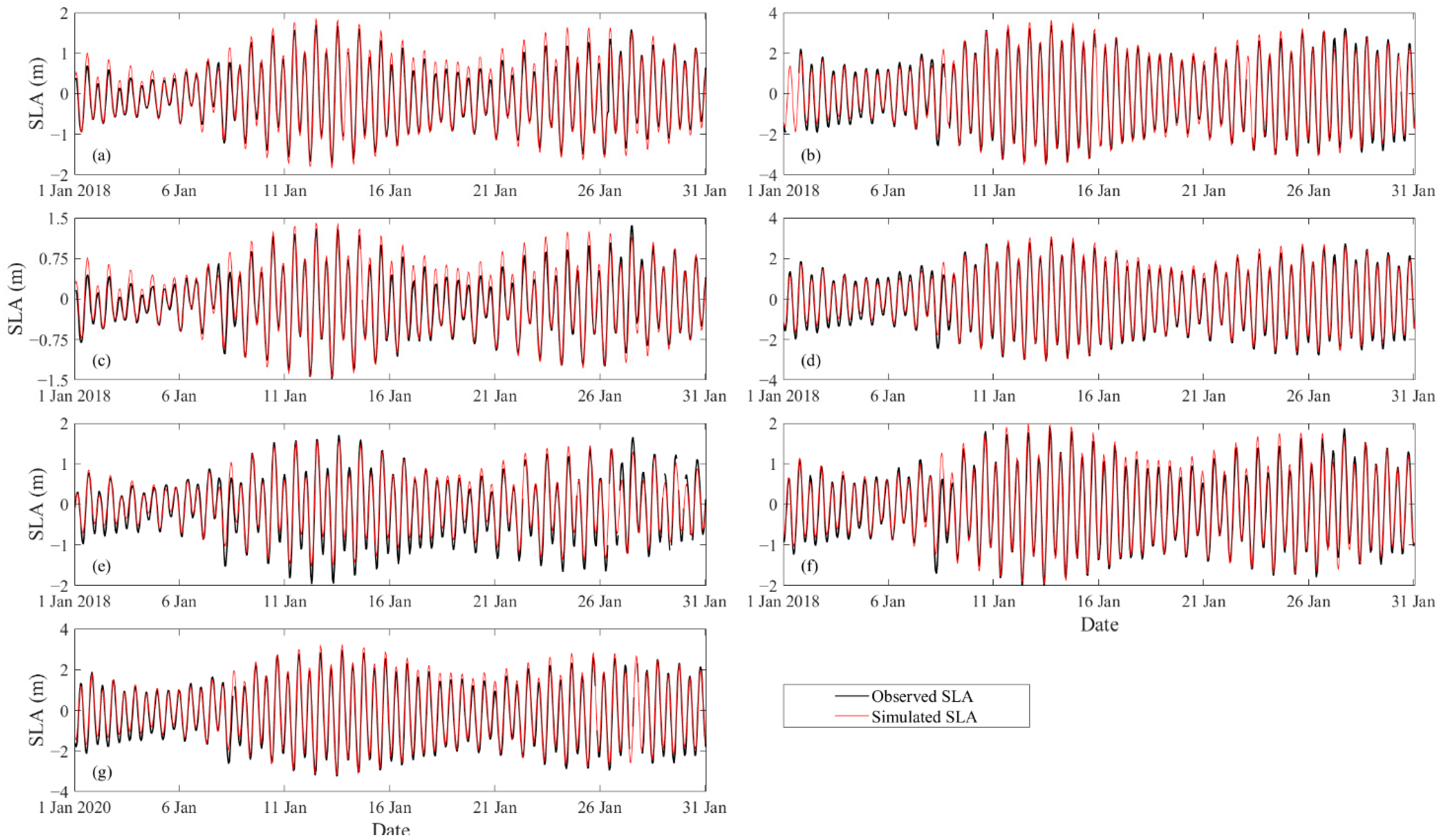
3.3. Water Elevation Validation

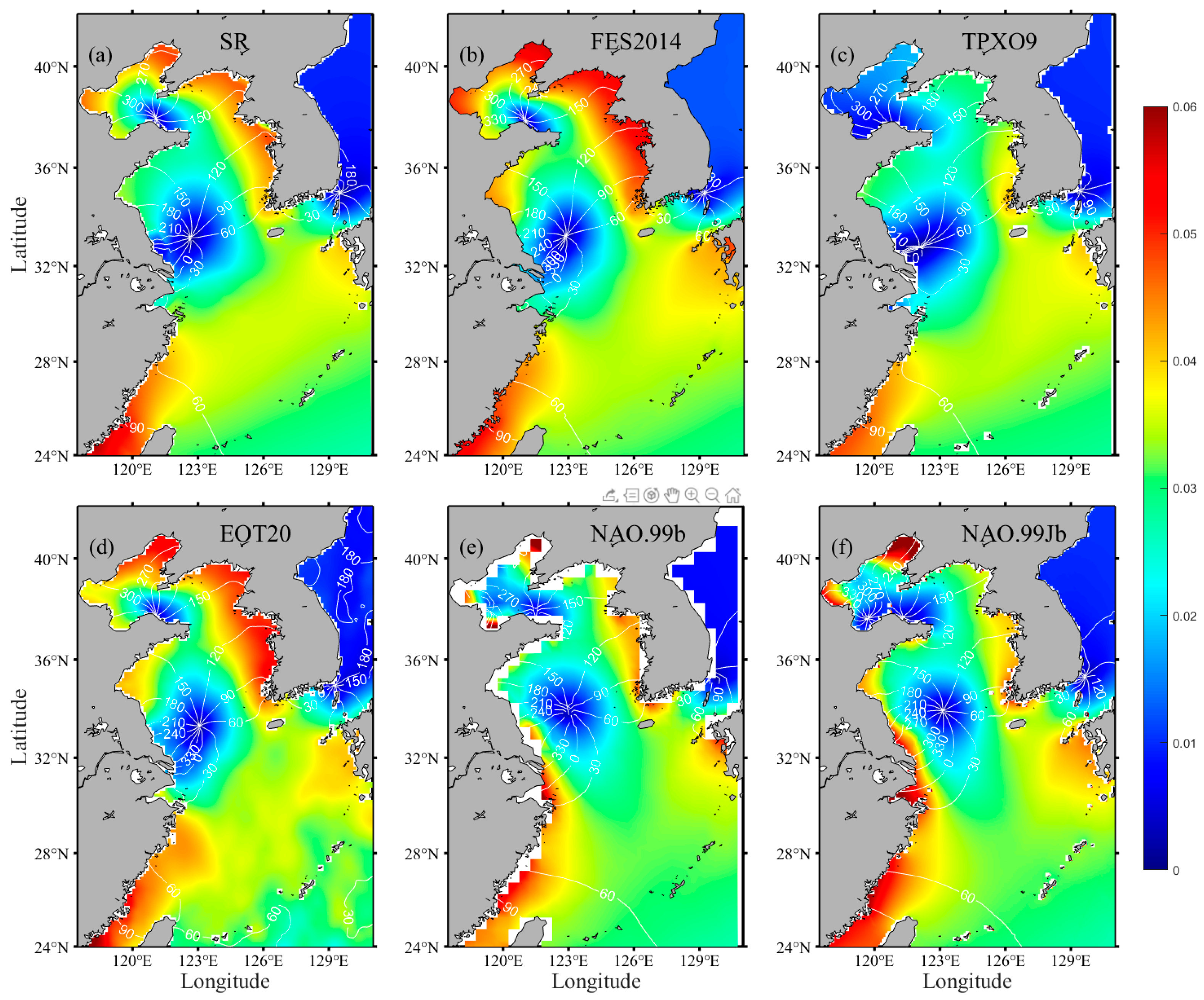
Nine SLA time series from two stations located in the Yellow Sea (red asterisks in Figure 2) and seven gauges (blue asterisks in Figure 2) are used to verify the accuracy of the data. The observation interval for both time series from S1 and S2 is 30 min, and the total time span is greater than 30 days for both time series. Due to the poor accuracy of the initial period of observations, only the last 30 days of data (Figure 5) were selected for processing and analysis for comparison purposes. The start time for the data at the first station (S1) is 6:30 on 24 July 2007, while the start time for the data at the second station (S2) is 12:30 on 18 July 2007. The observation interval for time series from G1–G7 is 1 h, the total time span from G1–G6 is 3 years, and the total time span for G7 is 1 year. The start time for data from G1–G6 is 0:00 on 1 January 2018 and the start time for data for G7 is 0:00 on 1 January 2020. Due to the large amount of original data, only the results of the first month of each time series are selected for display (Figure 6).

The water depth at the location of station S1 is deeper than that of station S2, and the SLA variation amplitude at S1 is smaller, ranging from −0.8 m to 0.7 m, while the SLA range at S2 station is from −2 m to 1.6 m. The tidal type of both stations is an irregular semidiurnal tide; however, the inequality of tides at S1 station is more prominent. The SLA difference of some adjacent high and low tides is very small. G1–G7 are located in the eastern side of the Yellow Sea, the tidal types are also an irregular semidiurnal tide, and the SLA variation amplitudes are greater than those of S1 and S2.

The simulated SLA series obtained through SR show good consistency with the observations. At the temporal resolution of the observational data, the timing of simulated and observed high and low tides in SLA is the same. The MAEs of simulated and observed SLA at S1 and S2 are 4.84 cm and 11.59 cm, respectively. The simulated SLA has a relatively smaller amplitude for S1 compared to the observed SLA, manifested as relatively higher low-tide levels and relatively lower high-tide levels. The opposite is true in S2, where the amplitude of the simulated SLA is higher than observed SLA. The SLA comparison of G5 shows similar characteristics to S1, while the SLA comparison of G1 and G3 shows similar characteristics to S2. The rest of the simulation results also show good agreement with the tide gauge data. However, the magnitude of the error is within a reasonable range compared to the observations.

Calculations of MAE for simulated and observed SLA are obtained by using the harmonic constants of SR to calculate the SLA time series (Figure 5 and Figure 6), respectively. Additionally, SLA time series and MAE are derived for five models using the same method (

Table 4. MAE (unit: cm) of SLA derived from SR and five ocean tidal models compared to SLA from two stations in the Yellow Sea.

	SR	FES2014	TPXO9	EOT20	NAO.99b	NAO.99Jb
S1	4.84	4.29	5.75	4.19	38.34	4.29
S2	11.59	10.07	10.00	10.16	96.57	10.07
G1	14.64	12.02	12.61	12.04	15.24	12.29
G2	22.05	22.31	22.80	21.93		26.65
G3	14.55	13.77			16.74	14.74
G4	17.58	16.61	17.32	16.64	16.66	16.32
G5	15.05	14.06	14.33	14.11	16.48	15.26
G6	16.26	14.37	18.62	14.34	13.60
G7	20.64	18.33	24.93	18.18

).

In the SLA validation of G1–G7, the evaluation results of SR and model data are very close, and the data performance varies in different observations. In the SLA validation of S1 and S2, the evaluation results of NAO.99b show a large error, which may be affected by its lower horizontal resolution. Combined with Figure 5 and Figure 6 and Table 4, SR also has excellent and stable performance in the calculation of SLA and can be well applied to the forecasting and research of water level.

3.4. Cotidal Charts

Based on the harmonic constants from SR and five models, cotidal charts for eight major constituents are given, respectively (Figure 7, Figure 8, Figure 9, Figure 10, Figure 11, Figure 12, Figure 13 and Figure 14). Compared to the cotidal charts obtained from the five models, the SR also adequately reflects the spatial characteristics of the eight major tidal constituents in BYES. Tidal waves of different constituents are transmitted from the Pacific Ocean to BYES and form different numbers of counterclockwise rotating tidal systems under the action of topography and Coriolis force. The tidal semidiurnal constituents represented by the M₂ constituent have four rotating tidal systems and four amphidromic points in the Bohai Sea and Yellow Sea, while the tidal diurnal constituents represented by the K₁ constituent have one amphidromic point in the Bohai Sea and one in the Yellow Sea. Under the influence of friction, the amphidromic points are located to the left of the central axis of the sea area, which also causes the amplitude on the east coast to be slightly larger than that on the west coast [44]. At the same time, under the influence of topography, the amplitude at the top of the bay is larger than the other areas, such as in Gyeonggi Bay on the west side of Korea [45], which is more evident in the semidiurnal constituents.

The SR model’s spatial resolution is only surpassed by that of FES2014. It can accurately display the location of amphidromic points with good continuity. NAO99b has the lowest spatial resolution among the models, resulting in some discontinuity in its spatial representation, especially near amphidromic points. Compared to the other model data, the TPXO9 model has smaller amplitudes and different co-phase lines in the Bohai Sea and southwest side of the Yellow Sea. This is especially evident for the diurnal tidal constituents (Figure 8c, Figure 9c, Figure 12c, and Figure 13c). The cotidal charts of SR, EOT20, and FES2014 have similar characteristics. However, it should be noted that the K₂ (Figure 11d) and Q₁ (Figure 13d) cotidal charts of EOT20 display some disorder in the region of the first island chain and the Japan Sea.

According to the cotidal charts, the SR effectively captures the characteristics of the eight major tidal constituents in BYES. This provides an effective reference for studying the long-term changes in sea level in BYES and its internal regions and for drawing the chart datum and other work.

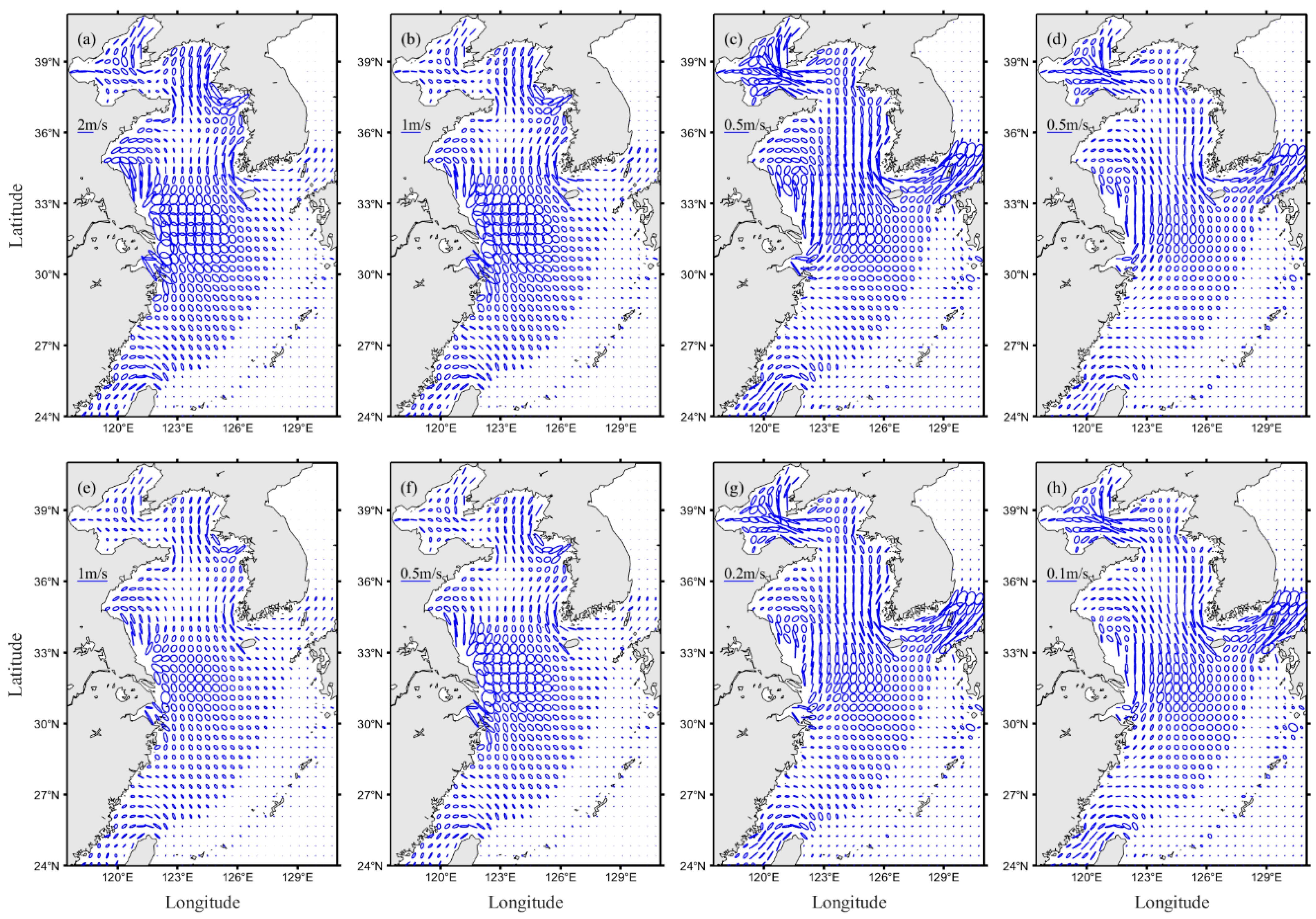
3.5. Tidal Current Validation

By conducting depth-averaging and harmonic analysis on the current velocity data of SR, the two-dimensional tidal harmonic constants for eight major constituents are obtained. The tidal current data are validated using twelve current velocity observations from eight sites located in the Bohai and Yellow Seas (Figure 15). The observation time of these current velocity data is between July 2006 and October 2007, with observation durations ranging from 30 to 100 days and an observation interval of 1 h.

To eliminate the influence of background flow and other non-tidal factors in the observed current velocity data, harmonic analysis is conducted on 12 sets of current velocity time series. Using harmonic constants, the zonal and meridional velocities (u and v) are calculated for the 30 days prior to each observation, after which the tidal current data of SR are validated (

Table 5. The MAE of the zonal velocity, meridional velocity between SR and the processed observation data, and the average velocity magnitude of the processed observation data (unit: cm/s).

	u	v	Max
1	14.11	5.53	76.28
2	13.80	4.21	68.67
3	13.38	4.59	70.75
4	10.92	10.06	77.00
5	4.65	8.27	88.09
6	3.97	9.73	86.10
7	8.75	5.36	69.17
8	3.99	6.18	66.53
9	3.58	6.33	55.45
10	9.03	6.46	74.07
11	8.94	6.48	49.87
12	4.56	7.05	54.62

), where Max is the maximum magnitude of the velocity vector. The differences between SR and observation data are all below 15 cm/s. The water depth of the stations (C1–C6) in the Bohai Sea and the North Yellow Sea is relatively shallow, the velocity is relatively high, and the MAEs are relatively large. The velocity of the stations in the Yellow Sea is relatively small, and the MAEs are all less than 10 cm/s.

The tidal current ellipses of the eight major tidal constituents are drawn based on the SR tidal data (Figure 15). It can be seen that the semidiurnal tidal currents are relatively strong in the Yangtze River Delta and on the west side of the Korean Peninsula, which is consistent with the high amplitude area of the cotidal chart. The diurnal tidal currents are relatively strong in the Bohai Sea and the Korea Strait. Wang et al. [29] and Guo and Yanagi [46] conducted simulations and studies on the M₂, S₂, K₁, and O₁ tidal constituents of BYES, and the tidal current ellipses of SR (Figure 15) are similar to their tidal ellipses. This also indicates that SR well reflects the characteristics of the tidal currents in BYES.

It can be noticed that the difference between the tidal simulation and observation is larger compared to the SLA, which may be mainly caused by the lack of observation. On the one hand, SLA observation technology is well developed, with wide spatial and temporal distribution and small errors. However, acquiring ocean current observation data is difficult and there is strong spatiotemporal variability. In the numerical simulation process, more consideration will be given to the SLA observational data, which may result in significant differences between the simulated current values and the observed data. On the other hand, tidal signals are relatively easy to distinguish in SLA. However, there are more factors influencing ocean currents, especially when the actual ocean is in a state of baroclinic, it can be difficult to accurately distinguish the barotropic tidal current signal in velocity observations.

4. Conclusions

This paper employs ROMS to conduct numerical simulations of the eight major tidal constituents (M₂, S₂, K₁, O₁, N₂, K₂, P₁, and Q₁) in the BYES. The two main parameters of the model, the OBCs and BFCs, are obtained from T/P-Jason altimeter data provided by X-TRACK. The OBCs are obtained by processing harmonic constants derived from altimeter data using the CPF method. The BFCs are obtained by assimilating T/P-Jason data using the adjoint method. Tidal harmonic constants and tidal current data for the study area are then obtained through harmonic analysis. The SR are validated using various data sources, including satellite altimeter data, tidal gauges observation data, and current meters.

The tidal harmonic constants are validated using satellite altimeter and tide gauges data, and data from five tidal models are also used for comparison. The RMS differences between the simulation results and the altimeter are 3.48 cm, 1.29 cm, 1.30 cm, 0.89 cm, 0.94 cm, 1.09 cm, 0.77 cm, and 0.52 cm (M₂, S₂, K₁, O₁, N₂, K₂, P₁, and Q₁), respectively. Based on the results of the model comparison, the harmonic constants of SR exhibit good agreement with the altimeter data, especially for the diurnal tidal constituents. The RMS differences between the SR and the tide gauges data are 9.22 cm, 5.57 cm, 2.73 cm, 3.76 cm, 1.96 cm, 1.57 cm, 0.90 cm, and 0.82 cm, respectively. The difference between all tidal models and tide gauge data has increased compared to their difference with the altimeter. However, the error of SR has not increased significantly, and SR still maintains a relatively good performance. In the SLA time series validation, the SR and observed SLA have good consistency, indicating that SR can be well used for water level calculation and forecasting. The tidal charts of SR have a high horizontal resolution (second only to FES2014) and reflect the characteristics of the eight major tidal constituents of BYES well. Verifying of the tidal data of SR through 12 ocean current meter data and tidal current ellipses of eight major tidal constituents are drawn. The comparison results show that SR have a high degree of consistency with the actual observed data, verifying the effectiveness and reliability of the data and method.

As the BYES is one of the most complex regions for tides and tidal currents, research on BYES tides is important and necessary. After comparison and verification, the product of this work can provide support for observation instrument calibration in ocean observation, depth reference calculation in ocean engineering, and other related research on BYES tides and tidal currents. It is of great significance for deepening the understanding of the tidal characteristics of the BYCS, optimizing marine forecasts, and protecting the marine environment. In subsequent works, we will also further study the tides of BYES, including research on three-dimensional tidal currents, shallow water tidal constituents, and higher resolution simulations.

References

1. Munk, W.; Wunsch, C. Abyssal recipes II: Energetics of tidal and wind mixing. Deep. Res. Part I Oceanogr. Res. Pap. 1998, 45, 1977–2010. [Google Scholar] [CrossRef]
2. Vic, C.; Naveira Garabato, A.C.; Green, J.A.M.; Waterhouse, A.F.; Zhao, Z.; Melet, A.; de Lavergne, C.; Buijsman, M.C.; Stephenson, G.R. Deep-ocean mixing driven by small-scale internal tides. Nat. Commun. 2019, 10, 2099. [Google Scholar] [CrossRef] [PubMed] [Green Version]
3. Bernier, N.B.; Thompson, K.R. Tide-surge interaction off the east coast of Canada and northeastern United States. J. Geophys. Res. Ocean. 2007, 112, C06008. [Google Scholar] [CrossRef] [Green Version]
4. Idier, D.; Bertin, X.; Thompson, P.; Pickering, M.D. Interactions Between Mean Sea Level, Tide, Surge, Waves and Flooding: Mechanisms and Contributions to Sea Level Variations at the Coast. Surv. Geophys. 2019, 40, 1603–1630. [Google Scholar] [CrossRef] [Green Version]
5. Hsu, P.C.; Lee, H.J.; Zheng, Q.; Lai, J.W.; Su, F.C.; Ho, C.R. Tide-Induced Periodic Sea Surface Temperature Drops in the Coral Reef Area of Nanwan Bay, Southern Taiwan. J. Geophys. Res. Ocean. 2020, 125, e2019JC015226. [Google Scholar] [CrossRef]
6. Muck, W. Once again: Once again—Tidal friction. Progr. Oceanogr. 1998, 40, 7–35. [Google Scholar]
7. Stammer, D.; Ray, R.D.; Andersen, O.B.; Arbic, B.K.; Bosch, W.; Carrère, L.; Cheng, Y.; Chinn, D.S.; Dushaw, B.D.; Egbert, G.D.; et al. Accuracy assessment of global barotropic ocean tide models. Rev. Geophys. 2014, 52, 243–282. [Google Scholar] [CrossRef] [Green Version]
8. Fang, G.; Wang, Y.; Wei, Z.; Choi, B.H.; Wang, X.; Wang, J. Empirical cotidal charts of the Bohai, Yellow, and East China Seas from 10 years of TOPEX/Poseidon altimetry. J. Geophys. Res. Ocean. 2004, 109, C11006. [Google Scholar] [CrossRef]
9. Zhao, B.R.; Fang, G.H.; Cao, D.M. Numerical simulation of tidal currents in Bohai, Yellow and East China Seas. Oceanol. Limnol. Sin. 1994, 5, 1–10, (In Chinese with English abstract). [Google Scholar]
10. Ye, A.L.; Mei, L.M. Numerical simulation of tidal waves in Bohai, Yellow and East China Seas. Oceanol. Limnol. Sin. 1995, 1, 63–70, (In Chinese with English abstract). [Google Scholar]
11. Qu, D.P. Princeton Ocean Model and the Analysis of the Numerical Simulations of Tide and Tidal Current in the Bohai Sea, Yellow Sea and East China Sea. Ph.D. Thesis, First Institute of Oceanography, SOA, Qingdao, China, 2008. [Google Scholar]
12. Zhu, X.M.; Bao, X.W.; Song, D.H.; Qiao, L.L.; Huang, B.G.; Shi, X.G. Numerical study on the tides and tidal currents in Bohai Sea, Yellow Sea and East China Sea. Oceanol. Limnol. Sin. 2012, 6, 1103–1113, (In Chinese with English abstract). [Google Scholar]
13. An, H.S. A numerical experiment of the M2 tide in the Yellow sea. J. Oceanogr. Soc. Jpn. 1977, 33, 103–110. [Google Scholar] [CrossRef]
14. Fang, G. Tide and tidal current charts for the marginal seas adjacent to China. Chin. J. Oceanol. Limnol. 1986, 4, 1–16. [Google Scholar] [CrossRef]
15. Zheng, J.; Mao, X.; Lv, X.; Jiang, W. The M2 cotidal chart in the bohai, yellow, and east china seas from dynamically constrained interpolation. J. Atmos. Ocean. Technol. 2020, 37, 1219–1229. [Google Scholar] [CrossRef]
16. Xu, M.; Wang, Y.; Wang, S.; Lv, X.; Chen, X. Ocean tides near Hawaii from satellite altimeter data. Part I. J. Atmos. Ocean. Technol. 2021, 38, 937–949. [Google Scholar] [CrossRef]
17. Wang, Y.; Zhang, Y.; Xu, M.; Wang, Y.; Lv, X. Ocean Tides near Hawaii from Satellite Altimeter Data. Part II. J. Atmos. Ocean. Technol. 2022, 39, 1015–1029. [Google Scholar] [CrossRef]
18. Zhang, Y.; Jiao, S.; Wang, Y.; Wang, Y.; Lv, X. Ocean Tides near Hawaii from Satellite Altimeter Data. Part III. J. Atmos. Ocean. Technol. 2023, 40, 491–501. [Google Scholar] [CrossRef]
19. Wang, Q.; Zhang, Y.; Wang, Y.; Xu, M.; Lv, X. Fitting Cotidal Charts of Eight Major Tidal Components in the Bohai Sea, Yellow Sea Based on Chebyshev Polynomial Method. J. Mar. Sci. Eng. 2022, 10, 1219. [Google Scholar] [CrossRef]
20. Abessolo Ondoa, G.; Almar, R.; Castelle, B.; Testut, L.; Léger, F.; Sohou, Z.; Bonou, F.; Bergsma, E.W.J.; Meyssignac, B.; Larson, M. Sea level at the coast from video-sensed waves: Comparison to tidal gauges and satellite altimetry. J. Atmos. Ocean. Technol. 2019, 36, 1591–1603. [Google Scholar] [CrossRef]
21. Marcos, M.; Wöppelmann, G.; Matthews, A.; Ponte, R.M.; Birol, F.; Ardhuin, F.; Coco, G.; Santamaría-Gómez, A.; Ballu, V.; Testut, L.; et al. Coastal Sea Level and Related Fields from Existing Observing Systems. Surv. Geophys. 2019, 40, 1293–1317. [Google Scholar] [CrossRef] [Green Version]
22. Lardner, R.W. Optimal control of open boundary conditions for a numerical tidal model. Comput. Methods Appl. Mech. Eng. 1993, 102, 367–387. [Google Scholar] [CrossRef]
23. Fok, H.S. Ocean Tides Modeling Using Satellite Altimetry. Ph.D. Thesis, Ohio State University, Columbus, OH, USA, 2012. [Google Scholar]
24. Martin, R.J.; Broadbent, G.J. Chart Datum for Hydrography. Hydrogr. J. 2004, 9–14. Available online: https://pdfs.semanticscholar.org/eae0/a00b31a27b3e4a8c87e181a349451705fc3a.pdf (accessed on 20 May 2023).
25. Varbla, S.; Ågren, J.; Ellmann, A.; Poutanen, M. Treatment of Tide Gauge Time Series and Marine GNSS Measurements for Vertical Land Motion with Relevance to the Implementation of the Baltic Sea Chart Datum 2000. Remote Sens. 2022, 14, 920. [Google Scholar] [CrossRef]
26. Shchepetkin, A.F.; McWilliams, J.C. The regional oceanic modeling system (ROMS): A split-explicit, free-surface, topography-following-coordinate oceanic model. Ocean Model. 2005, 9, 347–404. [Google Scholar] [CrossRef]
27. Lu, X.; Zhang, J. Numerical study on spatially varying bottom friction coefficient of a 2D tidal model with adjoint method. Cont. Shelf Res. 2006, 26, 1905–1923. [Google Scholar] [CrossRef]
28. Gao, X.; Wei, Z.; Lv, X.; Wang, Y.; Fang, G. Numerical study of tidal dynamics in the South China Sea with adjoint method. Ocean Model. 2015, 92, 101–114. [Google Scholar] [CrossRef]
29. Wang, D.; Zhang, J.; Wang, Y.P. Estimation of Bottom Friction Coefficient in Multi-Constituent Tidal Models Using the Adjoint Method: Temporal Variations and Spatial Distributions. J. Geophys. Res. Ocean 2021, 126, e2020JC016949. [Google Scholar] [CrossRef]
30. Birol, F.; Fuller, N.; Lyard, F.; Cancet, M.; Niño, F.; Delebecque, C.; Fleury, S.; Toublanc, F.; Melet, A.; Saraceno, M.; et al. Coastal applications from nadir altimetry: Example of the X-TRACK regional products. Adv. Sp. Res. 2017, 59, 936–953. [Google Scholar] [CrossRef]
31. Birol, F.; Léger, F.; Passaro, M.; Cazenave, A.; Niño, F.; Calafat, F.M.; Shaw, A.; Legeais, J.F.; Gouzenes, Y.; Schwatke, C.; et al. The X-TRACK/ALES multi-mission processing system: New advances in altimetry towards the coast. Adv. Sp. Res. 2021, 67, 2398–2415. [Google Scholar] [CrossRef]
32. Carrere, L.; Lyard, F.; Cancet, M.; Guillot, A. FES2014, a new tidal model on the global ocean with enhanced accuracy in shallow seas and in the Arctic region. EGU Gen. Assem. 2015, 17, 5481. [Google Scholar]
33. Egbert, G.D.; Bennett, A.F.; Foreman, M.G.G. TOPEX/POSEIDON tides estimated using a global inverse model. J. Geophys. Res. 1994, 99, 24821–24852. [Google Scholar] [CrossRef] [Green Version]
34. Hart-Davis, M.G.; Piccioni, G.; Dettmering, D.; Schwatke, C.; Passaro, M.; Seitz, F. EOT20: A global ocean tide model from multi-mission satellite altimetry. Earth Syst. Sci. Data 2021, 13, 3869–3884. [Google Scholar] [CrossRef]
35. Matsumoto, K.; Takanezawa, T.; Ooe, M. Ocean tide models developed by assimilating TOPEX/Poseidon altimeter data into hydrodynamical model: A global model and a regional model around Japan. J. Oceanogr. 2000, 56, 567–581. [Google Scholar] [CrossRef]
36. Klonaris, G.; Van Eeden, F.; Verbeurgt, J.; Troch, P.; Constales, D.; Poppe, H.; De Wulf, A. Roms based hydrodynamic modelling focusing on the belgian part of the southern north sea. J. Mar. Sci. Eng. 2021, 9, 58. [Google Scholar] [CrossRef]
37. Moore, A.M.; Arango, H.G.; Broquet, G.; Powell, B.S.; Weaver, A.T.; Zavala-Garay, J. The Regional Ocean Modeling System (ROMS) 4-dimensional variational data assimilation systems. Part I—System overview and formulation. Prog. Oceanogr. 2011, 91, 34–49. [Google Scholar] [CrossRef]
38. Shchepetkin, A.F.; McWilliams, J.C. A method for computing horizontal pressure-gradient force in an oceanic model with a nonaligned vertical coordinate. J. Geophys. Res. Ocean. 2003, 108, 3090. [Google Scholar] [CrossRef] [Green Version]
39. Sannino, G.; Bargagli, A.; Artale, V. Numerical modeling of the semidiurnal tidal exchange through the Strait of Gibraltar. J. Geophys. Res. Ocean. 2004, 109, C05011. [Google Scholar] [CrossRef]
40. Wang, D.; Zhang, J.; Mu, L. A feature point scheme for improving estimation of the temporally varying bottom friction coefficient in tidal models using adjoint method. Ocean Eng. 2021, 220, 108481. [Google Scholar] [CrossRef]
41. Fringer, O.B.; Dawson, C.N.; He, R.; Ralston, D.K.; Zhang, Y.J. The future of coastal and estuarine modeling: Findings from a workshop. Ocean Model. 2019, 143, 101458. [Google Scholar] [CrossRef]
42. Cao, A.Z.; Wang, D.S.; Lv, X.Q. Harmonic analysis in the simulation of multiple constituents: Determination of the optimum length of time series. J. Atmos. Ocean. Technol. 2015, 32, 1112–1118. [Google Scholar] [CrossRef]
43. Lyard, F.H.; Allain, D.J.; Cancet, M.; Carrère, L.; Picot, N. FES2014 global ocean tide atlas: Design and performance. Ocean Sci. 2021, 17, 615–649. [Google Scholar] [CrossRef]
44. Kang, Y. An analytic model of tidal waves in the Yellow Sea. J. Mar. Res. 1984, 42, 473–485. [Google Scholar] [CrossRef]
45. Ye, A.; Chen, Z. Effect of Bottom Topography on Tidal Amphidromic System in Semi-Enclosed Rectangular Waters. J. Shandong Coll. Oceanol. 1987, 17, 1–7, (In Chinese with English abstract). [Google Scholar]
46. Guo, X.; Yanagi, T. Three-dimensional structure of tidal current in the East China Sea and the Yellow Sea. J. Oceanogr. 1998, 54, 651–668. [Google Scholar] [CrossRef]
Figure 1. Bathymetry of the BYES (color; unit: m). Black and red contours denote 50 m and 200 m isobaths, respectively. Gray lines denote the altimetry satellite tracks. Solid blue dots denote the tidal gauge stations.
Remotesensing 15 03735 g001
Figure 2. Bathymetry of the Bohai and Yellow Seas (color; unit: m). Locations of observations for SLA and current validation. Red asterisks denote two stations for SLA observation, blue asterisks denote tidal gauges for SLA observation, black dots denote current meters.
Remotesensing 15 03735 g002
Figure 3. Comparison of different tidal data with altimeter validation, (a) for RMS differences, (b) for MAEs of amplitude, and (c) for MAEs of phase.
Remotesensing 15 03735 g003
Figure 4. RMS differences (unit: m) of T/P-JASON data for each observation with SR and each model data (black points: SR; red points: TPXO9; blue points: FES2014; green points: EOT20; magenta points: NAO.99b; cyan: NAO.99Jb).
Remotesensing 15 03735 g004
Figure 5. Time series of simulated (red line) and observed (black line) SLA at (a) S1 and (b) S2.
Remotesensing 15 03735 g005
Figure 6. Time series of simulated (red line) and observed (black line) SLA at (a) G1, (b) G2, (c) G3, (d) G4, (e) G5, (f) G6, and (g) G7.
Remotesensing 15 03735 g006
Figure 7. Cotidal charts for M2 constituent obtained by SR (a), FES2014 (b), TPXO9 (c), EOT20 (d), NAO.99b (e), and NAO.99Jb (f). The color and white lines denote the amplitude (unit: meter) and phase (unit: degree), respectively.
Remotesensing 15 03735 g007
Figure 8. Similar to Figure 7, but for S2 constituent.
Remotesensing 15 03735 g008
Figure 9. Similar to Figure 7, but for K1 constituent.
Remotesensing 15 03735 g009
Figure 10. Similar to Figure 7, but for O1 constituent.
Remotesensing 15 03735 g010
Figure 11. Similar to Figure 7, but for N2 constituent.
Remotesensing 15 03735 g011
Figure 12. Similar to Figure 7, but for K2 constituent.
Remotesensing 15 03735 g012
Figure 13. Similar to Figure 7, but for P1 constituent.
Remotesensing 15 03735 g013
Figure 14. Similar to Figure 7, but for Q1 constituent.
Remotesensing 15 03735 g014
Figure 15. Tidal current ellipses for M2 (a), S2 (b), K1 (c), O1 (d), N2 (e), K2 (f), P1 (g), and Q1 (h) constituents obtained by SR.
Remotesensing 15 03735 g015