Technical Note

Characteristics of Spring Sea Surface Currents near the Pearl River Estuary Observed by a Three-Station High-Frequency Surface Wave Radar System

1
Hubei Key Laboratory of Marine Geological Resources, College of Marine Science and Technology, China University of Geosciences, Wuhan 430074, China
2
Key Laboratory of Marine Environmental Survey Technology and Application, Ministry of Natural Resources, Guangzhou 510300, China
3
Guangxi Key Laboratory of Beibu Gulf Marine Resources, Environment and Sustainable Development, Beihai 536015, China
4
Shenzhen Research Institute, China University of Geosciences, Shenzhen 518057, China
5
The 92020 Unit of the People’s Liberation Army, Qingdao 266100, China
6
Physical Oceanography Laboratory, Ocean University of China, Qingdao 266100, China
7
College of Life Sciences and Oceanography, Shenzhen University, Shenzhen 518060, China
*
Author to whom correspondence should be addressed.
Remote Sens. 2024, 16(4), 672; https://doi.org/10.3390/rs16040672
Submission received: 21 December 2023 / Revised: 8 February 2024 / Accepted: 12 February 2024 / Published: 13 February 2024
(This article belongs to the Special Issue Remote Sensing and Numerical Simulation for Tidal Dynamics)

Abstract

:
The processes of ocean dynamics are complex near the Pearl River Estuary and are not clear due to a lack of abundant observations. The spatial characteristics of the spring sea surface currents in the adjacent waters of the Pearl River Estuary were analyzed using the current data observed by a three-station high-frequency surface wave radar system (HFSWRS). Compared with the two-station HFSWRS, the deviation of current velocity and direction observed by the three-station HFSWRS from the underway measurements decreased by 42.86% and 38.30%, respectively. The analyzed results show that the M2 tidal current is the dominant current among all the tidal constituents, followed by K1, with angles of inclination ranging from 130° to 150°. The tidal flow is dominated by northwest–southeast back-and-forth flow. In the southern part of the observed area, which is far from the coastline, the tidal current ellipses exhibit a circular pattern. The prevalent tidal current type in this region is irregularly semi-diurnal, and the shallow water constituents also have a significant effect. The tidal energy in the adjacent waters of the Pearl River Estuary is affected by potential energy flux and kinetic energy flux. As the water depth and currents velocity increase in the southeast direction, the tidal energy flux increases. In the nearshore zone, the direction of tidal energy flux varies along the coastline. The changes in the residual current within the observed area are correlated with the sea surface wind field. Based on the high-precision sea surface current observed by the three-station HFSWRS, the characteristics of the ocean dynamic processes near the Pearl River Estuary are analyzed comprehensively, which provides important reference and confidence for the application of the developing new radar observing network with about 10 radar stations near the Pearl River Estuary.

1. Introduction

Surface currents play a key role in transporting [1] and redistributing ocean energy and matter [2]. Tidal currents are the main components of surface currents in coastal waters and play a crucial role in the generation of internal tides [3,4]. They are directly associated with dynamic processes such as storm surges and nearshore material transport [5,6]. Tides also constitute a significant part of the oceanic energy cascade, providing substantial energy for turbulent mixing in global oceanic thermohaline circulation [7]. Furthermore, tides and tidal currents are important for vessel operations and navigation. Activities such as offshore fishing, resource development, bridge construction, and port design also depend on tidal information. Therefore, studying nearshore surface currents, particularly tidal currents, is of great importance.
There are many methods to observe and analyze surface currents, including buoy-based observations, shipboard measurements, and remote sensing techniques. Buoy-based observation is widely used in monitoring sea surface currents. It employs instruments such as GPS and current meters mounted on buoys to record and transmit real-time data of surface current velocity and direction [8] with high accuracy [9]. Buoy-based measurements are simple to conduct, cost-effective, and suitable for studying ocean current within a small spatial range. However, there are limitations of buoy-based observation, such as the number of buoys available and their coverage range, making it impossible to monitor ocean currents comprehensively and continuously in a large spatial range. To address these limitations, shipboard measurements are utilized to observe sea currents [10]. Shipboard measurement, such as shipboard Acoustic Doppler Current Profiler (ADCP) measurement, involves using instruments installed on ships to conduct observations along predefined routes [11,12]. Compared to buoy-based observation, shipboard measurement offers broader coverage and more detailed information on flow velocity distribution. It allows for continuous collection of current data, revealing complex surface flow characteristics. However, shipboard measurements require a significant investment in vessels and equipment, and the observation process is time-consuming. Therefore, the high time and economic costs associated with shipboard measurement are a common concern. Additionally, challenges still exist for obtaining large-scale continuous observational data. Satellite remote sensing observation technology can overcome the problem of scattered observation points [13] and offer continuous, high-resolution observation over a long period. However, the observation accuracy is low in complex near-shore waters [14], and subject to weather conditions, such as clouds and fog.
The high-frequency surface wave radar system (HFSWRS) is an emerging ocean current observation technology that has the advantages of wide coverage and high resolution. It is not limited by weather conditions and can acquire long-term observations. HFSWRS utilizes vertically polarized high-frequency electromagnetic waves for detection [15,16,17]. HFSWRS operates on the principle of Bragg scattering, where electromagnetic waves from the transmitting antenna scatter back towards the antenna when the wavelength of the waves is half the radar wavelength upon reaching the sea surface [18,19,20]. The accuracy and practicality of HFSWRS have been verified. Through the comparison of the surface current measured by HFSWRS with in situ current velocity data, drifters, or satellite observations, it has been widely acknowledged that HFSWRS demonstrates strong agreement with other current-measuring instruments [21,22,23]. Zhu et al. [24] validated sea surface current data observed by a two-station HFSWRS at the Pearl River Estuary by comparing it with data from surface buoys, ADCP measurements, and model simulations. Barrick [25] demonstrated that utilizing observations from multiple radar stations not only expands the coverage, but also provides multiple observations at the same point, improving the accuracy of the total vector.
The northern South China Sea is rich in resources such as fishery, minerals, natural gas, oil, tourism, and nature reserves [26,27,28], and plays a pivotal role in China’s economic and social development. Situated in the northern part of the South China Sea, the city cluster around the Pearl River shapes the Greater Bay Area of Guangdong–Hong Kong–Macau, representing one of the most advanced regions in China [29,30]. Complex tidal phenomena within the South China Sea have captured the interest of multiple researchers. Cai et al. [31] utilized a three-dimensional baroclinic shelf sea model to replicate the residual current within the South China Sea. Zhu et al. [32] estimated the harmonic constants for five primary tidal currents and the residual current by utilizing 33 sets of repeated shipboard ADCP data gathered in the Qiongzhou Strait. Fu et al. [28] utilized a geophysical correction model to derive tidal constituents from satellite altimetry data in the South China Sea. The findings indicate that satellite-derived tidal components exhibit greater precision in the majority of shallow water regions, although there are inevitably still some areas with large errors and limited predictability. Lei et al. [33] used two-station HFSWRS data to study the characteristics of tides in the Guangdong–Hong Kong–Macao Greater Bay Area. Hu et al. [34] compared the tidal current results obtained from the Himawari-8 geostationary satellite with high-frequency radar observations of the northern South China Sea and model results from Oregon State University. The study successfully captured the M2 tidal constituent in the region and provided the spatial distribution of the Guangdong coastal current.
Although previous studies on the tidal phenomena in the northern South China Sea have provided useful information based on observations, the distribution of tidal currents in the region exhibits significant spatial variations due to the complex coastal features and numerous islands. As mentioned above, multi-station synthesized HFSWRS data are more accurate, and therefore they could be used to study the characteristics of surface currents, especially the characteristics of principal tides and shallow water constituents, in the adjacent sea of the pearl river estuary in the northern South China Sea. Section 2 of this paper outlines the data and analysis method, while Section 3 delves into the analysis of surface current characteristics. Section 4 is dedicated to discussions and conclusions.

2. Data and Analysis Method

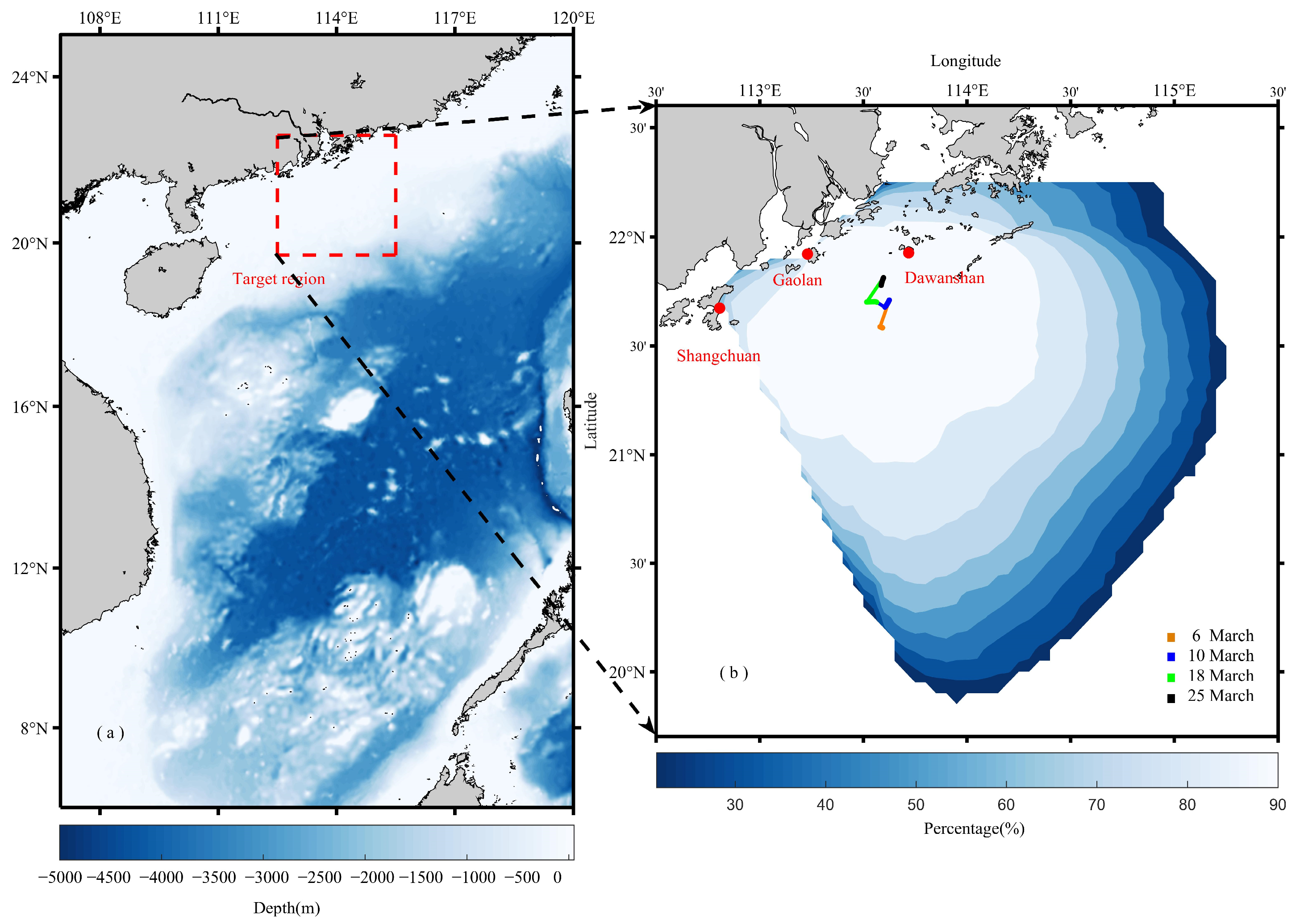
2.1. HFSWRS Observation Data

The three-station HFSWRS, including Shangchuan Island Radar Station (21.6733°N, 112.8067°E), Dawanshan Radar Station (21.9261°N, 113.7183°E) and Gaolan Island Radar Station (21.9208°N, 113.2304°E), is located at the adjacent waters of the Pearl River Estuary (Figure 1a) and used to observe the sea surface currents.
Gaolan Island Radar Station was constructed in 2018. Gaolan Island Radar Station is equipped with the OSMAR071G all-digital HFSWRS, featuring a single transmitting antenna. It employs eight receiving antennas arranged in a dual-row setup: six in the front row along the breakwater guardrail and two in the rear row. Operating at a center frequency of 8.115 MHz, the radar system covers a 200° sector with a maximum detection range of 250 km. The Dawanshan and Shangchuan stations were also equipped with OSMAR071G all-digital HFSWRS, and are operated at a nominal frequency of 9 MHz. Each station formed an antenna array, consisting of a minimum of three transmitting antennas and eight or more receiving antennas. The details on the equipment parameters and observation principles for the Dawanshan and Shangchuan stations are described in Zhu et al. [24]. The three-station HFSWRS collectively spans an extensive marine area of approximately 20,000 square kilometers. The radar data acquisition involves transmitting electromagnetic waves towards the sea surface. The backscattered ocean echoes are received by the antenna array, with the receiving module performing filtering, amplification, and digitalization. Processed data, obtained through computer terminal sampling software, undergoes further analysis using the SeaMonitor software with the MUSIC algorithm [35]. The data from the Gaolan Island Radar Station is uploaded to a synthesis station, where it merges with data from the other two radar stations. This synthesis process yields comprehensive vector flow field and wind-wave field data for the monitored sea area, enhancing the accuracy and reliability of observations. The HFSWRS methodology ensures real-time detection of the flow field over a large sea area, providing valuable insights into oceanic processes.
The period of the three-station HFSWRS observation used in this study spans from 5 March 2019 to 13 April 2019. The data were collected with a sampling interval of 20 min and a spatial resolution of 0.05° × 0.05°. Theoretically, there are 2819 spatial points. However, gaps exist in both spatial and temporal coverage. The temporal coverage percentage at spatial points ranges from 25% to 90% (Figure 1b). We selected spatial points where the observation covers over 60% of the period, resulting in 1085 spatial points available for analysis.
The three-station HFSWRS observation was first validated by the underway measurements of the sea surface currents obtained by using an ADCP installed on a moving ship in the spring of 2019. The trajectories of the underway measurements are shown in Figure 1b. Compared to the commonly used two-station HFSWRS observation, the sea surface current velocity and direction observed by the three-station HFSWRS are much closer to the underway measurements, as shown in Figure 2. As listed in Table 1, the root mean squared errors (RMSEs) of the current velocity decreased from 7.43 cm/s on 6 March, 6.92 cm/s on 10 March, 3.39 cm/s on 18 March, and 6.63 cm/s on 25 March to 2.61 cm/s, 4.47 cm/s, 2.98 cm/s, and 4.00 cm/s, respectively. On the whole, the RMSEs of the current velocity and the current direction decreased by 42.86% and 38.30%, respectively, demonstrating better performance of the three-station HFSWRS in the core observation area. It should be pointed out that the observations near the edge of the observation area may be inaccurate due to insufficient coverage, which would be further evaluated by in situ observations in the future.

2.2. Harmonic Analysis

If the current is decomposed along the east and north directions, the east–west current velocity and south–north current velocity can also be regarded as the result of multiple components [36]:
U ( t ) = U 0 + k = 1 K f k ( t ) A k c o s V k ( t ) + u k ( t ) g k + R ( t ) = U 0 + i = 1 N N R f i ( t ) A i c o s V i ( t ) + u i ( t ) g i + R ( t ) + j = 1 N R   f j ( t ) A j c o s V j ( t ) + u j ( t ) g j + I = 1 N I f I ( t ) A I c o s V I ( t ) + u I ( t ) g I
where U ( t ) is the east–west current velocity (south–north current velocity); U 0 is the mean current velocity. The amplitude and phase lag (referred to Beijing standard time, the same below) are denoted by A and g, respectively. The nodal corrections to amplitude and phase lag are represented by f and u, respectively. Other variables include V for the astronomical argument, R for the nontidal component, K for the number of tidal constituents, NNR for the number of non-reference constituents, NR for the number of reference constituents, and NI for the number of constituents to be inferred from the jth reference constituents.
The harmonic analysis was performed using the widely used Matlab package U_tide [36], which can analyze the time series of observations with irregularly distributed temporal sampling. Because the diurnal constitutes K1 and P1 are close in frequency, which are 0.0418 and 0.0416 cycles per hour (cph) [37,38], it is unable to resolve K1 and P1 by directly analyzing the 40-day observations [39]. Similarly, S2 and K2 are close in the semi-diurnal band and cannot be resolved by analyzing the 40-day observations. In accordance with the Rayleigh criterion, an examination was conducted on four key tidal constituents (M2, S2, K1, and O1), as well as three shallow water constituents (M4, MS4, and M6). Moreover, the undetermined elements P1 and K2 were deduced from K1 and S2, correspondingly, using the inference parameters calculated with the harmonic constants acquired through the Tidal Inversion Software developed by Oregon State University [40].

3. Results

3.1. Tidal Current Ellipse

The tidal current ellipse parameters for the major semi-diurnal constituents M2 and S2, as well as the significant diurnal constituents K1 and O1, were obtained through a harmonic analysis of sea surface current data. Additionally, parameters for the shallow water constituents M4, MS4, and M6 in the region were obtained. These parameters are listed in Table 2. The M2 tidal component has the largest semi-major axis of 9.36 cm/s, indicating that the M2 tidal current takes a dominant role. The K1 tidal component is the second largest with a semi-major axis of 7.39 cm/s, while the S2 and O1 tidal components have smaller semi-major axes of 4.57 cm/s and 4.92 cm/s, respectively. The semi-minor axes of all tides are significantly smaller than their semi-major axes. The inclination angles of the M2, K1, and S2 tidal components are all between 130° and 150°, indicating that the predominant tidal motion is a back-and-forth flow in the northwest–southeast direction with a tendency towards onshore–offshore flow.
The determination of tidal current rotation is based on the ellipticity (K) of the tidal current ellipses, where K signifies the ratio of the minor axis to the major axis of the tidal ellipse [41]. When the mean value of |K| is less than 0.3, the reciprocating flow is significant. When the mean value of |K| is larger than 0.3, the rotating flow is significant; moreover, it tends to become circular when the mean value of |K| approaches 1. Within this study, the wide range of K values for the tidal components implies diverse tidal current patterns in the region, encompassing both rotating and reciprocating flows, rather than being confined to a singular flow pattern. For the seven tidal components mentioned above, the mean values of |K| are all less than 0.3, indicating that the predominant motion is primarily back-and-forth flow.
The tidal ellipses of the four major tidal components M2, S2, K1, and O1 are shown in Figure 3. Although the mean values of K for each tidal component in the entire region are relatively small, the patterns of tidal motion vary from place to place. From Figure 3a, it can be seen that the M2 constituent displays features of back-and-forth flow in the northwest–southeast direction in most areas, with inclination angles generally perpendicular to the coastline. Close to the Pearl River Estuary’s entrance, the M2 tidal ellipses are more circular with smaller inclination angles and significantly increased velocity. Circular tidal ellipses also occur in the southeastern part of the region. Figure 3b shows that the S2 constituent has a smaller flow velocity than the M2 constituent, with a similar pattern. In the central part of the observed area, it is a back-and-forth flow in the northwest–southeast direction. Near the mouth of the Pearl River and the Modaomen River in the north, the tidal ellipses appear more circular. In a southern part of the observed area, and far from the coastline, the sea currents exhibit rotational characteristics. As shown in Figure 3c, the K1 constituent exhibits a coexistence of rotational and back-and-forth flow patterns. The flow velocity is significantly higher near the coastline and decreases with increasing distance from the coastline. The tidal ellipses mainly show a northwest–southeast orientation, but there is a change in inclination angle at the southern end of the observed area, exhibiting a southwest–northeast flow direction. Because the major axis of the K1 tidal ellipse is larger than that of the S2 tidal ellipse, the K1 constituent has a greater influence on the overall tidal current, only smaller than the M2 constituent. Figure 3d shows that the flow velocity of the O1 constituent is smaller than the K1 constituent, indicating that the O1 constituent has a relatively smaller influence within the diurnal tidal components. The O1 constituent mainly flows in a northwest–southeast direction and exhibits a back-and-forth flow in an east–west direction in the southern end of the observed area.
The tidal ellipses of the shallow water constituents are shown in Figure 4. The flow velocity of the shallow water constituents is significantly smaller than that of the four major tidal components, and their motion patterns are relatively consistent. The western and central parts of the observed area exhibit an east–west back-and-forth flow, while in the eastern part, farther away from the coastline, the direction of the tidal flow transitions to the southwest–northeast direction. The flow velocity significantly increases near the coast, and the flow direction is primarily perpendicular to the coastline, exhibiting a rotational flow motion pattern.

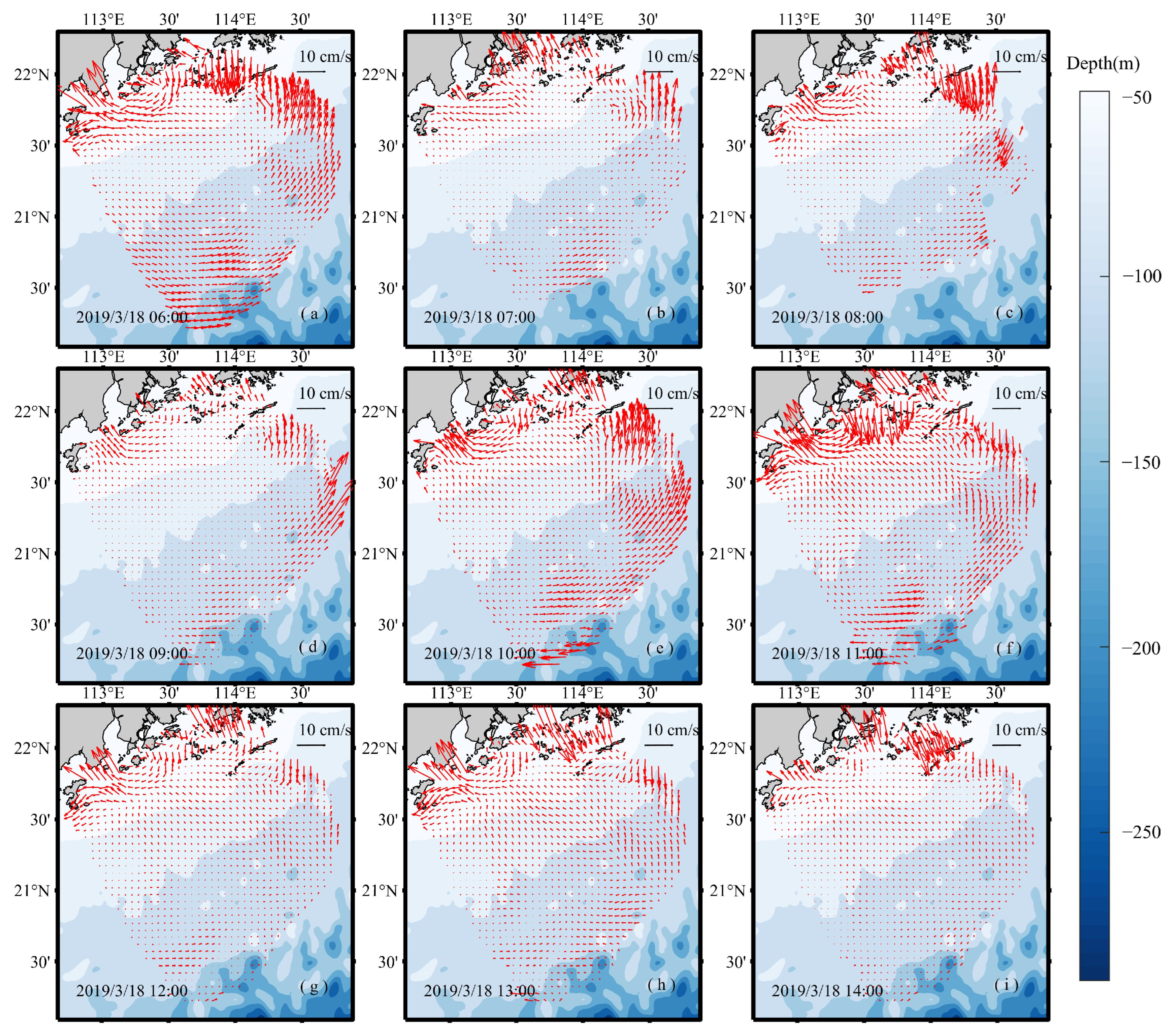
3.2. Tidal Current Pattern

The tidal type F = W O 1 + W K 1 / W M 2 , where W O 1 , W K 1 , W M 2 are the semi-major axes of tidal current ellipse of O1, K1, M2, correspondingly, is calculated. In addition, the shallow water constituent coefficient G = W M 4 + W M S 4 / W M 2 is calculated, where W M 4 and W M S 4 are the semi-major axes of the tidal current ellipse of M4 and MS4, respectively. Figure 5 provides the spatial representations of tidal current patterns and the impact of shallow water constituents within the adjacent waters of the Pearl River Estuary.
It can be seen from Figure 5a that the minimum F value in this region was 0.68, with 83.87% of observed points falling between 0.68 and 2, suggesting that the tidal current characteristics in this region follow an irregular semi-diurnal pattern. The unusually high values (approximately 8) of F observed at the northwestern boundary may be attributed to inaccuracies in the radar data or the distinctive topography of that particular region. In Figure 5b, all radar cells exhibit G values surpassing 0.02, suggesting a significant effect of shallow water constituents in the study area, which aligns with prior research findings [33].

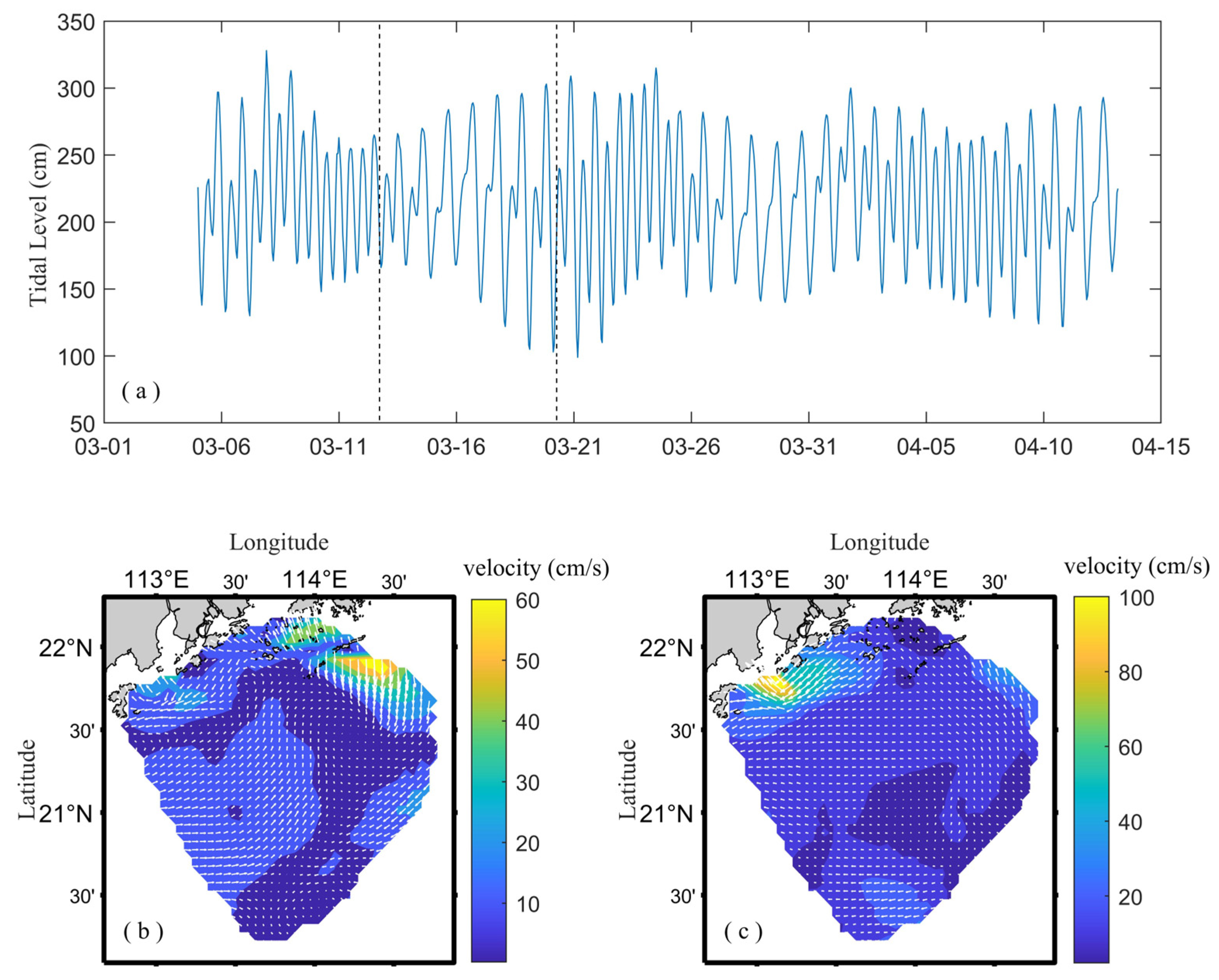
3.3. Daily Averaged Flow Field during Spring and Neap Tide

Based on the tidal-level data at Dawanshan Station, the tidal range reaches its minimum on 12 March, which is chosen as the representative day for the neap tide. Meanwhile, the tidal range reaches its maximum on 20 March, which is chosen as the representative day for spring tide. Daily averaged sea surface currents are shown in Figure 6. On the representative day for the spring tides, the current direction at observation points near the northwest coast is perpendicular to the coastline. Due to the blocking effect of the coastline and islands, local sea surface currents flow southwest along the coastline. The southwest and central regions of the study area show northward flow, while sea surface currents in the northeast are influenced by the environment and flow southward. On the representative day for the neap tides, the sea surface current direction in the observed area is generally from east to west, with significantly increased current velocity near the coast.

3.4. Tidal Energy

Tidal energy flux is a variable that is influenced by various factors such as terrains and hydrodynamic environments. In this study, tidal energy flux E refers to the sum of tidal potential energy and kinetic energy, with units of W/m. The formula of tidal energy flux is as follows [42]:
E = 1 T 0 T ( U 2 2 + g z ) ρ H U d t
where the velocity vector is denoted as U , and g represents the acceleration due to gravity, exhibiting slight variations with latitude. T is the tidal current variation period, H represents the water depth at the calculation point, ρ is the density of seawater and taken as 1020 kg/m3, and z is the tidal-level variation at the point. Since we cannot obtain tidal-level data for every observation point in the observed area of the three-station HFSWRS, the tidal-level data at Dawanshan Station are used to represent the tidal-level variation in the entire observed area. A synodic month is approximately 30 days, so this study uses data from March 5 to April 4, which include both spring and neap tides. The temporally averaged tidal energy can be considered as representative for a steady state and is shown in Figure 7.
From Figure 7, it can be seen that tidal energy near the Pearl River Estuary is primarily brought in from the eastern continental shelf and the southeastern region. The overall direction is mainly from the east to the west, and the maximum value is 9.70 × 10⁴ W/m. In the northern part of the observation area, the tidal energy flux at the observation points decreases. There are two main reasons for this phenomenon. Firstly, the shallow water depth in the northern part leads to a decrease in the potential energy flux of tidal energy. Secondly, the clustered islands have an impact on tidal energy flux. The presence of islands near the coast obstructs tidal flow, causing tidal waves to converge and accumulate around the islands. As a result, a complex tidal flow field emerges. In such cases, tidal energy in the vicinity of the islands would be influenced, leading to a decrease in tidal energy flux. Additionally, factors such as the topography of the sea area also influence the distribution of tidal energy flux. In the western coastal area, the propagation direction of tidal energy flux deviates along the coastline, which has not been observed in previous studies. The HFSWRS can provide a more detailed description of tidal energy variations within small-scale areas while revealing the distribution of tidal energy in the study area.

3.5. Residual Current Characteristics

As the residual currents significantly contribute to the dispersion and diffusion of suspended and soluble matter in the ocean, the residual currents are calculated by subtracting the periodic tidal currents from the observed current and are studied. The periodic tidal currents are reconstructed by substituting the harmonic constants of the tidal constituents obtained in harmonic analysis into the right side of Equation (1). As shown in Figure 8c,d, there are differences between the observed velocity data and the reconstructed tidal currents at point P, especially in the east–west direction, indicating that the residual current in the east–west direction is prominent. The wind velocity at point P was obtained from Copernicus Climate Change Service (C3S) Climate Data Store (CDS) [43] and is shown in Figure 8b. The reconstructed tidal currents of the north–south component align well with the observed velocity. The calculated correlation coefficient for residual current velocity and wind velocity remains at 0.35, indicating a discernible positive correlation between them, as depicted in Figure 9a. In the east–west direction (Figure 9b), the residual current is strongly correlated with the wind. The correlation coefficient between the residual currents and wind is 0.63, indicating that residual currents and wind are highly correlated. The direction of the residual currents is basically consistent with the wind direction. In addition, the variations in residual current velocity and wind velocity are also consistent, demonstrating that the residual current in the observed area is mainly affected by the wind.
Figure 10 displays the hourly residual current field from 6:00 to 14:00 on March 18. The residual currents in the observed area exhibit a general pattern of being larger near the coast and smaller offshore. Although the residual current velocity increases at 10:00 and 11:00 in the offshore region, considering the influence of wind, the abnormal magnitude and uniform direction of the residual current velocity can be attributed to the effect of wind. The nearshore currents, on the other hand, exhibit chaotic directions and significant variations in velocity. This is due to the shallow water depth and clustered islands near the coast, which significantly affect the currents.

4. Discussion and Conclusions

By analyzing the sea surface current observed by the three-station HFSWRS near the Pearl River Estuary, the tidal current characteristics in the observed area are obtained.
(1)
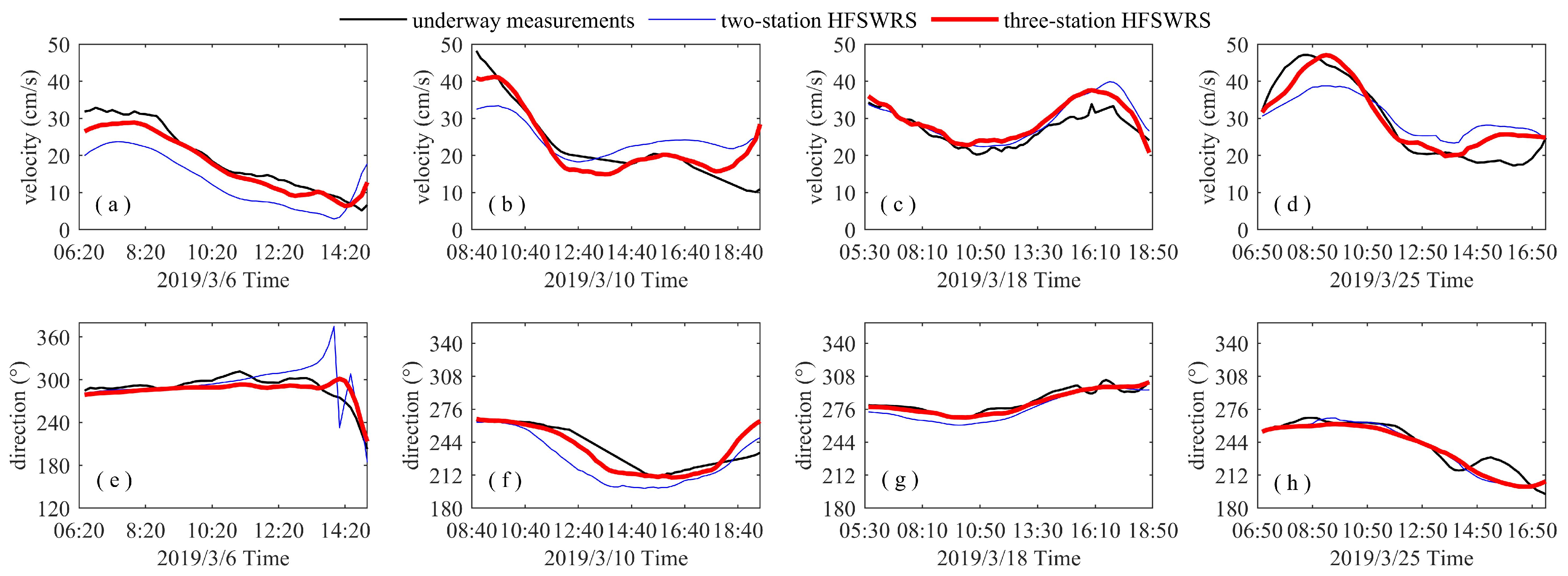
Compared to the two-station HFSWRS, the deviation of the current velocity and direction observed by the three-station HFSWRS from the underway measurements decreased by 42.86% and 38.30%, respectively.
(2)
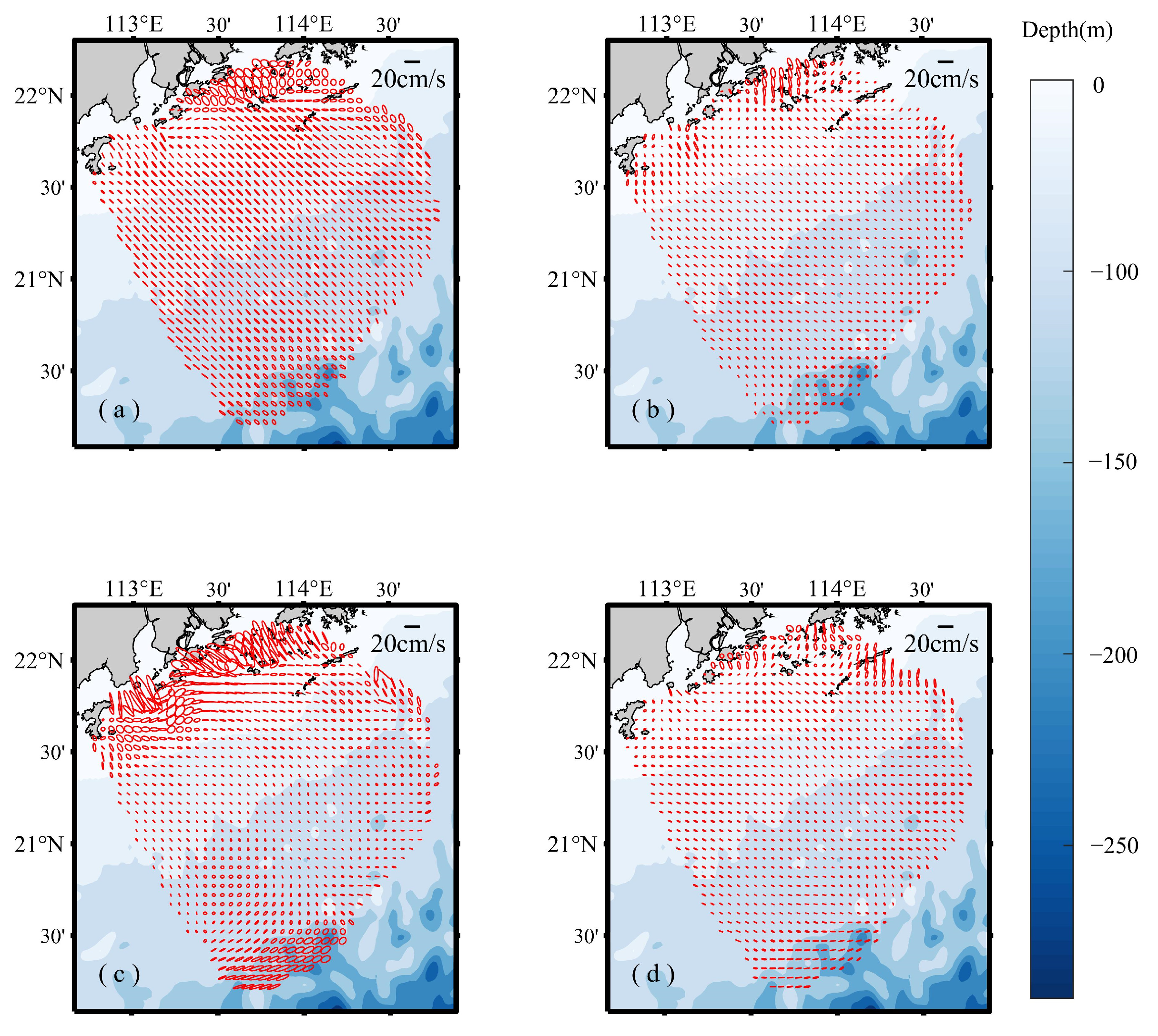
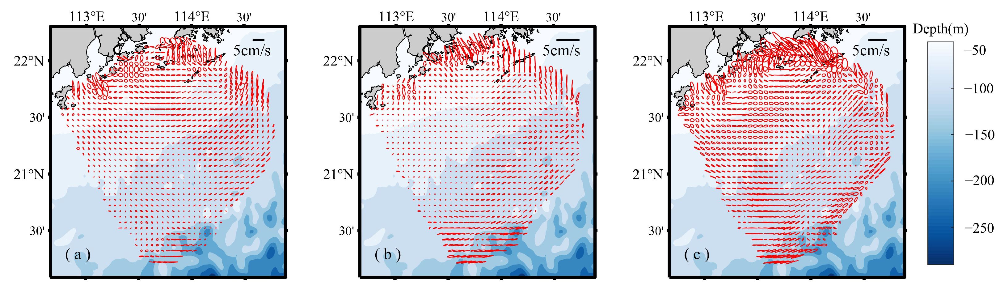
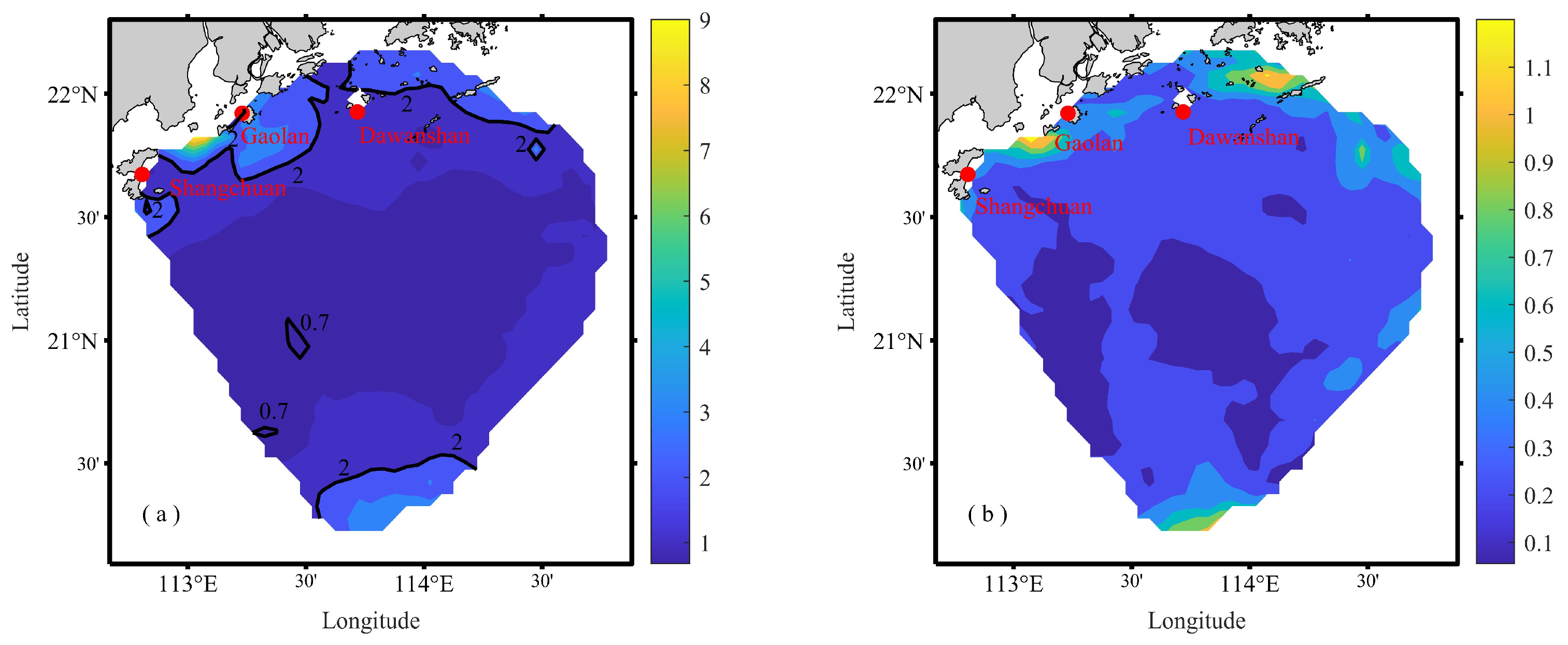
Through the analysis of the tidal ellipse parameters and tidal ellipse figures in the region, it was found that the dominant constituents in the area are the M2 and K1 tides, followed by the O1 and S2 tides. The flow velocity of each constituent generally increases near the coast. Based on the mean ellipticity of the tidal ellipses, it was found that the predominant motion is primarily a back-and-forth flow. The flow varies from place to place, often showing a more circular pattern near the coast.
(3)
By calculating the coefficients of the tidal type and the shallow water constituent at the observation points, it was revealed that the region is primarily influenced by irregular semi-diurnal tides, but near the coast, the tidal currents exhibit characteristics of diurnal tides due to factors such as topography. The impact of shallow water constituents in this region is noteworthy.
(4)
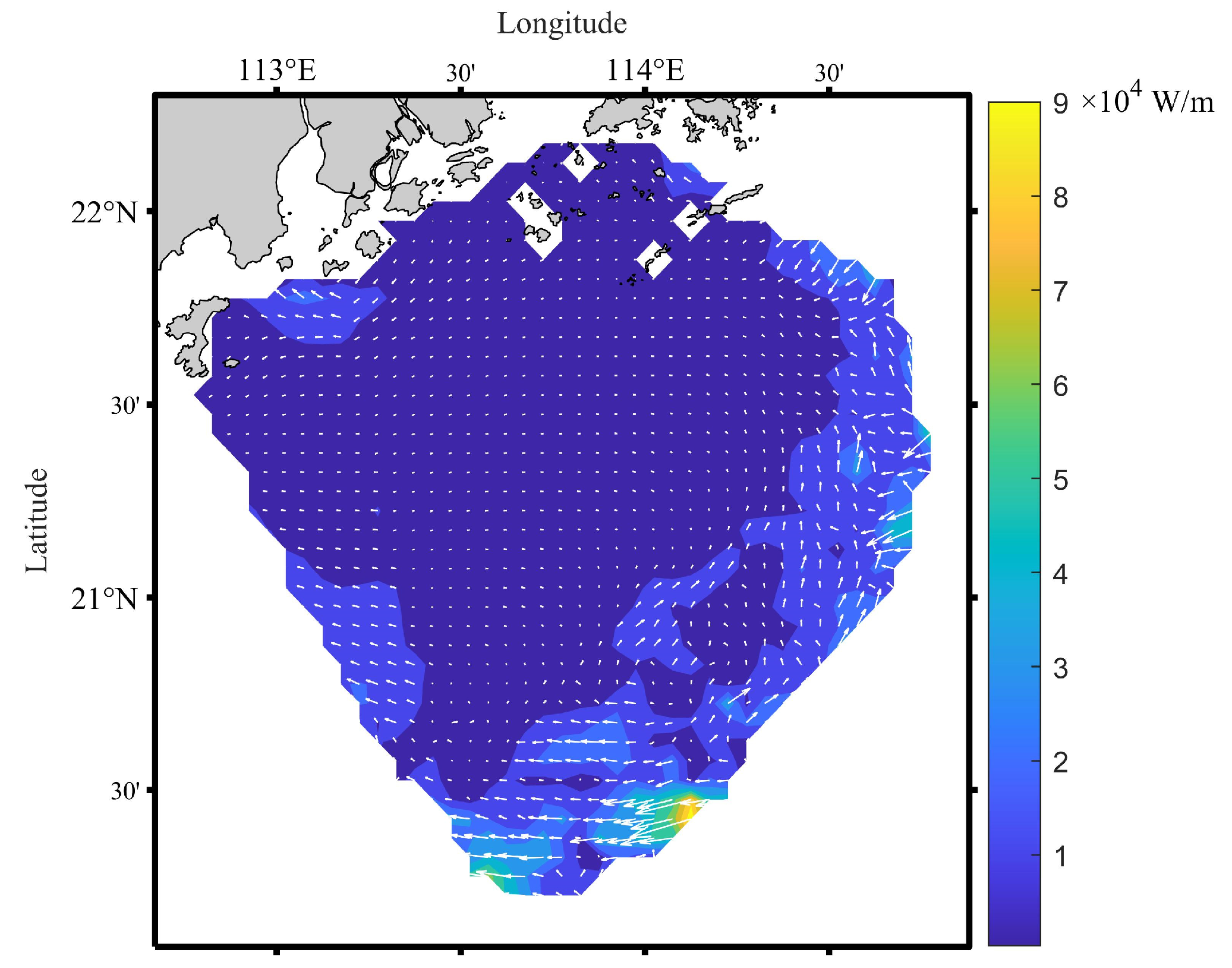
The tidal energy flux in the study area generally propagates from southeast to northwest. In nearshore areas, the direction of propagation tends to refract toward the shore, and the magnitude of the tidal energy flux decreases in the northern part of the study area.
(5)
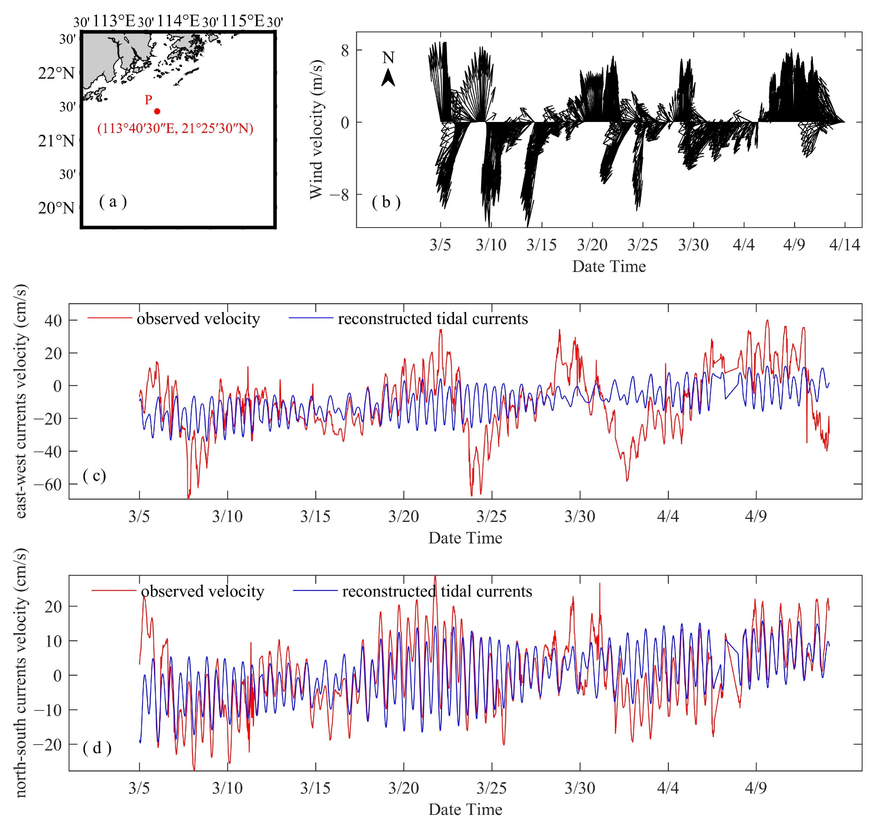
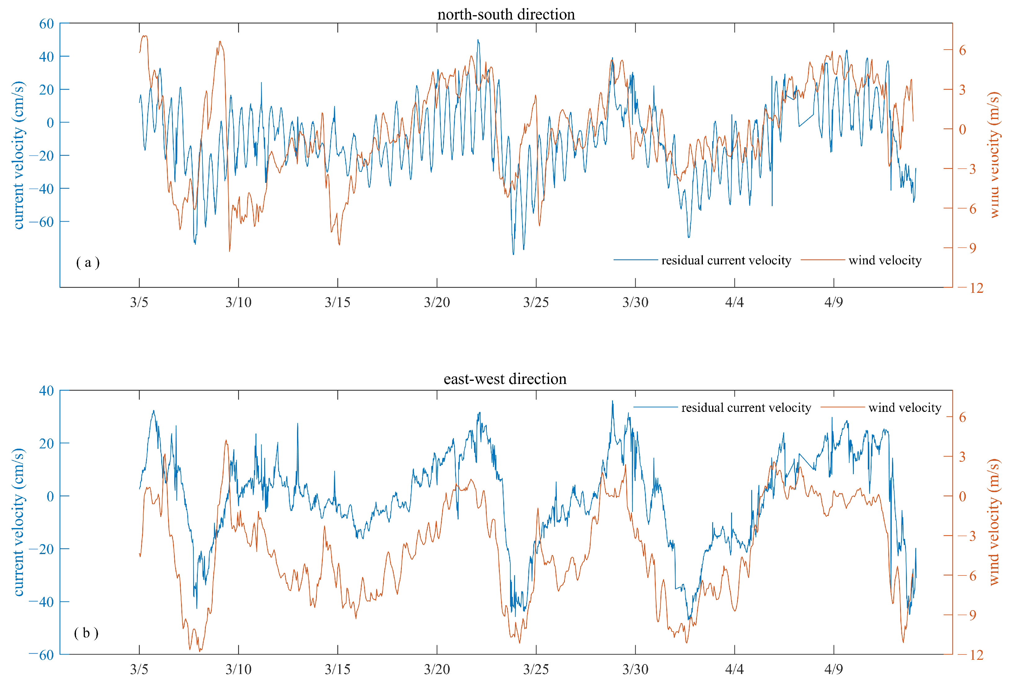
The analysis of the residual current field and wind field at point P suggests that the residual currents at that location are influenced by wind, and the residual current field indicates that nearshore residual currents are also significantly affected by topography.
As shown by Zhu et al. [24], a new radar observing network with about 10 radar stations is developing in the Pearl River Estuary and its adjacent shelf. Based on the newly established Gaolan Island Radar Station, the accuracy using three-station HFSWRS is evaluated and firstly used to study the sea surface current in this study. The accuracy of the current observed by the three-station HFSWRS is improved, compared with that of using two-station HFSWRS, which is attributed to the expanded overlap coverage of the radar observing system. In addition, the HFSWRS is the most effective way to observe the sea surface current with wide spatial coverage and high temporal resolution. Therefore, this study provides important reference and confidence for the application of the developing new radar observing network with about 10 radar stations.
While previous studies have addressed tidal current ellipses and parameters associated with major constituents in this area, this study delves more profoundly into the influence of shallow water constituents and residual currents. It is noted that the analyzed observations were only carried out in spring, so many more observations will be analyzed to explore seasonal variations, contributing to a more profound comprehension of the tidal dynamics in this region. In addition, the sea surface current data obtained from the multiple-station HFSWRS will be assimilated into numerical models in the future to improve the prediction capabilities and to gain a more complete understanding of the complex ocean dynamical processes.

Author Contributions

Conceptualization, D.W.; funding acquisition, D.W. and L.M.; investigation, H.L., L.Z. and D.W.; methodology, H.L. and D.W.; software, L.Z. and D.W.; visualization, H.L.; writing—original draft, H.L.; writing—review and editing, L.Z., D.W. and L.M. All authors have read and agreed to the published version of the manuscript.

Funding

This research was funded by Open Funds for Key Laboratory of Marine Environmental Survey Technology and Application, Ministry of Natural Resources (grant number MESTA-2021-A004), the Fund of Guangxi Key Laboratory of Beibu Gulf Marine Resources, Environment and Sustainable Development (grant number MRESD-2023-B02), Guangdong Basic and Applied Basic Research Foundation (grant number 2023A1515011262), and the National Natural Science Foundation of China (grant number 42106033, 42176172, 41876086).

Data Availability Statement

Not applicable.

Conflicts of Interest

The authors declare no conflicts of interest.

References

  1. Lana, A.; Marmain, J.; Fernández, V.; Tintoré, J.; Orfila, A. Wind influence on surface current variability in the Ibiza Channel from HF Radar. Ocean Dyn. 2016, 66, 483–497. [Google Scholar] [CrossRef]
  2. Ma, Y.; Yin, W.; Guo, Z.; Xuan, J. The Ocean Surface Current in the East China Sea Computed by the Geostationary Ocean Color Imager Satellite. Remote Sens. Online 2023, 15, 2210. [Google Scholar] [CrossRef]
  3. Griffiths, S.D.; Grimshaw, R.H.J. Internal Tide Generation at the Continental Shelf Modeled Using a Modal Decomposition: Two-Dimensional Results. J. Phys. Oceanogr. 2007, 37, 428–451. [Google Scholar] [CrossRef]
  4. Echeverri, P.; Peacock, T. Internal tide generation by arbitrary two-dimensional topography. J. Fluid Mech. 2010, 659, 247–266. [Google Scholar] [CrossRef]
  5. Xu, J.; Zhang, Y.; Cao, A.; Liu, Q.; Lv, X. Effects of tide-surge interactions on storm surges along the coast of the Bohai Sea, Yellow Sea, and East China Sea. Sci. China Earth Sci. 2016, 59, 1308–1316. [Google Scholar] [CrossRef]
  6. Wang, Y.; Duan, Y.; Guo, Z.; Chen, W.; Zhang, X.; Han, Z. Deterministic-probabilistic approach for probable maximum typhoon-induced storm surge evaluation over Wenchang in the South China sea. Estuar. Coast. Shelf Sci. 2018, 214, 161–172. [Google Scholar]
  7. Munk, W.; Wunsch, C. Abyssal recipes II: Energetics of tidal and wind mixing. Deep. Sea Res. Part I Oceanogr. Res. Pap. 1998, 45, 1977–2010. [Google Scholar] [CrossRef]
  8. Kido, M.; Imano, M.; Ohta, Y.; Fukuda, T.; Takahashi, N.; Tsubone, S.; Ishihara, Y.; Ochi, H.; Imai, K.; Honsho, C.; et al. Onboard Realtime Processing of GPS-Acoustic Data for Moored Buoy-Based Observation. J. Disaster Res. 2018, 13, 472–488. [Google Scholar] [CrossRef]
  9. O’Reilly, W.C.; Olfe, C.B.; Thomas, J.; Seymour, R.J.; Guza, R.T. The California coastal wave monitoring and prediction system. Coast. Eng. 2016, 116, 118–132. [Google Scholar] [CrossRef]
  10. Zhenhua, J.; Maochong, S.; Jijun, S. Prediction of ocean surface current velocity and application to meteorological navigation in the North Pacific. Chin. J. Oceanol. Limnol. 1990, 8, 1–25. [Google Scholar] [CrossRef]
  11. Guo, P.; Fang, W.; Liu, C.; Qiu, F. Seasonal characteristics of internal tides on the continental shelf in the northern South China Sea. J. Geophys. Res. Ocean. 2012, 117, C04023. [Google Scholar] [CrossRef]
  12. Chaigneau, A.; Dominguez, N.; Eldin, G.; Vasquez, L.; Flores, R.; Grados, C.; Echevin, V. Near-coastal circulation in the Northern Humboldt Current System from shipboard ADCP data. J. Geophys. Res. Ocean. 2013, 118, 5251–5266. [Google Scholar] [CrossRef]
  13. Mazzega, P.; Bergé, M. Ocean tides in the Asian semienclosed seas from TOPEX/POSEIDON. J. Geophys. Res. Ocean. 1994, 99, 24867–24881. [Google Scholar] [CrossRef]
  14. Zhao, J.; Chen, X.; Hu, W.; Chen, J.; Guo, M. Dynamics of surface currents over Qingdao coastal waters in August 2008. J. Geophys. Res. Ocean. 2011, 116, C10020. [Google Scholar] [CrossRef]
  15. Hickey, K.J.; Gill, E.W.; Helbig, J.A.; Walsh, J. Measurement of ocean surface currents using a long-range, high-frequency ground wave radar. IEEE J. Ocean. Eng. 1994, 19, 549–554. [Google Scholar] [CrossRef]
  16. Garraffo, Z.D.; Mariano, A.J.; Griffa, A.; Veneziani, C.; Chassignet, E.P. Lagrangian data in a high-resolution numerical simulation of the North Atlantic: I. Comparison with in situ drifter data. J. Mar. Syst. 2001, 29, 157–176. [Google Scholar] [CrossRef]
  17. Han, S.; Yang, H.; Xue, W.; Wang, X. The study of single station inverting the sea surface current by HF ground wave radar based on adjoint assimilation technology. J. Ocean Univ. China 2017, 16, 383–388. [Google Scholar] [CrossRef]
  18. Barrick, D. First-order theory and analysis of MF/HF/VHF scatter from the sea. IEEE Trans. Antennas Propag. 1972, 20, 2–10. [Google Scholar] [CrossRef]
  19. Barrick, D.E.; Evans, M.W.; Weber, B.L. Ocean Surface Currents Mapped by Radar. Science 1977, 198, 138–144. [Google Scholar] [CrossRef]
  20. Lipa, B.; Barrick, D. Tidal and storm-surge measurements with single-site CODAR. IEEE J. Ocean. Eng. 1986, 11, 241–245. [Google Scholar] [CrossRef]
  21. Shay, L.K.; Martinez-Pedraja, J.; Cook, T.M.; Haus, B.K.; Weisberg, R.H. High-Frequency Radar Mapping of Surface Currents Using WERA. J. Atmos. Ocean. Technol. 2007, 24, 484–503. [Google Scholar] [CrossRef]
  22. Lorente, P.; Soto-Navarro, J.; Alvarez Fanjul, E.; Piedracoba, S. Accuracy assessment of high frequency radar current measurements in the Strait of Gibraltar. J. Oper. Oceanogr. 2014, 7, 59–73. [Google Scholar] [CrossRef]
  23. Capodici, F.; Cosoli, S.; Ciraolo, G.; Nasello, C.; Maltese, A.; Poulain, P.-M.; Drago, A.; Azzopardi, J.; Gauci, A. Validation of HF radar sea surface currents in the Malta-Sicily Channel. Remote Sens. Environ. 2019, 225, 65–76. [Google Scholar] [CrossRef]
  24. Zhu, L.; Lu, T.; Yang, F.; Liu, B.; Wu, L.; Wei, J. Comparisons of Tidal Currents in the Pearl River Estuary between High-Frequency Radar Data and Model Simulations. Appl. Sci. 2022, 12, 6509. [Google Scholar] [CrossRef]
  25. Barrick, D. History, present status, and future directions of HF surface-wave radars in the U.S. In Proceedings of the 2003 Proceedings of the International Conference on Radar (IEEE Cat. No.03EX695), Adelaide, SA, Australia, 3–5 September 2003; pp. 652–655. [Google Scholar]
  26. Lan, W.; Huang, B.; Dai, M.; Ning, X.; Huang, L.; Hong, H. Dynamics of heterotrophic dinoflagellates off the Pearl River Estuary, northern South China Sea. Estuar. Coast. Shelf Sci. 2009, 85, 422–430. [Google Scholar] [CrossRef]
  27. Lyu, S.; Deng, S.; Lin, K.; Zeng, J.; Wang, X. Designing and the Pilot Trial of Bivalve Molluscan Fishing Quotas on Maoming Coastal Waters of China, Northern South China Sea. Front. Mar. Sci. 2022, 9, 863376. [Google Scholar] [CrossRef]
  28. Fu, Y.; Zhou, D.; Zhou, X.; Sun, Y.; Li, F.; Sun, W. Evaluation of satellite-derived tidal constituents in the South China Sea by adopting the most suitable geophysical correction models. J. Oceanogr. 2020, 76, 183–196. [Google Scholar] [CrossRef]
  29. Xinglong, K.; Wenyan, H.; Yuge, Z. Research on the Development of Marine Tourism Industry and Talent Demand in Guangdong-Hong Kong-Macao Greater Bay Area. In Proceedings of the 2020 International Conference on Management, Economy and Law (ICMEL 2020), Zhengzhou, China, 22–23 September 2020; Atlantis Press: Paris, Franch, 2020; pp. 292–297. [Google Scholar]
  30. Hu, S.; Liu, B.; Hu, M.; Yu, X.; Deng, Z.; Zeng, H.; Zhang, M.; Li, D. Quantification of the nonlinear interaction among the tide, surge and river in Pearl River Estuary. Estuar. Coast. Shelf Sci. 2023, 290, 108415. [Google Scholar] [CrossRef]
  31. Cai, S.; Huang, Q.; Long, X. Three-dimensional numerical model study of the residual current in the South China Sea. Oceanol. Acta 2003, 26, 597–607. [Google Scholar] [CrossRef]
  32. Zhu, X.-H.; Ma, Y.-L.; Guo, X.; Fan, X.; Long, Y.; Yuan, Y.; Xuan, J.-L.; Huang, D. Tidal and residual currents in the Qiongzhou Strait estimated from shipboard ADCP data using a modified tidal harmonic analysis method. J. Geophys. Res. Ocean. 2014, 119, 8039–8060. [Google Scholar] [CrossRef]
  33. Lei, R.; Fan, Y.; Lingna, Y.; Xiaofan, C.; Guangwei, P.; Jun, W. Characteristics of Surface Currents in Guangdong-Hong Kong-Macao Greater Bay Area in Spring Based on High Frequency Radar Observations. Beijing Da Xue Xue Bao 2022, 58, 839–849. [Google Scholar]
  34. Hu, Z.; Li, H.; Wang, D. Characterizing Tidal Currents and Guangdong Coastal Current Over the Northern South China Sea Shelf Using Himawari-8 Geostationary Satellite Observations. Earth Space Sci. 2023, 10, e2023EA003047. [Google Scholar] [CrossRef]
  35. Yang, S.L.; Ke, H.Y.; Wen, B.Y.; Cheng, F.; Zhou, H. Postprocessing of Ocean Surface Radial Current Mapping of OSMAR2000. Wuhan Univ. J. (Nat. Sci. Ed.) 2001, 5, 614–617. [Google Scholar]
  36. Codiga, D. Unified Tidal Analysis and Prediction Using the UTide Matlab Functions. 2011. Available online: https://www.mathworks.com/matlabcentral/fileexchange/46523-utide-unified-tidal-analysis-and-prediction-functions (accessed on 11 October 2022).
  37. Wang, D.; Pan, H.; Jin, G.; Lv, X. Seasonal variation of the principal tidal constituents in the Bohai Sea. Ocean Sci. 2020, 16, 1–14. [Google Scholar] [CrossRef]
  38. Wei, Z.; Jiao, X.; Du, Y.; Zhang, J.; Pan, H.; Wang, G.; Wang, D.; Wang, Y.P. The temporal variations in principal and shallow-water tidal constituents and their application in tidal level calculation: An example in Zhoushan Archipelagoes with complex bathymetry. Ocean Coast. Manag. 2023, 237, 106516. [Google Scholar] [CrossRef]
  39. Guohong, F.; Ji, W. An analysis of the astrometeorological constituents of tide in the Bohai Sea. Acta Oceanol. Sin. 1986, 4, 486–495. [Google Scholar]
  40. Egbert, G.D.; Erofeeva, S.Y. Efficient Inverse Modeling of Barotropic Ocean Tides. J. Atmos. Ocean. Technol. 2002, 19, 183–204. [Google Scholar] [CrossRef]
  41. Chen, Q.; Huang, D.; Zhang, B.; Wang, M. Characteristics of the tidal current and residual current in the seas adjacent to Zhejiang. Donghai Mar. Sci. 2003, 21, 1–14. [Google Scholar]
  42. Harari, J.; de Camargo, R. Numerical simulation of the tidal propagation in the coastal region of Santos (Brazil, 24°S 46°W). Cont. Shelf Res. 2003, 23, 1597–1613. [Google Scholar] [CrossRef]
  43. Hersbach, H.; Bell, B.; Berrisford, P.; Biavati, G.; Horányi, A.; Muñoz Sabater, J. ERA5 Hourly Data on Single Levels from 1979 to Present. Copernicus Climate Change Service (C3S) Climate Data Store (CDS). Available online: https://cds.climate.copernicus.eu/cdsapp#!/dataset/reanalysis-era5-single-levels (accessed on 7 February 2023).
Figure 1. (a) Location of the study area; (b) temporal coverage percentage of the valid observations at the observed area, location of the high-frequency surface wave radar stations (red dots), and trajectories of the underway measurements on 6 March (orange squares), 10 March (blue squares), 18 March (green squares), and 25 March (black squares), respectively.
Remotesensing 16 00672 g001
Figure 2. (ad) Sea surface current velocity and (eh) direction observed by the underway measurements (black lines), the two-station HFSWRS (blue lines), and three-station HFSWRS (red lines) in the spring of 2019.
Remotesensing 16 00672 g002
Figure 3. Tidal ellipses of (a) M2, (b) S2, (c) K1, and (d) O1.
Remotesensing 16 00672 g003
Figure 4. Tidal ellipses for (a) M4, (b) M6, and (c) MS4.
Remotesensing 16 00672 g004
Figure 5. Distribution of (a) tidal current type coefficient F and (b) shallow water constituent coefficient G. Contours of F values 0.7 and 2 are marked in (a).
Remotesensing 16 00672 g005
Figure 6. (a) Time series of the tidal level at Dawanshan Station, and spatial distribution of the daily averaged sea surface current during (b) the spring tide (20 March 2019) and (c) the neap tide (13 March 2019).
Remotesensing 16 00672 g006
Figure 7. Spatial distribution of tidal energy from 5 March 2019 to 4 April 2019.
Remotesensing 16 00672 g007
Figure 8. (a) Position of point P, (b) wind data at point P, (c) east-west current velocity from the observations (red line) and the reconstructed tidal components (blue line), and (d) same as (c) but for north–south current velocity.
Remotesensing 16 00672 g008
Figure 9. Time series of tidal residual current velocity (blue line) and wind velocity (red line) at Point P, with (a) representing the north–south direction and (b) depicting the east–west direction.
Remotesensing 16 00672 g009
Figure 10. Spatial distribution of tidal residual currents at (a) 6:00, (b) 7:00, (c) 8:00, (d) 9:00, (e) 10:00, (f) 11:00, (g) 12:00, (h) 13:00, and (i) 14:00 on 18 March 2019.
Remotesensing 16 00672 g010
Table 1. RMSEs of current velocity and direction between the underway measurements and two-station HFSWRS and those for three-station HFSWRS.
DateRMSEs of Current Velocity (cm/s)RMSEs of Current Direction (°)
Two-Station HFSWRSThree-Station HFSWRSTwo-Station HFSWRSThree-Station HFSWRS
6 March 20197.432.6120.5211.67
10 March 20196.924.4718.2510.72
18 March 20193.392.987.653.45
25 March 20196.634.008.808.69
Mean6.303.6014.919.20
Table 2. Tidal ellipse elements of the principal tidal constituents and shallow water constituents.
ConstituteSemi-Major Axis (cm/s)Semi-Minor Axis (cm/s)Inclination (°)Range of KMean of |K|
M29.361.57131.96−0.91~0.640.17
S24.571.07142.92−0.84~0.980.26
K17.391.91133.33−0.91~0.940.27
O14.921.1234.20−0.94~0.960.24
M41.430.32135.95−0.87~0.910.24
MS41.350.3323.98−0.79~0.950.26
M60.680.1233.41−0.87~0.920.22
Disclaimer/Publisher’s Note: The statements, opinions and data contained in all publications are solely those of the individual author(s) and contributor(s) and not of MDPI and/or the editor(s). MDPI and/or the editor(s) disclaim responsibility for any injury to people or property resulting from any ideas, methods, instructions or products referred to in the content.

