Parallel Spectral–Spatial Attention Network with Feature Redistribution Loss for Hyperspectral Change Detection

Abstract

Change detection methods using hyperspectral remote sensing can precisely identify differences of the same area at different observing times. However, due to massive spectral bands, current change detection methods are vulnerable to unrelatedspectral and spatial information in hyperspectral images with the stagewise calculation of attention maps. Besides, current change methods arrange hidden change features in a random distribution form, which cannot express a class-oriented discrimination in advance. Moreover, existent deep change methods have not fully considered the hierarchical features’ reuse and the fusion of the encoder–decoder framework. To better handle the mentioned existent problems, the parallel spectral–spatial attention network with feature redistribution loss (TFR-PS${}^2$ANet) is proposed. The contributions of this article are summarized as follows: (1) a parallel spectral–spatial attention module (${\mathrm{PS}}^2\mathrm{A}$) is introduced to enhance relevant information and suppress irrelevant information in parallel using spectral and spatial attention maps extracted from the original hyperspectral image patches; (2) the feature redistribution loss function (FRL) is introduced to construct the class-oriented feature distribution, which organizes the change features in advance and improves the discriminative abilities; (3) a two-branch encoder–decoder framework is developed to optimize the hierarchical transfer and change features’ fusion; Extensive experiments were carried out on several real datasets. The results show that the proposed ${\mathrm{PS}}^2\mathrm{A}$ can enhance significant information effectively and the FRL can optimize the class-oriented feature distribution. The proposed method outperforms most existent change detection methods.

1. Introduction

Hyperspectral remote sensing can capture subtle changes on the Earth’s surface because of its characteristic of high spectral resolution [1]. At present, technologies of hyperspectral change detection have been extensively applied in various domains, such as vegetation inspection, urban planning, and disaster monitoring [2,3,4,5]. Usually, change detection methods need plenty of training samples for effective and stable model results in different application scenes. The more training samples there are, the more stability the model can obtain. However, current change detection approaches are mostly designed for optical or multi-spectral images, which is a domain in which a model can be fed with sufficient training samples. This situation is in sharp contrast with the predicament of inadequate training samples in hyperspectral imaging. Furthermore, the data redundancy in both spectral and spatial information, mixed pixels caused by low spatial resolution, and the expensive change labeling for hyperspectral datasets make it difficult for multi-spectral change detection technologies to be transferred to hyperspectral images’ analysis [6].

Usually, the procedure of existent hyperspectral change detection methods can be divided into three different steps: the preprocessing of hyperspectral data, the usage of an appropriate change detection method, and the evaluation of the predicted change results:

(1) Data preprocessing: The preprocessing of hyperspectral images is the basic step for later change detection methods and greatly influences the effectiveness of the change detection results. A typical preprocessing includes registering of dual-temporal images and radiation correction to remove the effects of sunlight and the atmosphere.

(2) Change detection methods: An appropriate change detection method plays a critical role in the whole hyperspectral change detection procedure, which can directly influence the final performance indices. The selection or design of change detection methods needs to take the data structure of the preprocessed hyperspectral images into consideration, such as the remaining band number after noisy bands have been removed.

(3) Evaluation of the predicted change results: The prediction evaluation is the last step. Different evaluation indices can describe the performances of change detection methods from different viewpoints, such as the inference ability in the situation of imbalanced change types.

According to the order of appearance of change detection technologies, they can be categorized as traditional change detection methods and deep learning methods. In traditional change detection methods, based on the different procedures of the data processing, they can be further categorized as transformation-based approaches, algebra-based approaches, and independent image classification approaches. Basically, the main idea of transformation-based approaches is transforming temporal variants into another characteristic space to deal with information redundancy, but this makes it difficult for the model to decide on a proper threshold to precisely detect the changes, such as for change vector analysis (CVA) [7,8] and the similarity measure [9]. As for the algebra-based methods, they must handle the great computational cost due to the high-dimensional data structure. Regarding independent image classification, because the detection result is generated by processing two independent classification maps to produce a single change map, the result may be affected by the error propagation of both images’ classification results, which leads to bad performance.

The rapid development of deep learning methods has stimulated the evolution of hyperspectral change detection technologies. Compared to the traditional methods, the successful performance of deep learning models from other domains makes it possible to solve high-dimensional problems and extract extensive information more effectively. From the recent literature, deep learning methods can be roughly categorized into pixel-based methods and spatial–spectral-information-based methods. For pixel-wide scale analysis, researchers have contributed semi-supervised change detection frameworks, which are often composed of an encoder and a decoder to reconstruct the hyperspectral images by pixel spectral mapping. Then, the reconstructed images are distributed to downstream transformation methods and specific threshold segmentation methods, such as PCA and Otsu, to obtain the change map [10]. In this situation, the current methods consider deep learning as a preprocessing and compression step, but studies have not integrated the end-to-end change detection performance into a complete model, which results in the wasting of time and memory resources. Regarding the literature on feature extractors for both spectral and spatial information, existing methods propose the convolutional neural network to aggregate multi-direction information, by simply applying the conventional 2D spatial convolution on the compressed images or a direct 3D network to aggregate the two kinds of information at the same time [11,12,13]. Although these methods acknowledge that hyperspectral images themselves are equipped with various information, they still encounter bottlenecks that result from ignoring the spectral similarity in spatial areas and due to the insufficiency of hierarchical feature propagation. Furthermore, the local information usually can be distinguished by the relation to the global information, but current deep methods lack the ability to focus on the resemblance of spectral and spatial information simultaneously. The encoder–decoder framework in the literature was typically trained in a semi-supervised manner, which cannot hierarchically pass and fuse the features into deeper weight presentation to benefit change classification. Moreover, random features are distributed in fully connected layers, which are optimized by the later classification loss function and cannot be assigned for class judgment in advance. Therefore, these models’ drawbacks deeply hinder the improvement of current hyperspectral change detection methods’ performance.

To address these drawbacks of existing methods, in this paper, a parallel spectral–spatial attention network with feature redistribution loss in a supervised two-branch encoder–decoder framework is proposed for hyperspectral change detection. The proposed model rectifies the inner structure of the encoder–decoder framework so that it can be adopted in the proposed end-to-end model for transfer its original deep feature performance. Moreover, a weighted-in-parallel spectral–spatial attention module is constructed to focus on the long-range spectral and spatial dependencies within a patch’s input. To ensure that the fluent information flow can be fed into the classification function, an intensive module with multiple skip connections is applied. Furthermore, due to the unclear feature distribution’s influence in classification tasks [14], the feature redistribution loss function is developed here to provide better fused features for class-oriented loss computation.

The contributions of this paper are as follows:

(i) A parallel spectral–spatial attention module (${\mathrm{PS}}^2\mathrm{A}$) is proposed, which can provide the long-range dependenciesin the spectral domain and the local spatial region. Moreover, it fuses the separate stages of weighting the input data into a one-stage procedure, which can preserve the original data dependenciesand provide an enhancement in both the spectral and spatial domains at the same time.

(ii) The feature redistribution loss function (FRL) is developed for better feature arrangement. By maximizing the intra-group correlation and minimizing the extra-group correlation, a rectified loss function is developed, which helps the fused features form an enhanced distribution for class-oriented pattern recognition in advance. To ensure that fluent feature information for redistribution can be received, an intensive connected block (ICB) is applied with multiple skip connections between the convolutional submodules.

(iii) The encoder–decoder framework in a two-branch configuration is constructed in the end-to-end supervised change detection task. Although the decoder was not designed for pixel-level alignment, we found it quite effective to reuse its hierarchically transferred featuresfor change class prediction. This can largely contribute to the feature transfer by the skip connection and the fusion with the expanded feature reconstruction at a different scale.

Extensive experiments prove the effective and efficient performance of the presented method. The rest of this article is arranged as follows: Section 2 presents the related works on hyperspectral change detection methods. Section 3 introduces the proposed method. Section 4 gives the comparison result and ablation analysis of the proposed method. Section 5 is the conclusion of this study.

2. Related Works

2.1. Attention Mechanism

The attention mechanism was initially presented in the natural language processing domain, which is used to address the sequence-to-sequence transformation problem and is able to aggregate all the related information from the entire sequential input [15]. Along with the potential novelty and value of transferring the attention mechanism to computer vision applications, many works have created variants of the attention-based model for better effects in specific natural image analysis tasks. Among them, ViT is a prominent one, which reshapes the image patches into sequences and uses the attention mechanism in image classification [16]. Regarding object detection, DETR is another model that successfully explains the relation between the detected object and the global context to predict the final set of outputs in parallel [17]. Swin Transformer V2 is a model designed for semantic segmentation and uses the residual post-norm method to improve the training stability [18]. In the remote sensing change detection domain, Gong et al. proposed a spectral–spatial attention block to extract relevant information [11]. However, the generation of the attention map does not follow the standard weighting procedure, which may lead to inaccurate similarity computation. Qu et al. composed a dual-domain network to detect the change area from SAR images, which is based on the CNN architecture, and it can extract features at two different scales [19]. Wang et al. created a pyramid self-attention network to concentrate on features from different layers, but the training procedure followed a two-phrase auto-encoder framework and only applied dependency checks in the spatial domain [20]. Moreover, SSA-SiamNet, proposed by Wang et al., is an end-to-end model with a spectral–spatial attention mechanism. It uses a two-branch CNN feature extractor to generate gradually decreasing features for classification with a fully connected layer [21]. Applying the attention mechanism makes the extant models effective by emphasizing the spectral band and location relations while suppressing the unrelated information. Therefore, it is meaningful to take full advantage of the effectiveness of the attention mechanism in both the spectral and spatial domain.

2.2. Encoder–Decoder Framework

The encoder–decoder framework is a general method that generates an output sequence corresponding to an input sequence, and currently, it is being adopted in a variety of tasks such as semantic segmentation [22,23] and natural language processing [24,25]. In hyperspectral image analysis, most extant methods are designed according to the CNN or a dense prediction structure, such as GETNET and DSFANet [26,27], but there are still few studies on the supervised encoder–decoder framework. For hyperspectral classification, Zhu et al. created a spectral–spatial-dependent global learning framework, which utilizes the encoder–decoder structure to construct a pixel-level segmentation map [28]. For hyperspectral image reconstruction, Miao et al. developed a dual-stage generative model to reconstruct the desired 3D signal in snapshot compressive-spectral imaging. By applying U-Net to design a generative model, the 3D spectral cube can be directly reconstructed from the measurements and masks [29]. Huang et al. introduced a 3D filter generator, which can generate the spatially variant filters, into a lightweight U-Net for hyperspectral image reconstruction [30]. With the aim to address the conflicts of the dense sample tokens of the conventional Transformer model and the spatially sparse nature of hyperspectral image signals, Cai et al. developed a sparse Transformer (CST) model embedding HSI sparsity into deep learning for hyperspectral image reconstruction [31]. With respect to the application of the encoder–decoder structure in hyperspectral change detection, Lei et al. used the auto-encoder structure to learn the unsupervised patterns in the spectral pixel information by the definition of the reconstruction loss, then the reconstructed image was input into the later threshold segmentation procedure [10]. Due to the structure of hyperspectral images, the dimensionality reduction and data argumentation are usually used for the initial processing, and Li et al. adopted a two-branch U-Net network with feature fusion to achieve end-to-end change information detection automatically [32]. By adopting the encoder–decoder model in hyperspectral image analysis, current models can extend their potential to every specific research interest area. Therefore, it is necessary to improve the hierarchical feature transfer and fusion in the encoder–decoder networks for better application performances.

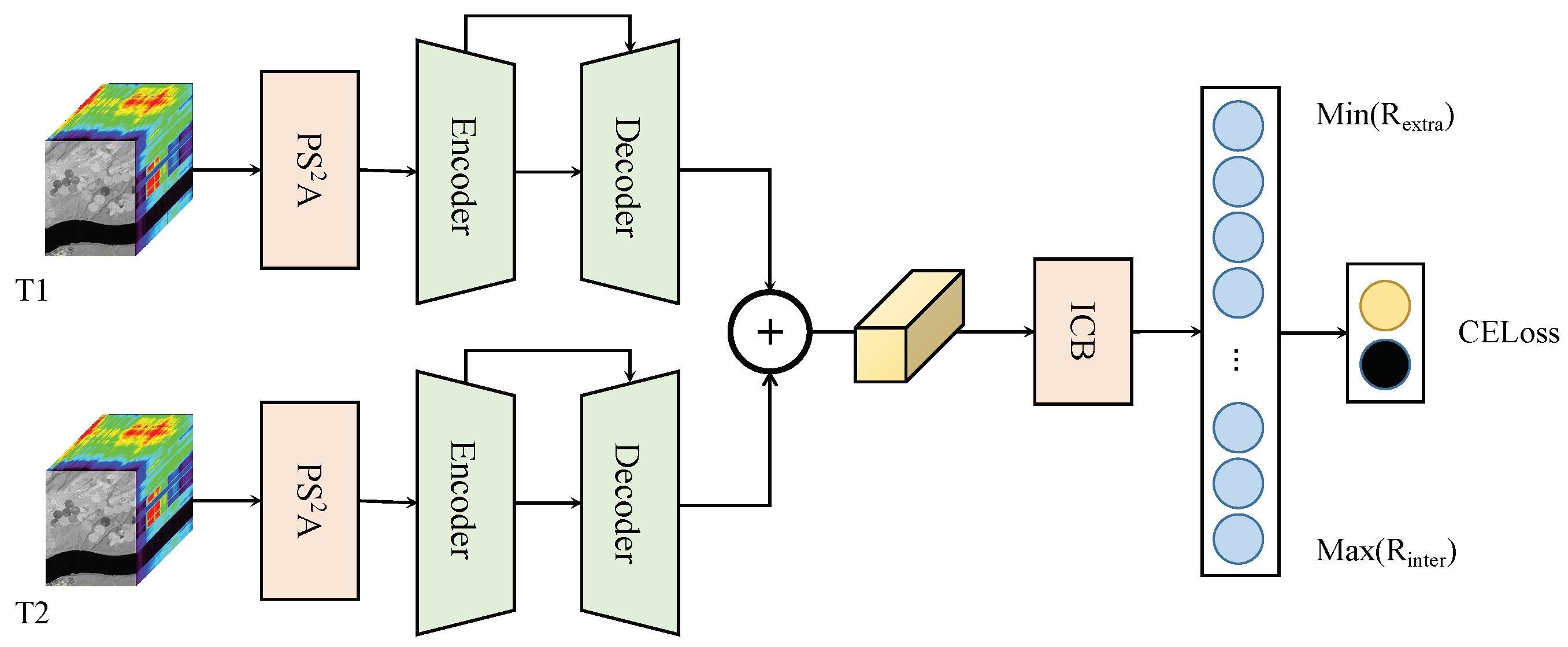
3. Proposed Method

To address these problems and challenges mentioned above and strengthen the robustness and accuracy of model performance, a two-branch feature redistribution network based on the parallel spectral–spatial attention mechanism (TFR-PS${}^2$ANet) is proposed. The overall architecture and module designation are shown in Figure 1.

The hyperspectral image dataset for change detection contains dual-temporal images, which can be described as T1 and T2. First, two parallel spectral–spatial attention modules (${\mathrm{PS}}^2\mathrm{A}$) are inserted at the start of the whole model to obtain long-range dependencies from both the spectral and spatial domain. Second, weighted feature maps are input into the encoder–decoder framework for a further fused and transformed feature representation. Finally, an intensive connection block is applied to distribute the features into the redistribution loss function and the classification loss function to have a better training procedure.

In this section, the proposed method is presented in four parts to give the detailed information of the design of each, which are the parallel spectral–spatial attention module, the two-branch encoder–decoder framework, the intensive connection block, and the feature redistribution loss function.

3.1. Parallel Spectral–Spatial Attention Module

The parallel spectral–spatial attention module (${\mathrm{PS}}^2\mathrm{A}$) is inserted in the first stage to aggregate the long-range dependencies from the original hyperspectral images as much as possible. As the module name implies, ${\mathrm{PS}}^2\mathrm{A}$ is composed of spectral attention and spatial attention, but each attention map is computed in parallel. The design details of the proposed ${\mathrm{PS}}^2\mathrm{A}$ module are shown in Figure 2.

For a hyperspectral image input patch ${\mathit{x}}_{ori}$ in the shape of ${\mathbf{R}}^{H\times W\times D}$, the parallel spectral and spatial attention module is introduced. Regarding the processing of the spectral attention mechanism, the query vector is defined as ${\mathit{v}}_q^{spec}$, which is used as a reassignment factor for the attention map along with the key vector ${\mathit{v}}_k^{spec}$. A convolutional layer with a $1\times 1$ kernel size is introduced to decrease the spectral channel of the input patch ${\mathit{x}}_{ori}$, followed by two adjacent fully connected layers with the SoftMax activation function to make the query vector ${\mathit{v}}_q^{spec}$ eventually. In reference to the key vector ${\mathit{v}}_k^{spec}$, it is computed by a convolutional layer with 2 dilation rates, which can expand receptive field, followed by a reshape operation to change the features into a size of ${\mathbf{R}}^{HW\times D/2}$. After ${\mathit{v}}_q^{spec}$ and ${\mathit{v}}_k^{spec}$ are generated, the matrix multiplication operation ⊗ is inserted between them to obtain the attention map ${\mathit{v}}_{qk}^{spec}$ along with a fully connected layer and a SoftMax activation. All the process steps of the spectral attention module can be formulated as follows:

$${\mathit{v}}_q^{spec}=F_{softmax}\left(F_{fc}^2\left(F_R\left(F_{conv}^{1\times 1}\left(x_{ori}\right)\right)\right)\right)\in {\mathbf{R}}^{1\times HW},$$

(1)

$${\mathit{v}}_k^{spec}=F_R\left(F_{dilation}^{3\times 3}\left(x_{ori}\right)\right)\in {\mathbf{R}}^{HW\times D/2},$$

(2)

$${\mathit{v}}_{qk}^{spec}=F_{softmax}\left(F_{fc}({\mathit{v}}_q^{spec}\otimes {\mathit{v}}_k^{spec})\right)\in {\mathbf{R}}^{1\times D},$$

(3)

where $F_{conv}^{1\times 1}(·)$ denotes the convolution operation with a kernel size of 1 × 1 and $F_{fc}(·)$ denotes the fully connected layer used to squeeze and expand the middle hidden features. The SoftMax activation function is represented as $F_{softmax}(·)$. The dilation convolution operation with a kernel size of $3\times 3$ is formulated as $F_{dilation}^{3\times 3}(·)$, and the reshape operation $F_R(·)$ is applied in the computation of ${\mathit{v}}_q^{spec}$ and ${\mathit{v}}_k^{spec}$. Then, the spectral attention map can be obtained by the matrix multiplication operation ⊗ to have ${\mathit{v}}_v$ weighted, which is also ${\mathit{x}}_{ori}$ here.

With reference to spatial feature extraction, it has a similar process as for spectral feature extraction. The query vector of the spatial domain ${\mathit{v}}_q^{spa}$ is calculated by a convolutional layer with a kernel size of $3\times 3$, followed by an adaptive average pooling operation to compress the spatial size to $1\times 1$ pixels. Then, the fully connected layer and the SoftMax activation function are applied to halve the number of features. As for the vector of spatial key vector ${\mathit{v}}_k^{spa}$, it is calculated by dilation convolution with a kernel size of $3\times 3$ and a dilation rate of 2, followed by the reshape operation to change the feature map size to ${\mathbf{R}}^{D/2\times HW}$. Then, the same matrix multiplication operation ⊗ is applied between ${\mathit{v}}_q^{spa}$ and ${\mathit{v}}_k^{spa}$, followed by the fully connected layer and SoftMax activation function. For the spatial weighting process, the attention map ${\mathit{v}}_{qk}^{spa}$ is reshaped to the same resolution size of ${\mathbf{R}}^{H\times W}$. The detailed calculations are formulated as follows:

$${\mathit{v}}_q^{spa}=F_{softmax}\left(F_{fc}\left(F_{AAP}\left(F_{conv}^{3\times 3}\left(x_{ori}\right)\right)\right)\right)\in {\mathbf{R}}^{1\times D/2},$$

(4)

$${\mathit{v}}_k^{spa}=F_R\left(F_{dilation}^{3\times 3}\left(x_{ori}\right)\right)\in {\mathbf{R}}^{D/2\times HW},$$

(5)

$${\mathit{v}}_{qk}^{spa}=F_R\left(F_{softmax}\left(F_{fc}(v_q^{spa}\otimes v_k^{spa})\right)\right)\in {\mathbf{R}}^{H\times W},$$

(6)

With the obtained attention maps of ${\mathit{v}}_{qk}^{spec}$ and ${\mathit{v}}_{qk}^{spa}$ by Equations (3) and (6), the value vector ${\mathit{v}}_v$ can be parallelly weighted to achieve the spectral and spatial dependency modeling. The local patch-level perception for hyperspectral images can be defined as:

$${\mathit{x}}_{out}^{att}={\mathit{v}}_{qk}^{spa}\odot {\mathit{v}}_v\odot {\mathit{v}}_{qk}^{spec}\in {\mathbf{R}}^{H\times W\times D},$$

(7)

where ⊙ indicates pointwise production for every band and pixel and ${\mathit{v}}_v$ represents the value vector, which here indicates the original patch input ${\mathit{x}}_{ori}$. ${\mathit{x}}_{out}^{att}$ is the output feature map after weighting.

3.2. Two-Branch Encoder–Decoder Framework

Different from the traditional classification backbone following the pyramid structure, here, the proposed feature extractor is guided by the encoder–decoder structure, which is common in the semantic segmentation of natural or biomedical images. Due to the fact that the dual-temporal images may have different local spectral and spatial information at the same pixel location, the feature extractor based on the encoder–decoder framework is constructed and assembled in the proposed method in a parallel manner. The two-branch design of the rectified encoder–decoder feature extractor is shown in Figure 3.

As the left side of Figure 3 shows, the proposed encoder generates internal feature maps using independent convolutional layers with a kernel size of $3\times 3$. The patch size decreases gradually from $9\times 9$ to $1\times 1$. Take the first layer of the encoder network as an example: feature weighted by the attention map in the shape of ${\mathbf{R}}^{9\times 9\times D}$ is input into a convolutional block with three successive convolutional layers, and then, the output feature map $e0\in {\mathbf{R}}^{9\times 9\times 256}$ is calculated and temporarily saved. By a max pooling layer with a kernel size of $2\times 2$, the output features from the last layer are downsampled into the shape of ${\mathbf{R}}^{7\times 7\times 256}$. Therefore, the components of the encoder are made up of the same and stacked convolutions and max pooling operations. As the right side of Figure 3 shows, the decoder is responsible for processing and expanding the output features generated from the encoder components. Take the last output layer in the encoder as an example: the spatial resolution of $e4\in {\mathbf{R}}^{1\times 1\times 16}$ is expanded by the upsampling operation, while the channel number is enlarged by a convolutional layer. The built feature map is defined as $d3\in {\mathbf{R}}^{3\times 3\times 32}$, which has the same shape as the corresponding encoder $e3$. Both $e3$ and $d3$ are concatenated, and hence, the channel dimension is doubled as well. Then, the features are processed by a convolutional block with three successive convolutional layers, which have the same definition as that in the encoder.

Given an input patch ${\mathit{x}}_{en}^i$, a single convolutional layer $F_{CL}(·)$ can be defined as follows, which is constructed with a convolution, a batch normalization, and a SELU activation function:

$$F_{CL}\left({\mathit{x}}_{en}^i\right)=F_{SELU}\left(F_{BN}\left(F_{conv}^{3\times 3}\left({\mathit{x}}_{en}^i\right)\right)\right),i=0,1,\cdots ,4,$$

(8)

In (8), $F_{BN}(·)$ indicates batch normalization and $F_{SELU}(·)$ denotes the SELU activation function. The three successive convolutions are represented as $F_{CL}^3(·)$, and i corresponds to the i-th block of the encoder. Therefore, the relation between the features from the front and back block can be written as follows:

$${\mathit{x}}_{en}^{i+1}=F_{maxpool}\left(F_{CL}^3\left({\mathit{x}}_{en}^i\right)\right),$$

(9)

where $F_{maxpool}(·)$ indicates the max pooling operation used to squeeze the spatial resolution in the encoder part. For the decoder part, the input for every decoder block ${\mathit{x}}_{de}^i$ is processed by the following formula:

$$F_{conv}^{up}\left({\mathit{x}}_{de}^i\right)=F_{ReLU}\left(F_{BN}\left(F_{conv}^{3\times 3}\left(F_{sample}^{up}\left({\mathit{x}}_{de}^i\right)\right)\right)\right),$$

(10)

$${\mathit{x}}_{de}^i=F_{CL}^3\left(F_{concat}(F_{conv}^{up}\left({\mathit{x}}_{de}^{i+1}\right)+{\mathit{x}}_{en}^i)\right),i=0,1,2,3,$$

(11)

The definition of the upsampling with the convolutionis represented in (10), where $F_{sample}^{up}(·)$ indicates the upsampling operation using the nearest interpolation and $F_{ReLU}(·)$ indicates the ReLU activation function. Then, the output features of the upsampling with the convolutionis concatenated along with the corresponding copy ${\mathit{x}}_{en}^i$ from the encoder and computed by sequential convolutional layers $F_{CL}^3(·)$.

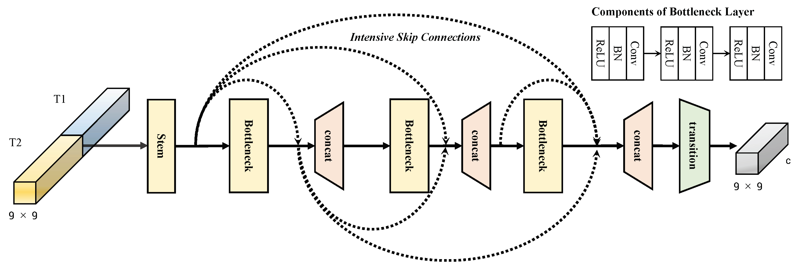
3.3. Intensive Connected Block

To keep the information flow fluent and to pass the hierarchical features, the intensive connected block is constructed. Compared to the residual skip connection, three bottleneck layers with intensive skip connections here were applied to make the model have a low computation cost while keeping a similar time complexity, which was inspired by DenseNet [33].

The input features ${\mathit{x}}_{ICB}^{in}\in {\mathbf{R}}^{H\times W\times 64}$ are concatenated by two output feature sets generated from two-branch encoder–decoder framework. Then, it is processed by the stem layer to reduce the channel number to avoid overfittingin the intensive skip connections. When feature maps arrive at the last skip connection, the channel number is expanded by three bottleneck layers. Therefore, a transition layer is introduced to avoid the burden of too many features. The process in the intensive connected block can be formulated as follows:

$${\mathit{x}}_0=F_{stem}\left({\mathit{x}}_{ICB}^{in}\right)=F_{conv}^{3\times 3}\left({\mathit{x}}_{ICB}^{in}\right)\in {\mathbf{R}}^{H\times W\times 32},$$

(12)

$${\mathit{x}}_l=\mathit{\beta }\left(F_{concat}(x_0+x_1+\cdots x_{l-1})\right),l=1,2,3,$$

(13)

$${\mathit{x}}_{ICB}^{out}=F_{transition}\left(x_3\right)=F_{conv}^{1\times 1}\left(F_{ReLU}\left(F_{BN}\left(x_3\right)\right)\right)\in {\mathbf{R}}^{H\times W\times 16},$$

(14)

where $F_{stem}(·)$ indicates a stem convolutional layer with a $3\times 3$ kernel size to decrease feature channel number and $\mathit{\beta }(·)$ indicates the bottleneck layer shown in Figure 4. $F_{transition}(·)$ denotes the transition layer for the computation of the feature output ${\mathit{x}}_{ICB}^{out}$.

3.4. Feature Redistribution Loss Function

To obtain a better class-oriented feature expression, the feature redistribution loss function (FRL) was developed to distribute the features more properly. The feature redistribution can provide enhanced and fused features for pattern recognition [14]. Inspired by this work and due to the procedure of the conventional loss computation lacking class distribution information for change detection, the FRL is proposed and can enhance the independence of the feature representation. The structure of the FRL is shown in Figure 5.

After the process of the ICB, the output features ${\mathit{x}}_{ICB}^{out}$ are convoluted to ${\mathit{x}}_{FRL}^{in}\in {\mathbf{R}}^{9\times 9\times 16}$, followed by a fully connected layer to change the features to ${\mathit{x}}_G\in {\mathbf{R}}^{1\times 1\times 64}$. Then, the features ${\mathit{x}}_G$ are divided into a set of vectors of length m. Therefore, the defined feature number of vectors is calculated as:

$$n=64/m.$$

(15)

The number of divided groups is the same as the number of land cover change categories c, and the covariance matrix $\mathit{C}$ corresponding to the variants n can be calculated as:

$$\mathit{C}=\frac{1}{m}\sum _{i=1}^m({\mathit{x}}_i-\mu ){({\mathit{x}}_i-\mu )}^T\in {\mathbf{R}}^{n\times n},$$

(16)

$$\mu =\frac{1}{m}\sum _{i=1}^m{\mathit{x}}_i,$$

(17)

where $\mu \in {\mathbf{R}}^{n\times 1}$ indicates the mean vector of vector length m. All defined n features can be represented as V and grouped into c categories $\{G_1,G_2,\cdots ,G_c\}$. Every group contains $s=n/c$ defined features. With the constructed covariance matrix $\mathit{C}$, the correlation matrix can be represented as $\mathit{Re}$, where the correlation coefficient between the indices of i and j is calculated as:

$${\mathit{Re}}_{ij}=\frac{|{\mathit{C}}_{ij}|}{\sqrt{{\mathit{C}}_{ii}{\mathit{C}}_{jj}}},$$

(18)

To maximize the correlation between extra-groups ${\gamma }_{extra}$ and minimize the correlation in inter-groups ${\gamma }_{inter}$, both correlations can be defined as follows:

$${\gamma }_{extra}=\sum _{k=1}^c\frac{{\sum }_{i\in G_k,j\in V-G_k}{\mathit{Re}}_{ij}}{{\sum }_{i\in G_k,j\in V}{\mathit{Re}}_{ij}},$$

(19)

$${\gamma }_{inter}=\sum _{k=1}^c\frac{{\sum }_{i,j\in G_k}{\mathit{Re}}_{ij}}{{\sum }_{i\in G_k,j\in V}{\mathit{Re}}_{ij}},$$

(20)

Considering a simple and convenient representation of the formula in (19), the part that represents the correlation for the k-th group can be defined as:

$${\mu }_k=\frac{{\sum }_{i\in G_k,j\in V-G_k}{\mathit{Re}}_{ij}}{{\sum }_{i\in G_k,j\in V}{\mathit{Re}}_{ij}},$$

(21)

According to the correlation matrix $\mathit{Re}$ and the relation of the indices in ${\mu }_k$, the interval of ${\mu }_k$ can be calculated and ${\gamma }_{extra}$ can be simplified as well:

$${\mu }_k\in [0,\frac{c-1}{c}],$$

(22)

$${\gamma }_{extra}=\sum _{k=1}^c{\mu }_k,$$

(23)

Therefore, the normalized loss between the extra-groups can be represented as:

$$Los{s}_{extra}=\frac{c}{c(c-1)}\sum _{k=1}^c{\mu }_k\in [0,1],$$

(24)

Maximizing the internal correlation ${\gamma }_{inter}$ is equivalent to minimizing $\frac{1}{{\gamma }_{inter}}$. The definition is as follows:

$${\sigma }_k=\frac{{\sum }_{i\in G_k,j\in V}{\mathit{Re}}_{ij}}{{\sum }_{i,j\in G_k}{\mathit{Re}}_{ij}}\in [1,c],$$

(25)

Therefore, the normalized loss of the internal correlation can be calculated with:

$$Los{s}_{inter}=\frac{1}{c(c-1)}\sum _{k=1}^c{\sigma }_k-1\in [0,1],$$

(26)

With the calculated extra-loss and inter-loss, it can be assembled together by the weights’ distribution. The whole loss function can be represented as below:

$$Loss={\lambda }_2({\lambda }_{1}Los{s}_{extra}+(1-{\lambda }_1)Los{s}_{inter})+(1-{\lambda }_2)CELoss,$$

(27)

where ${\lambda }_1,{\lambda }_2\in (0,1)$ indicate the weight coefficients to adjust the sizeof every loss. $CELoss$ indicates the cross-entropy loss. The effectiveness of the proposed loss function is discussed in the later ablation experiments, and the impacts of the hyperparameters are analyzed as well.

After the redistribution loss is applied, the features are sent to the fully connected layer, followed by SoftMax activation function, which links the cross-entropy loss function. This prediction procedure can be formulated as:

$$y_{pred}=F_{softmax}\left(F_{fc}\left(x_G\right)\right).$$

(28)

4. Experiments

4.1. Description of Dataset

In this paper, three public dual-temporal datasets for hyperspectral change detection were chosen for model testing, which were all captured by the Earth Observing-1 (EO-1) satellite with the Hyperion sensor. It provides a spectral range of 0.4–2.5 μm with 242 spectral bands and a spectral resolution of 10 nm approximately, as well as a spatial resolution of 30 m. In the experiments, spectral bands with a low signal-to-noise ratio (SNR) were removed. To distinguish whether the land cover area had changed or not, the binary ground truth maps were obtained by visually analyzing extensive studies and on-the-spot investigation. The first hyperspectral image dataset is the Irrigated Agriculture Dataset [34] captured on 1 May 2004 and 8 May 2007, which illustrates an irrigated agricultural area of Hermiston City in Umatilla County, Oregon, USA. It contains $307\times 241$ pixels and 156 bands after omitting no-data bands and removing the noise. The training rate followed the original work, which was 9.7% approximately. This dataset is shown in Figure 6. The second dataset is the Wetland Agriculture Dataset [34], which contains images captured on 3 May 2006 and 23 April 2007. This dataset illustrates a farmland area of Yuncheng City, Zhejiang Province, China. It contains $450\times 140$ pixels and 156 bands after removing noise. Referring to the training rate of the Irrigated Agriculture Dataset, the training samples for the Wetland Agriculture Dataset were further decreased compared to the original work, which was set to about 9.7% as well. 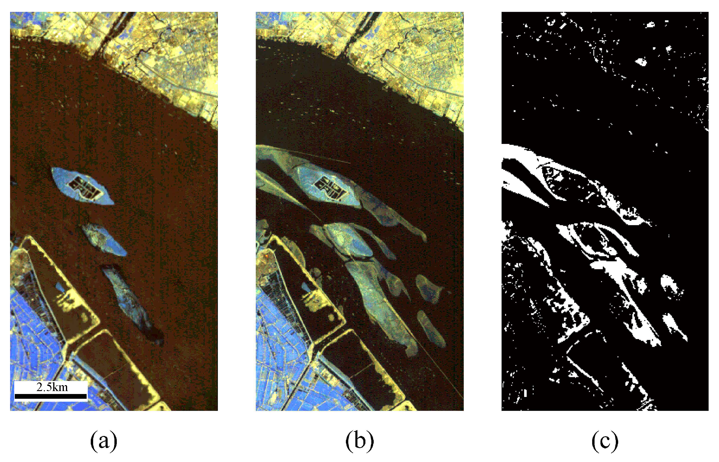The T1 image, T2 image, and ground truth are shown Figure 7. The last change detection dataset is the River Dataset [26], which contains images captured on 3 May 2013 and 31 December 2013. This dataset illustrates a river area in Jiangsu Province, China. It contains $463\times 241$ pixels and 198 bands after noise removal. The false color image for the River Dataset is shown in Figure 8. Every dataset was divided into a training set, validation set, and test set. The training samples of the Irrigated Agriculture Dataset and Wetland Agriculture Dataset occupied 9.7% of the total samples approximately using stratified random sampling. For the River Dataset, to consider the problem of class imbalance, the proportion of the unchanged samples to the changed samples was 2:1, which followed the rule of original work. Eventually, the training rate for the River Dataset was 4.03%. For all three public datasets, stratified random sampling was used to generate the random training samples. The details of every dataset are shown in

Table 1. Details of the selected datasets.

Dataset	Spatial Size	Band	Date 1	Date 2	Training Rate	Training Samples
Irrigated	$307\times 241$	156	May 1st, 2004	May 8th, 2007	9.7%	7250
Wetland	$450\times 140$	156	May 3rd, 2006	Apr. 23rd, 2007	9.7%	6173
River	$463\times 241$	198	May 3rd, 2013	Dec. 31st, 2013	4.03%	4500

.

4.2. Experimental Setup

All experiments were performed on an NVIDIA RTX 3060 with 12G of video memory. Due to the model structure, it can handle different patch input sizes without any spatial resolution restriction. In the training set procedure, the batch size was chosen as 64 patch inputs by default and the learning rate as ${10}^{-5}$ with a corresponding ${10}^{-4}$ weight decay applied to exhibit better convergence. The Adagrad optimizer was used here to train the proposed TFR-PS${}^2$ANet. The united loss function with the cross-entropy loss and the feature redistribution loss were chosen for the model training procedure, and the formula of the cross-entropy loss is shown below:

$$L=\frac{1}{N}\sum _i{L}_i=-\frac{1}{N}\sum _i\sum _{c=1}^M{y}_{ic}log\left(p_{ic}\right),$$

(29)

where M indicates the number of categories and $y_{ic}$ is an indicator for which the value is equal to 1 or 0 depending on whether it is the true category of sample i. The prediction probability belonging to c of sample i is expressed as $p_{ic}$.

4.3. Evaluation Metrics

For a fair and convenient performance comparison among the three hyperspectral change detection datasets, the accuracy (ACC), kappa coefficient (kappa), F1-score, precision, and recall were selected to evaluate and quantized model’s performance. Every index was calculated based on a confusion matrix, and the larger the value, the better the performance is.

Accuracy (ACC): Regarding pixel-level classification tasks, accuracy is a relatively simple, but effective metric to weigh the model’s performance. The formula for the calculation of the accuracy is:

$$ACC=\frac{{\sum }_{i=0}^{c}T{P}_i}{{\sum }_{i=0}^c(T{P}_i+F{P}_i)}.$$

(30)

Kappa coefficient (kappa): The kappa coefficient is another metric usually used for pixel-level classification. According to the formula of the kappa coefficient, it takes the class imbalance into consideration and can measure the model’s performance on different datasets fairly. The formula for the calculation of the kappa coefficient is:

$$k=\frac{p_o-p_e}{1-p_e}.$$

(31)

F1-score: The F1-score (also known as the F1-measure) is designed to evaluate the performance of a pixel-level binary classification model. It can be considered as the harmonic mean of the precision and recall. The F1-score is calculated as:

$$\mathrm{F}1=2·\frac{precision\times recall}{precision+recall}.$$

(32)

Precision and recall: The precision indicates the true positives in the sum of the true positive and false positive samples. The recall indicates the true positives in the sum of the true positive and false negative samples. The formulae are, respectively:

$$Precision=\frac{TP}{TP+FP},$$

(33)

$$Recall=\frac{TP}{TP+FN}.$$

(34)

4.4. Experimental Results

In this section, five methods in the change detection domain were chosen to make comparisons with the proposed TFR-PS${}^2$ANet. Two of them are traditional methods based on supervised or unsupervised learning, and the rest are SOTA deep learning methods. CVA is a traditional method using difference maps and unsupervised segmentation, which was Otsu here [35]. The second traditional method for pattern recognition is SVM, which is extensively used in land cover change detection [36]. As for the deep learning methods, GETNET [26] based on the LSConvolution architecture and DSFANet [27] following the principle of semi-supervised learning were chosen as the comparison methods. 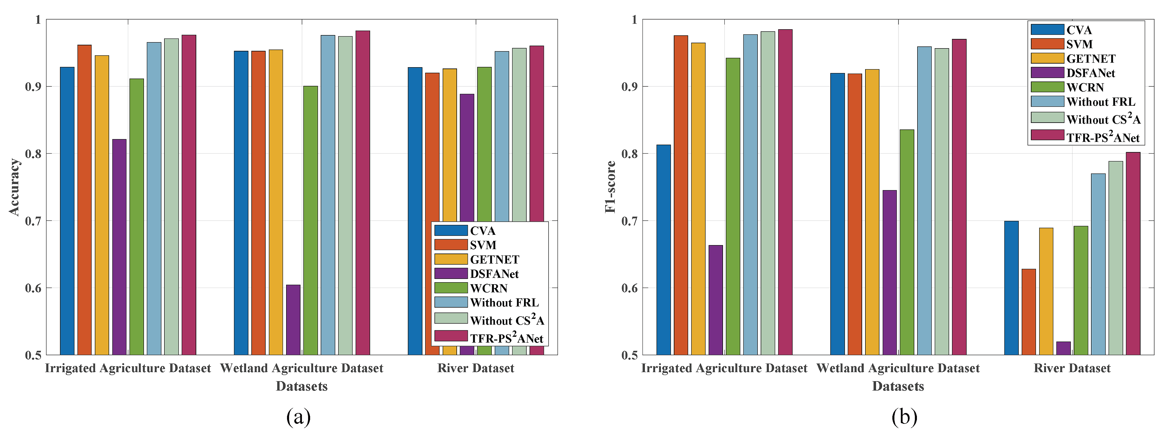For the CNN architecture in two-domain learning, the patch-based WCRN model [19] was chosen as the comparison model. For the mentioned deep-learning-based methods, the same default parameter settings introduced in the corresponding works were selected. Extensive experiments were conducted on all three hyperspectral change detection datasets. The detailed model comparison results are described below. The overall accuracy and F1-score comparison is shown in Figure 9, which indicates that the proposed TFR-PS${}^2$ANet is superior to most of the other methods.

4.4.1. Experiments on the Irrigated Agriculture Dataset

The model comparison results can be seen in

Table 2. Model comparison results and module ablation study results on the Irrigated Agriculture Dataset (repeated 3 times).

Models	ACC	Kappa	F1-Score	Precision	Recall
CVA	0.9286	0.7704	0.8127	0.9953	0.6867
SVM	0.9614 ± 0.0021	0.8868 ± 0.0117	0.9754 ± 0.0008	0.9657 ± 0.0193	0.9854 ± 0.0184
GETNET	0.9456 ± 0.0080	0.8466 ± 0.0172	0.9646 ± 0.0057	0.9690 ± 0.0091	0.9608 ± 0.0203
DSFANet	0.8208 ± 0.0073	0.5449 ± 0.0023	0.6631 ± 0.0154	0.5754 ± 0.0114	0.7823 ± 0.0219
WCRN	0.9113 ± 0.0060	0.7516 ± 0.0164	0.9422 ± 0.0039	0.9509 ± 0.0033	0.9336 ± 0.0045
Without FRL	0.9652 ± 0.0054	0.9039 ± 0.0133	0.9772 ± 0.0037	0.9920 ± 0.0051	0.9629 ± 0.0122
Without ${\mathrm{PS}}^2\mathrm{A}$	0.9709 ± 0.0014	0.9159 ± 0.0050	0.9813 ± 0.0009	0.9765 ± 0.0050	0.9862 ± 0.0033
TFR-PS${}^2$ANet	0.9763 ± 0.0009	0.9324 ± 0.0028	0.9846 ± 0.0005	0.9862 ± 0.0029	0.9831 ± 0.0019

. The proposed TFR-PS${}^2$ANet was able to achieve the best results on the ACC, kappa coefficient, F1-score, and recall. The best precision was achieved by CVA, while this model had the worst recall result, which is less than about 0.29 compared to that of TFR-PS${}^2$ANet. The best competitor was the SVM method. As a traditional method, it outperformed most of the selected deep learning methods. Among them, the unsupervised DSFANet showed the worst change detection results. GETNET showed the best recall in comparison to the other methods, but its precision was lower than that of TFR-PS${}^2$ANet, which resulted in an inferior F1-score result. DSFANet is an unsupervised method just like CVA, but it detects too many unchanged pixels wrongly according to its poor precision performance, which may be a result of the complex scenes of the agriculture images.

In the last three rows of Table 2, the comparisons of TFR-PS${}^2$ANet, TFR-PS${}^2$ANet without redistribution loss, and TFR-PS${}^2$ANet without ${\mathrm{PS}}^2\mathrm{A}$ are given. The accuracy and kappa coefficient performance of TFR-PS${}^2$ANet without redistribution loss showed a clear drop compared to TFR-PS${}^2$ANet. TFR-PS${}^2$ANet without ${\mathrm{PS}}^2\mathrm{A}$ showed a slight accuracy decrease, while the kappa coefficient had an obvious disparity. Although the two ablation studies of the models demonstrated weaker results than TFR-PS${}^2$ANet, they still outperformed the other competitors, which implies that the encoder–decoder framework can effectively extract the change features. In conclusion, the proposed TFR-PS${}^2$ANet had the best performance on most of the metrics compared to the other methods.

The change detection maps for the Irrigated Agriculture Dataset are shown in Figure 10. Using the ground truth map as a reference, the proposed TFR-PS${}^2$ANet showed the closest visual effects, and the border pixels were visually distinct like the ground truth map, while the change maps detected by CVA, GETNET, and WCRN failed to distinguish the subtle changes in the border pixels. Although SVM showed great visual effects, it detected unrelated subtle changes of the border pixels mistakenly, which led to inferior accuracy and precision. Regarding DSFANet, it showed scattered points in the change result map, which caused a false detection and led to lower accuracy and kappa indices. The reason for this situation could be that the unsupervised DSFANet is not suitable for complex land cover spectral information. Regarding the ablation results of the models TFR-PS${}^2$ANet without redistribution loss or ${\mathrm{PS}}^2\mathrm{A}$, it can be seen from the visual effects that TFR-PS${}^2$ANet without redistribution loss would detect some border pixels mistakenly, while TFR-PS${}^2$ANet without ${\mathrm{PS}}^2\mathrm{A}$ would detect border pixels as a large spot, which would affect the detection result.

4.4.2. Experiments on the Wetland Agriculture Dataset

The comparison results of the models on the Wetland Agriculture Dataset are shown in

Table 3. Model comparison results and module ablation study results on the Wetland Agriculture Dataset (repeated 3 times).

Models	ACC	Kappa	F1-Score	Precision	Recall
CVA	0.9525	0.8859	0.9196	0.9032	0.9366
SVM	0.9525 ± 0.0015	0.8851 ± 0.0045	0.9185 ± 0.0035	0.9150 ± 0.0072	0.9223 ± 0.0144
GETNET	0.9543 ± 0.0128	0.8926 ± 0.0274	0.9253 ± 0.0177	0.8926 ± 0.0548	0.9644 ± 0.0255
DSFANet	0.6043 ± 0.0025	−0.1127 ± 0.0060	0.7452 ± 0.0032	0.6861 ± 0.0007	0.8157 ± 0.0088
WCRN	0.9003 ± 0.0362	0.7643 ± 0.0802	0.8355 ± 0.0535	0.8170 ± 0.0354	0.8579 ± 0.0179
Without FRL	0.9760 ± 0.0025	0.9419 ± 0.0063	0.9589 ± 0.0045	0.9538 ± 0.0026	0.9640 ± 0.0119
Without ${\mathrm{PS}}^2\mathrm{A}$	0.9743 ± 0.0044	0.9380 ± 0.0016	0.9561 ± 0.0075	0.9490 ± 0.0075	0.9633 ± 0.0075
TFR-PS${}^2$ANet	0.9827 ± 0.0004	0.9580 ± 0.0008	0.9701 ± 0.0005	0.9754 ± 0.0081	0.9648 ± 0.0072

. For this dataset, the proposed method TFR-PS${}^2$ANet outperformed the other methods in all indices as well. The best competitor was GETNET, which achieved the highest accuracy in comparison the other models, but it was inferior to TFR-PS${}^2$ANet by a slight worse accuracy and kappa coefficient. CVA and SVM were still stable models, achieving very similar accuracy and kappa coefficient performance. DSFANet showed the worst performance and almost could not detect the main farm change region, which can be concluded from the kappa coefficient result. WCRN could achieve an acceptable accuracy result, but the kappa coefficient remained low.

The last three rows of Table 3 show the comparison among TFR-PS${}^2$ANet, TFR-PS${}^2$ANet without redistribution loss, and TFR-PS${}^2$ANet without ${\mathrm{PS}}^2\mathrm{A}$. Compared to TFR-PS${}^2$ANet, the ablation results of the model TFR-PS${}^2$ANet without redistribution loss were inferior on every metric. The performance of TFR-PS${}^2$ANet without ${\mathrm{PS}}^2\mathrm{A}$ was worse than TFR-PS${}^2$ANet without redistribution loss, which may indicate that long-range dependencies are very necessary in areas with much crop spectral information. In conclusion, the proposed TFR-PS${}^2$ANet showed the best performance on the Wetland Agriculture Dataset.

The detected change maps of these methods for the Wetland Agriculture Dataset are shown in Figure 11. The proposed TFR-PS${}^2$ANet showed the most similarity to the ground truth map in visual effects, which kept the detailed change information while suppressing unrelated subtle information. The two traditional methods, CVA and SVM, could detect the main agriculture change area, but too many scattered points were also detected mistakenly, which influenced the accuracy and precision indices. GETNET successfully detected most of the change area, but there was a loss of subtle farmland change information as well. DSFANet showed the worst performance, which basically only detected the border of change areas. This may have resulted from its insufficient capacity to process complex scenes. WCRN could detect most of the change area, but the main drawbacks were that it lost the detailed information and farmland edge change information. Furthermore, in the top area of the WCRN change map, it detected some unrelated points, which decreased the accuracy and precision results. Regarding the last three change maps, it can be observed that they basically had similar visual effects except several wrong pixels detected by mistake, and they all showed the best similarity to the ground truth map compared to the other methods.

4.4.3. Experiments on the River Dataset

The comparison results of different methods on the River Dataset are shown in

Table 4. Model comparison results and module ablation study results on the River Dataset (repeated 3 times).

Models	ACC	Kappa	F1-Score	Precision	Recall
CVA	0.9280	0.6617	0.6992	0.5492	0.9617
SVM	0.9198 ± 0.0008	0.5850 ± 0.0477	0.6278 ± 0.0469	0.5266 ± 0.0092	0.7876 ± 0.0624
GETNET	0.9260 ± 0.0104	0.6508 ± 0.0314	0.6893 ± 0.0267	0.5467 ± 0.0390	0.9368 ± 0.0164
DSFANet	0.8883 ± 0.0067	0.4610 ± 0.0253	0.5196 ± 0.0022	0.4154 ± 0.0212	0.6940 ± 0.0192
WCRN	0.9284 ± 0.0111	0.6544 ± 0.0346	0.6919 ± 0.0295	0.5579 ± 0.0246	0.9158 ± 0.0175
Without FRL	0.9519 ± 0.0019	0.7439 ± 0.0050	0.7699 ± 0.0041	0.6594 ± 0.0310	0.9250 ± 0.0143
Without ${\mathrm{PS}}^2\mathrm{A}$	0.9566 ± 0.0087	0.7649 ± 0.0052	0.7884 ± 0.0037	0.6850 ± 0.0489	0.9286 ± 0.0081
TFR-PS${}^2$ANet	0.9602 ± 0.0003	0.7803 ± 0.0082	0.8019 ± 0.0074	0.7068 ± 0.0038	0.9267 ± 0.0134

. Our proposed TFR-PS${}^2$ANet achieved the best ACC, kappa, F1-score, and precision. WCRN was the best competitor, which was designed in the original work on the River Dataset, and showed the best accuracy performance (0.9284) among the compared deep learning methods, followed by the deep leaning GETNET method, having a 0.9260 accuracy. SVM and DSFANet had a 0.9198 and 0.8883 accuracy, respectively. The unsupervised DSFANet did not perform well, which could be a result of its insufficient feature learning under class imbalance.

In the same way, the last three rows give the ablation results of the models. Compared to TFR-PS${}^2$ANet, the model TFR-PS${}^2$ANet without redistribution loss showed a considerable accuracy drop by around 0.01, while the model without ${\mathrm{PS}}^2\mathrm{A}$ showed a slight accuracy decrease. Therefore, it is necessary for change detection to adopt the class-oriented feature redistribution in the second to last layerfor the River Dataset. In conclusion, the proposed TFR-PS${}^2$ANet can perform best among these methods while handling with class imbalance.

The change detection maps for the River Dataset are shown in Figure 12. It can be observed that TFR-PS${}^2$ANet showed the closest similarity to the ground truth map from the visual effects. The first result map generated by the unsupervised CVA showed many unrelated pixels detectedto the left. On the contrary, the second SVM result map showed a failure to detect change pixels to the left. GETNET, as the best competitor, could detect distinct change areas, but they were expanded slightly. DSFANet showed many points and gaps due to it insufficient unsupervised post-processing. For the visual effects, the change map from WCRN showed rough boundaries, which caused a low-precision result. With reference to the change map generated by TFR-PS${}^2$ANet without redistribution loss or ${\mathrm{PS}}^2\mathrm{A}$, both could detect some noise-like pixels shown ot the top of the change map, which influenced the final accuracy and F1-score, while they still outperformed the other compared methods.

4.4.4. Impact of Hyperparameters

In this section, the influence by both hyperparameters for the redistribution loss and the cross-entropy loss, which are the weights ${\lambda }_1,{\lambda }_2\in [0.2,0.4,0.5,0.6,0.8]$ in Formula (27), were analyzed. The hyperparameter ${\lambda }_1$ is responsible for the adjustment for the extra-loss in the redistribution loss function, while $1-{\lambda }_1$ is responsible for the inter-loss. With the hyperparameter ${\lambda }_1$ selected, the influence of the distribution of the features can be analyzed. The hyperparameter ${\lambda }_2$ was utilized to adjust the influence of redistribution loss, while $1-{\lambda }_2$ worked as the weight for the cross-entropy loss. As Figure 13 shows, the performance impacts for the accuracy, Kappa, and F1-score were analyzed on all three datasets.

The first row shows the accuracy change influenced by hyperparameters ${\lambda }_1$ and ${\lambda }_2$. When ${\lambda }_1=0.2$, the best accuracy performance on the River Dataset was achieved at ${\lambda }_2=0.6$, while that on the Irrigated Agriculture Dataset was achieved at ${\lambda }_2=0.8$. The best accuracy performance on the Wetland Agriculture Dataset was achieved at ${\lambda }_2=0.6$ as well. When ${\lambda }_1=0.4$, the two best accuracies on Wetland Agriculture and River Datasets were both achieved at ${\lambda }_2=0.6$, while on the Irrigated Agriculture Dataset, the proposed method achieved the best performance at ${\lambda }_2=0.5$. Along with the increase of ${\lambda }_1$, the proposed TFR-PS${}^2$ANet could achieve the best accuracy on the three datasets at ${\lambda }_2=0.6$.

The influence on the kappa index is shown in the second row of Figure 13. It had a similar trend to the accuracy change. From the first figure of the second row, it can be observed that the proposed method could achieve the highest kappa results at ${\lambda }_2=0.6$ on the Wetland Agriculture Dataset and the River Dataset, while on the Irrigated Agriculture Dataset, it performed best at ${\lambda }_2=0.8$. When ${\lambda }_1=0.4$, the best results of the kappa index on the Wetland Agriculture and River Datasets were achieved at ${\lambda }_2=0.6$ as well. However, the highest performance on the Irrigated Agriculture Dataset was achieved at ${\lambda }_2=0.5$. According to the last three figures, the proposed TFR-PS${}^2$ANet achieved the highest kappa results when ${\lambda }_2=0.6$ at the same time.

The last row shows the influence on the F1-score index. From the overall visual effects, TFR-PS${}^2$ANet performed stably on both the Irrigated and Wetland Agriculture Datasets. Regarding the analysis of the Irrigated Agriculture Dataset, except the results at ${\lambda }_1=0.2,0.4$, the rest of the figures show that the best F1-score results were achieved at ${\lambda }_2=0.6$ as well. The results on the Wetland Agriculture Dataset showed similar stable trends as those on the Irrigated Agriculture Dataset, which mostly achieved the highest F1-score results at ${\lambda }_2=0.6$. The trends on the River Dataset increased their fluctuation and stopped at ${\lambda }_2=0.6$ to obtain the best performance.

In other words, from the optimal analysis results of the accuracy, kappa coefficient, and F1-score on all three datasets, the proposed model could obtain the best performance when ${\lambda }_1=0.5,0.6,0.8$ and ${\lambda }_2=0.6$. Due to the hyperparameter ${\lambda }_1$ being able to influence the extra- and inter-loss balance, the model hyperparameters were set as ${\lambda }_1=0.5$ and ${\lambda }_2=0.6$ finally.

4.5. Discussion

The advantage in terms of the accuracy of the proposed TFR-PS${}^2$ANet method over the benchmark methods was due mainly to the application of the ${\mathrm{PS}}^2\mathrm{A}$ module, which contains the parallel spectral–spatial attention mechanism. Moreover, the proposed TFR-PS${}^2$ANet method is assisted by the FRL, which can reassign the features to a class-oriented distribution. According to the extensive experiments conducted above, CVA, as the conventional unsupervised method, performed stably on the three datasets. However, the change detection results largely relied on the determination of a threshold. The inadequate extraction of spectral information led to inferior detection results compared to our proposed method. As a conventional supervised method, SVM needs training samples. Practically, it can be difficult for SVM to handle local spatial information while finding a proper discriminative property for spectral information. On the contrary, the proposed method extracts features from both the spectral and spatial domain, which led to better discriminative abilities of change detection.

For the deep learning methods, GETNET is based on the supervised LSConvolution architecture. It extracts features from the input patch without considering internal spectral and spatial dependencies. Our proposed method can adaptively obtain long-range dependencies using the parallel attention mechanism, while the FRL assists in arranging the features properly. DSFANet is performed in a semi-supervised manner. However, this method showed the worst results on all the change detection datasets, which implies its weakness in dealing with complex spectral information using unsupervised post-processing. In terms of the comparison between WCRN and TFR-PS${}^2$ANet, the proposed method using the attention mechanism showed the better effectiveness of the adaptive two-domain feature learning compared to the CNN-based architecture.

However, there are also some limitations of the proposed method. First, the three change detection datasets have different time intervals. This leads to the problem of the continuous change amount during different periods being hard to compare. The design of the proposed method regarding the dual-temporal images as a pair of independent moments indicates that the change monitoring needs the support of data with the same or higher time resolution. To address this issue, it is worthwhile to extend the current TFR-PS${}^2$ANet to time series analysis. Nevertheless, in most situations, a time series change detection method can only be driven by dual-temporal images from satellites with different spectral and spatial resolutions. Therefore, reliable change monitoring results would largely depend on the accurate match between image pairs with different spatial and spectral resolutions. Furthermore, anthropogenic effects may influence the agriculture change results. However, the proposed supervised method based on the binary change ground truth detects changes in the agricultural area without distinguishing whether these changes are caused by human activities. The performance of the supervised change method is largely influenced by the available ground reference labels. Therefore, to detect changes from one labelto another using the change method, more attention should be paid to constructing multiple change ground truths with more informative on-the-spot investigation.

5. Conclusions

In this article, a general network named TFR-PS${}^2$ANet was proposed to detect land cover changes in dual-temporal hyperspectral images. First, the proposed method, which integrates the $\mathrm{P}{\mathrm{S}}^2\mathrm{A}$ module, adaptively extracts spectral and spatial features from input patch pairs. The extracted features enhance the relevant long-range dependencies and suppress the irrelevant information in both the spectral and spatial domain simultaneously. Second, the FRL was added to reassign hidden features to a class-oriented distribution, which can enhance the discriminative ability for changed and unchanged pixels. Moreover, a general two-branch encoder–decoder framework was designed to transform and fuse the high-dimensional information to another characteristic space while keeping the hierarchically transferred features.

We implemented our algorithm and performed experiments on three public hyperspectral change detection datasets. The visual and quantitative results both showed that the proposed method outperformed most of the state-of-the-art methods including conventional and deep network algorithms.

When dealing with different change detection tasks, the proposed TFR-PS${}^2$ANet can be seen as a benchmark method with an adaptive one-stage spectral–spatial feature extraction module. The FRL can provide a reference for various loss functions that accelerate the convergence of the network, as well. In the future, using representation information in self-supervised learning will be considered to improve the performance.