Article

The Influence of Image Degradation on Hyperspectral Image Classification

1
College of Electrical and Information Engineering, Hunan University, Changsha 410082, China
2
Key Laboratory of Visual Perception and Artificial Intelligence of Hunan Province, Changsha 410082, China
3
Institute of Remote Sensing Satellite, China Academy of Space Technology (CAST), Beijing 100101, China
*
Author to whom correspondence should be addressed.
Remote Sens. 2022, 14(20), 5199; https://doi.org/10.3390/rs14205199
Submission received: 1 September 2022 / Revised: 3 October 2022 / Accepted: 10 October 2022 / Published: 17 October 2022
(This article belongs to the Special Issue Advances in Hyperspectral Remote Sensing Image Processing)

Abstract

:
Recent advances in hyperspectral remote sensing techniques, especially in the hyperspectral image classification techniques, have provided efficient support for recognizing and analyzing ground objects. To date, most of the existing classification techniques have been designed for ideal hyperspectral images and have verified their effectiveness on high-quality hyperspectral image datasets. However, in real applications, available hyperspectral images often contain varying degrees of image degradation. Whether or not the classification accuracy will be reduced due to degradation problems in input data, and how it will be reduced become interesting questions. In this paper, we explore the effects of degraded inputs in hyperspectral image classification including the five typical degradation problems of low spatial resolution, Gaussian noise, stripe noise, fog, and shadow. Seven representative classification methods are chosen from different categories of classification methods and applied to analyze the specific influences of image degradation problems. Experiments are carried out from the aspects of single-type synthetic image degradation and mixed-type real image degradation. Consistent results from synthetic and real-data experiments show that the effects of degraded hyperspectral data in classification are related to image features, degradation types, degradation degrees, and the characteristics of classification methods. This provides constructive information for method selection in real applications where high-quality hyperspectral data are difficult to obtain and encourages researchers to develop more stable and effective classification methods for degraded hyperspectral images.

1. Introduction

Hyperspectral image (HSI) classification is a fundamental and important problem in remote sensing image recognition, which is widely used in agricultural production, forestry protection, mineral exploration, urban and rural planning, and land management. To date, HSI classification for different application purposes has been studied for a long time and its performance has been substantially improved. Excellent classification results can be found on high-quality datasets such as the open-access Pavia University, Salinas, and Cuprite datasets. However, in real classification application scenarios, HSIs often suffer from a variety of degradation [1] due to poor imaging devices, natural spectrum variations, atmospheric effects, or bad weather [2,3]. For example, images acquired in bad weather conditions usually contain different levels of shadow and fog, while images taken by facilities with limited imaging conditions may suffer from low spatial resolution and different kinds of noise. Some examples of real degraded HSIs are shown in Figure 1. Whether the excellent classification performance obtained on high-quality HSIs can be maintained on these degraded images is still an open problem worth exploring. As there lacks comprehensive knowledge of the effects of image degradation on HSI classification, we carried out a comparative analysis to fill this gap.
In this paper, we explore this problem by constructing datasets of various degraded images, and quantitatively evaluate and compare the performance of HSI classification methods on synthetic datasets. More specifically, we consider five typical degradations: low spatial resolution, Gaussian noise, stripe noise, fog, and shadow, and synthesize a series of degraded images with a single-type image degradation in different degrees according to their corresponding physical models on four HSI data with different ground objects. Furthermore, we also prepare real HSI data with mixed-type image degradation to enrich our experiments and pursue more reliable results. We choose widely used HSI classification methods covering the existing mainstream classification algorithms and implement them on the entire degraded images. The purpose of this paper is to study the effects of different types and degrees of image degradation on HSI classification compared with ideal high-quality images. The analysis results can help attract more interests in HSI classification of degraded data and provide guidance for further research studies, including the proper selection from massive HSI data and the adaptive construction of HSI classification methods in complex applications. The contributions of the research can be summarized as follows.
  • Five common degradations in HSIs are outlined and modeled by reliable mathematical or physical knowledge. These well-established or refined degradation models can be used to generate simulated hyperspectral images with different types and degrees of degradation, which can be utilized as supplementary data for evaluating the robustness of classification methods or developing new classification methods.
  • A huge volume of HSI data containing single-type and mixed-type degradations are produced and presented. The degraded HSI data with five individual degradation types are constructed from four HSI data in different scenes, while the degraded data with mixed-type degradation are real data which show the situation in a real imaging scene.
  • Comparative experimental results of typical HSI classification methods on the degraded HSI data are given. The effects of five image degradation on HSI classification are analyzed separately. Supplementary experiments on real degraded HSI with mixed-type degradation are also conducted and analyzed. In addition, according to the analysis and discussion, suggestions are provided for both selections of proper images and methods in complex classification applications.
The remainder of the manuscript is organized as follows. In Section 2, we briefly overview the related work of HSI classification and HSI degradation. Section 3 mainly introduces the proposed analysis framework, including the preparation of the degraded HSI data, training and testing methods, evaluation indices, and experimental settings. In Section 4, experimental results are shown and the effects of degraded HSI data in classification are analyzed in the order of single-type degradation and mixed-type degradation. Further discussions are provided in Section 5. The last section provides brief conclusions and recommendations on dealing with classification in practical scenarios and developing target classification methods.

2. Related Work

In this section, we briefly introduced the works related to HSI classification and different categories of degraded HSIs including low spatial resolution images, Gaussian noise images, stripe noise images, foggy images, and shadow images.

2.1. HSI Classification

As one of the most popular applications of HSIs, HSI classification [5] has drawn much attention. Hyperspectral imagers collect the reflection information of the ground surface in hundreds of narrow spectral bands, so HSIs usually contain rich spectral information, which is of great benefit to various applications (e.g., minerals, ocean exploration, precision agriculture, and natural disaster monitoring). Compared with methods of unsupervised classification, supervised classification methods have been studied and applied more widely and frequently since they show higher robustness and accuracy after sample training. From the perspective of the information involved, the existing supervised HSI classification methods can be roughly divided into two groups, namely, the spectral-based methods and the spectral–spatial-based methods [6].
In the early research of hyperspectral image classification, most supervised HSI classification methods focused on employing the high-dimensional spectral information of pixels to determine their class attributes. As a result, many spectral-based pixelwise HSI classification methods emerged, including support vector machines (SVMs) [7], neural networks [8], random forest (RF) [9], and so on. However, due to the large number of features of hyperspectral data and its redundant information between bands, the calculation cost of hyperspectral data classification is very high. To accelerate the computational efficiency, some effective dimension-reduction methods were proposed, e.g., linear discriminant analysis (LDA) [10,11], multinomial logistic regression (MLR) [12], principal component analysis (PCA) [13], and independent component analysis (ICA) [14]. However, the effects from Hughes’ phenomenon [15] and spectral variability [16] are still non-negligible, which limits the performance of those classification methods relying only on spectral information. Therefore, researchers began to consider the spatial information of HSIs when designing classification algorithms.
Generally speaking, in terms of the stage at which spatial information is introduced and works in the classification process, the spectral–spatial HSI classification methods can be separated into preprocessing-based methods, postprocessing-based methods, and hybrid methods [16]. In preprocessing-based methods, the spatial information or/and spectral information are first extracted as feature vectors and then put into the classifier. Obviously, feature extraction and representation are keys to determining the performance of these kinds of methods [17]. For instance, refs. [18,19] extracted the spatial information from adjacent regions and built a sparse representation model where each pixel could be represented by a linear combination of a few bases in the dictionary. In [20,21], the features were generated based on the methods of extended morphological profiles (MPs) and extended morphological attribute profiles (MAPs). Furthermore, the multiple kernel learning [22,23] and superpixel segmentation [24,25] are also widely used methods to extract the spectral–spatial information. In postprocessing methods, the raw classification map is often calculated from a pixelwise HSI classification approach and then optimized according to the spatial dependency [26]. References [27,28] used the Markov random fields (MRF) regularizer to adjust the classification results obtained by the MLR method in dynamic and random subspaces, respectively. In order to optimize the edges of classification results, Kang et al. [29] utilized guidance images on the preliminary class-belonging probability map for edge-preserving. This group of strategies can better describe the boundary of classification objects, remove outliers, and refine classification results. Different from preprocessing-based methods and postprocessing-based methods, spectral and spatial information are used jointly in the whole stage of hybrid classification methods, which means the process of classification is based on the coupling of multiple pieces of information. For example, Li et al. [30] proposed loopy belief propagation (LBP) to estimate the conditional marginals and then introduced them into the active learning (AL) algorithm to improve spectral–spatial hyperspectral image classification. Recently, deep learning methods characterized by a multilayer neural network structure (usually deeper than three layers) have become a growing trend [31], which has also made a great breakthrough in other fields of image recognition [32], natural language processing [33], etc. Compared with traditional HSI classification methods, deep learning models can extract more discriminative features via a series of hierarchically constructed neurons. Networks in different depths focus on depicting different features, in which the shallower layers contain simple features while the deeper layers contain more complicated abstract features. To date, there have been numerous deep learning models proven to be effective in HSI classification. For instance, the stacked autoencoder (SAE) [34] is an integrated network that merges useful high-level features through the combined use of principal component analysis (PCA), deep learning architecture, and logistic regression. Similar to SAEs, the deep belief network (DBN) [35] is also a hybrid framework dependent on the eligibility of a restricted Boltzmann machine (RBM) and DBN. Moreover, the convolutional neural network (CNN) [36] fits various functions through the structures of convolutional layers, pooling layers, and fully connected layers, which makes it possible to train and classify the HSI data after dimension reduction. According to the dimensions of convolution operators, there are 1D CNNs [37], 2D CNNs [38,39], 2D + 1D CNNs [40], and 3D CNNs [41,42].
Although these methods introduced above have made great breakthroughs in HSIs classification, most of them are aimed at high-quality datasets and ignore more common degraded images in real application scenarios. At present, there still lacks the analysis of the impacts of image degradation on HSI classification, hence the purpose of this paper is to bridge this gap.

2.2. HSI Degradation

Due to the limited solar radiation energy received in each band during hyperspectral imaging, it is difficult for hyperspectral sensors to obtain high spatial resolution images similar to multispectral sensors on the same platform, which is more prominent on spaceborne platforms. This problem of low spatial resolution has a certain impact on hyperspectral classification, but the specific impact varies according to the scale of ground objects. When classifying some large-scale ground objects, good classification accuracy can be achieved without relying on high spatial resolution HSIs. On the contrary, when classifying small-scale objects, the HSIs with low spatial resolution are easy to lead to large classification errors. For example, in the hyperspectral image with a 30 m spatial resolution, we can clearly distinguish between water and land, but we cannot distinguish between sporadic houses and roads. For HSIs with low spatial resolution, most of the existing studies improve the spatial resolution of HSIs by the technique of image fusion or super-resolution. Fusing the HSIs with multispectral images (MSIs) or panchromatic images with the higher spatial resolution is a common approach to overcome this problem [43,44]. Dian et al. [45] proposed a method to fuse HSIs with MSIs based on subspace and low tensor multirank regularization, which fully took the spectral correlations and nonlocal similarities into consideration. Lin et al. [46] exploited the advantages of coupled nonnegative matrix factorization (CNMF) and embedded it into the regularization framework to improve the fusion performance. Unlike fusion strategies requiring extra images, the super-resolution can directly reconstruct high spatial resolution images from their original image information [47,48,49]. Mei et al. [50] conducted a super-resolution convolutional neural network to simultaneously improve spatial and spectral resolution. Liu et al. [51] proposed a cascaded end-to-end network via sparse coding to boost the super-resolution performance.
Stripe noise is a category of structural noise caused by inconsistent responses or faulty calibrations of detectors and displayed as a series of stripe patterns in the image. The estimation and removal of stripe noise have been widely considered by many researchers. The methods proposed for stripe removal can be categorized in five groups [52]: methods based on the scene [53,54], methods based on a filter [55], methods based on interpolation [56], methods based on statistics [57,58], and methods based on optimization [59,60]. Liu et al. [61] considered the global sparse distribution and local variational characteristics of stripe noise to build a variational model to achieve stripe separation. Jia et al. [62] destriped HSIs by combining a median linear correction (MLC) and Fourier transform filtering (FTF) based on improved statistics. Yang et al. [63] analyzed the stripe noise properties and proposed a multiscale variation destriping model.
In addition to stripe noise, Gaussian noise is also commonly found in hyperspectral images as the consequence of poor illumination conditions or a high temperature in sensors. This kind of noise is independent of signal information and obeys the Gaussian distribution. As Gaussian noise always coexists with other noise, most of the current research works prefer to deal with the problem of mixed noise in HSIs rather than only considering Gaussian noise. Rasti et al. [64] provided an overview of the noise reduction technique developed in the past decade and discussed the performance of several algorithms. In [65], an automatic noise reduction technique, called HyRes, was proposed based on a sparse low-rank model. In [66], a new denoising method for mixed noise in HSIs was designed by exploiting the low-rank and self-similarity constraints under the assumption of additive noise.
Fog seriously affects the clarity and contrast of HSIs, which confuses the spectral information and harms the subsequent recognition of ground objects. In the field of computer vision, various methods have been designed to restore foggy RGB images, which can be grouped into two categories: methods based on image contrast enhancement and methods based on atmospheric scattering. Methods in the first group aim at optimizing image details to improve image visibility, while methods in the latter group restore the degraded images through establishing and solving the atmospheric scattering model. He et al. [67] proposed a dark channel prior (DCP) model for single-image dehazing, which was a pioneer work in this field. Cai et al. [68] designed an end-to-end system called DehazeNet, which learned and estimated the relationship between hazy image patches and the medium transmission map. In [69], a fog image restoration method was proposed via multiscale image fusion. Based on similar principles, some methods have also been developed and applied to the defogging task of multispectral images. Makarau et al. [70] developed the dark-object subtraction method to acquire the haze density map and presented an automatic process for haze detection and removal in multispectral data. Guo et al. [71] proposed an elliptical boundary prior (EBP) to construct the scattering model for recovering fog-free images. However, there are few studies on defogging methods for HSIs at present, because the priors or constraints used in the existing models are difficult to extend or adjust to HSIs. In [4], a fog model aiming at HSIs was built as a new benchmark and was successfully applied to a large number of fog HSIs captured by satellites.
A shadow, appearing together with clouds, is also a common degradation factor affecting image quality and its following interpretation. For shadow removal in RGB images, sunlight illumination invariance is widely employed as the basis of shadow modeling and compensation correction. Zhang et al. [72] developed a shadow removal system on the basis of illumination recovering optimization. Reference [73] presented a framework to detect the shadow through multiple deep neural networks and constructed a Bayesian formulation model to remove the shadow. As for the research on shadow removal in HSIs, there are broadly two categories of restoration methods: unmixing-based methods and deep-learning-based methods. In [74], the authors exploited the linear unmixing model to estimate the spectral offset for shadow removal, while the restoration of shadow areas in [75] was achieved by nonlinear unmixing. In [76], a feature learning strategy based on a spectral-angle-stacked autoencoder and an illumination model was proposed to recover the shadow areas in HSIs.
Facing these five kinds of image degradation in HSIs, several classification approaches have tried to consider parts of degradation factors in the model design. Liu et al. [77] proposed a method to improve visual recognition under adverse conditions by using robust adverse pretraining algorithms. In [78], dynamic stochastic resonance (DSR) theory was introduced to enhance the shadow areas in HSI classification from both spatial and spectral dimensions. Luo et al. [79] fused the HSIs with light detection and ranging (LiDAR) data to obtain better classification performance in cloud-shadow mixed scenes. Fu et al. [80] proposed a superpixel-based framework that redefined the spectral similarity in the wavelet domain and fused the superpixels with the pixelwise classification results to improve the robustness to random noise. Different from the works mentioned above, this paper focuses on comparisons and analyses of the effects of five types of image degradation problems on HSI classification methods.

3. Proposed Analysis Framework

The proposed analysis framework includes two parts, an experimental setup and the experimental analysis (Figure 2). The first part is to obtain the degraded hyperspectral data with single-type or mixed-type degradation required by the following experiments. The second part aims to realize comparative analyses of the impact of degraded hyperspectral data on classification. In the experiments, more than 7000 classification maps are produced which allow us to compare and analyze the effects of degraded hyperspectral data on classification more objectively. Specifically, the effect analysis mainly includes the effect analysis of single-type degradation and mixed-type degradation.

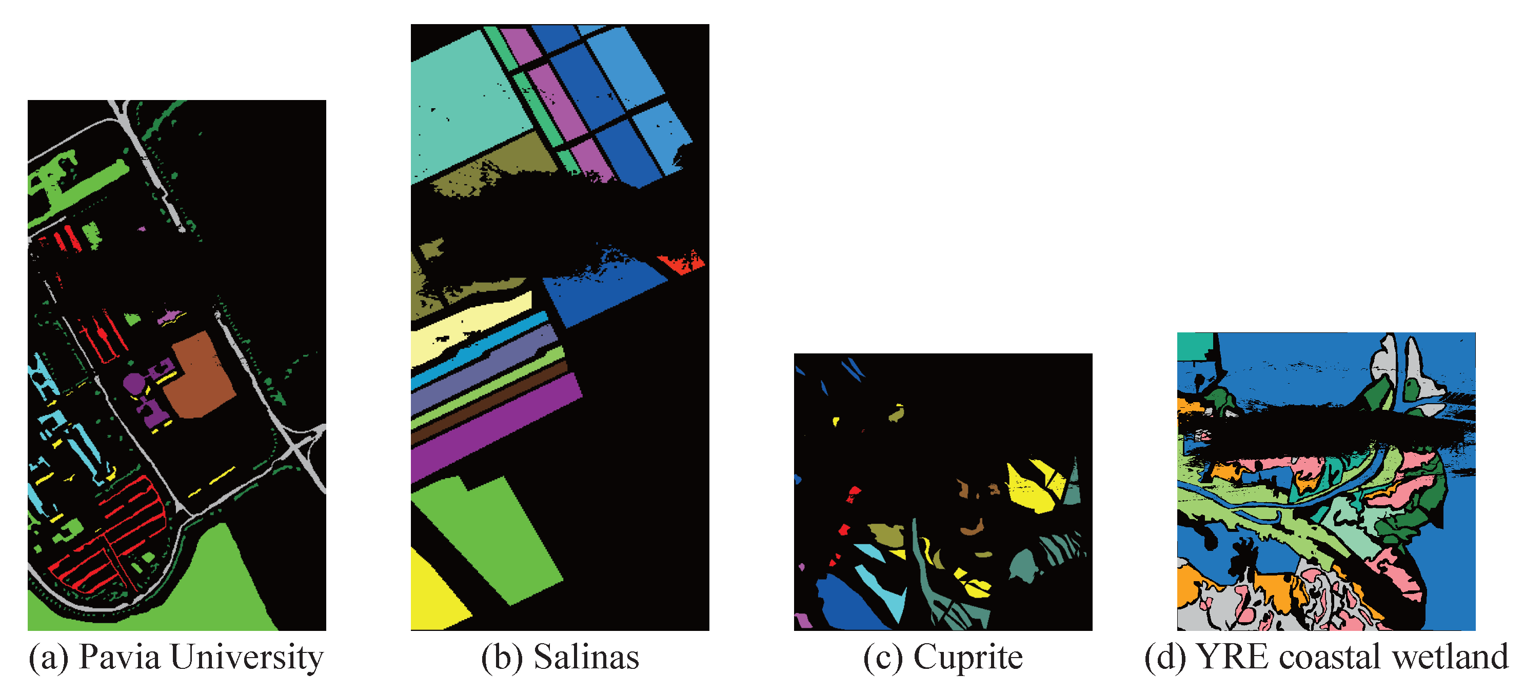
3.1. Data Preparation

In order to carry out experiments more reasonably and comprehensively, we prepared a series of hyperspectral data with single-type and mixed-type degradation. Hyperspectral data with single-type degradation were constructed by a physical-model-based simulation. Four HSI data with different ground objects and spatial resolutions were selected as clean images to realize the syntheses of five kinds of image degradation. They were Pavia University, Salinas, Cuprite, and YRE coastal wetland (see Figure 3).
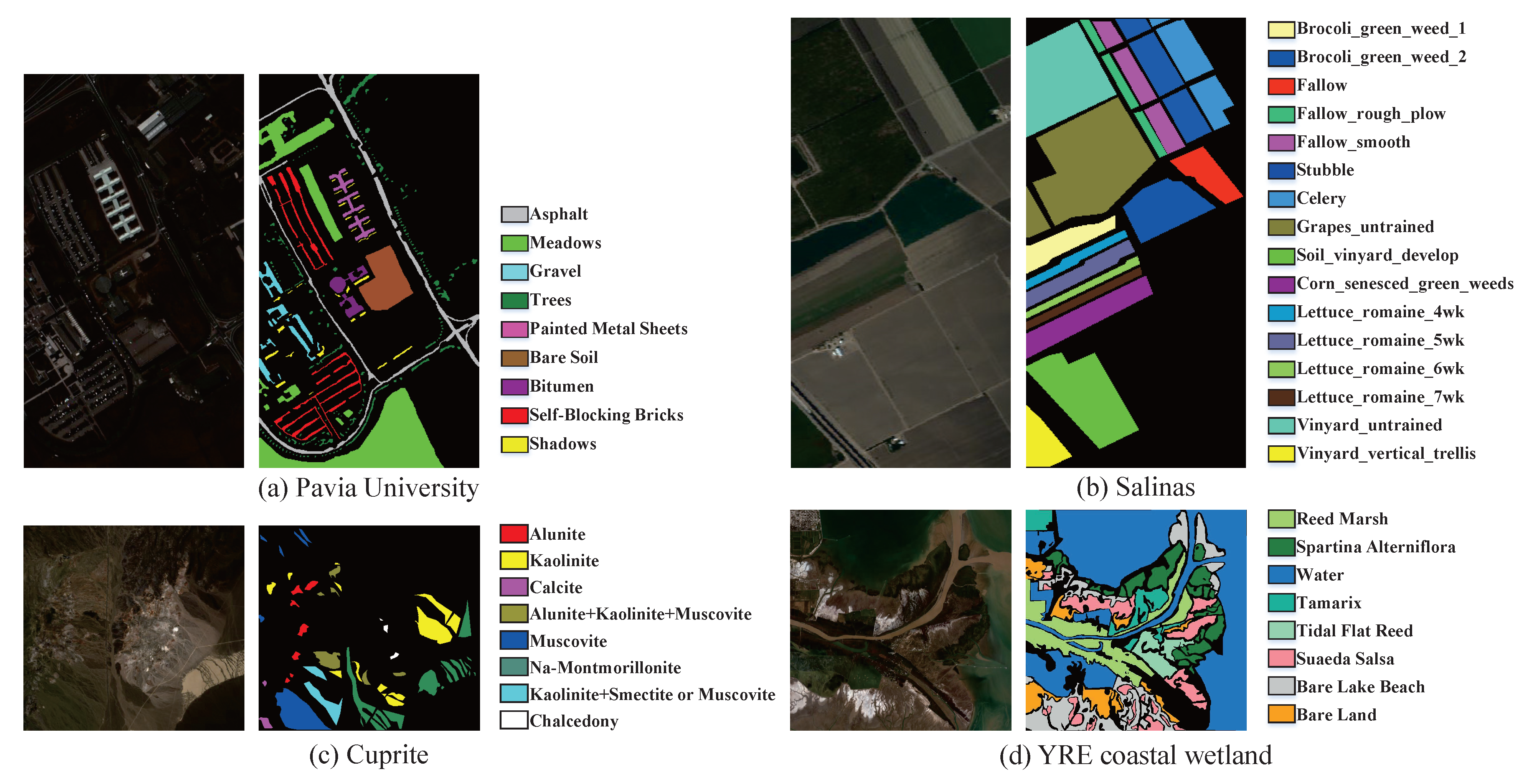
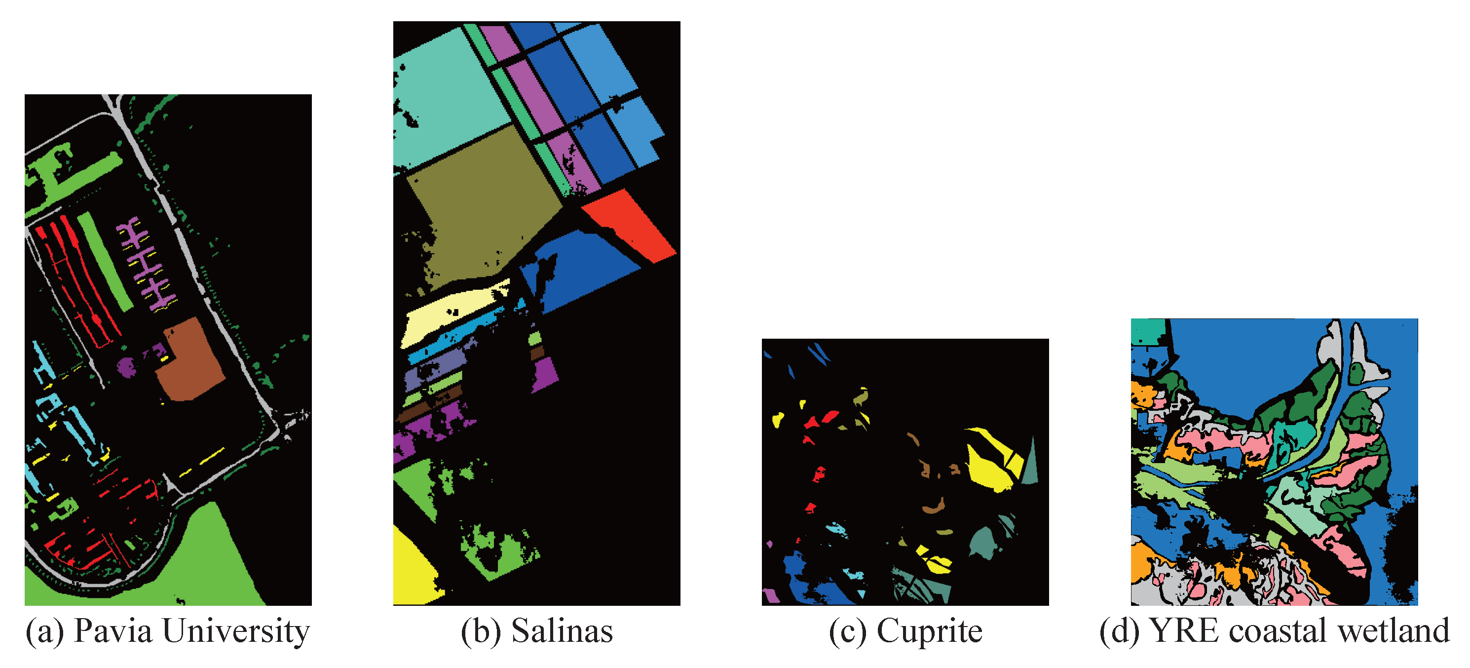
  • Pavia University: It was captured by the reflective optics system imaging spectrometer (ROSIS-3) during a flight over the city of Pavia, northern Italy, in 2003. The image consists of 115 spectral bands within the wavelength range of 0.43–0.86 μ m. Among them, 12 bands were discarded due to noise, and the remaining 103 spectral bands were used in this study. Pavia University contains 610 × 340 pixels with a geometric resolution of 1.3 m. The image is divided into 9 classes in the urban scene, including trees, asphalt roads, bricks, meadows, etc., where 42,776 pixels are labeled;
  • Salinas: This scene was gathered by the Airborne Visible/Infrared Imaging Spectrometer (AVIRIS) sensor over the Salinas Valley in California, USA. Its spatial resolution reaches 3.7 m with 224 spectral bands ranging from 370 nm to 2480 nm. After removing the channels with poor imaging quality (1–2 and 221–224) or related to water absorption (104–113 and 148–167), there remained 188 channels for experiments. The image comprises 512 × 217 pixels, of which 56,975 are background pixels and 54,129 are labeled for classification. Salinas’s ground truth contains 16 categories, including fallow, celery, etc.;
  • Cuprite: Cuprite was also acquired by the AVIRIS sensor, covering cuprite mining areas in Las Vegas, NV, USA. Similar to the Salinas data, there also remained 188 bands after preprocessing. A subimage of 479 × 507 pixels that corresponds to the mineral mapping areas of copper mining reported by the spectral Laboratory of the United States Geological Survey (USGS) [81] was selected for later tests. The ground truth was drawn manually according to the released map (download link: http://speclab.cr.usgs.gov/PAPERS/tetracorder/ (accessed on 1 September 2022)), and was labeled with eight classes, including Alunite, Kaolinite, Calcite, Muscovite, etc. Consistent with the released map, there also exist categories containing two or three kinds of mixed minerals in the manually interpreted ground truth. The total number of labeled pixels is 33,302.
  • Yellow River Estuary coastal wetland (YRE coastal wetland): This data, obtained by the Gaofen-5 satellite, covers the Yellow River Estuary coastal wetland between Bohai Bay and Laizhou Bay, which is the most important representative of the coastal wetland ecosystem in China [82]. The YRE coastal wetland image contains 740 × 761 pixels with 296 spectral bands. The ground sample distance (GSD) of the image is 30 m. According to the records of field observation, the image contains 8 kinds of ground objects, including water, reed, Tamarix, Spartina, etc. There are 415,101 labeled pixels.
Although HSIs are usually subject to a variety of image degradations in real situations, the method of controlled variables was selected to carry out separate simulation experiments on different types of image degradation, so as to better illustrate the effects of degradation types and degradation levels on HSI classification. In our experiment, we set six degradation levels for each degradation type. Figure 4 shows the hyperspectral data with five tested single-type degradation for six degradation levels by taking Cuprite and Salinas as examples.

3.1.1. Hyperspectral Data with Single-Type Degradation

For ease of illustration, the clean HSI is denoted by X R W × H × B , where N = W H is the number of image pixels in the spatial domain, and B is the number of spectral bands. The synthetic degraded HSI is denoted by Y R W × H × B . x i R 1 × 1 × B and y i R 1 × 1 × B stand for the vector at the ith pixel of the hyperspectral image X and Y , respectively.
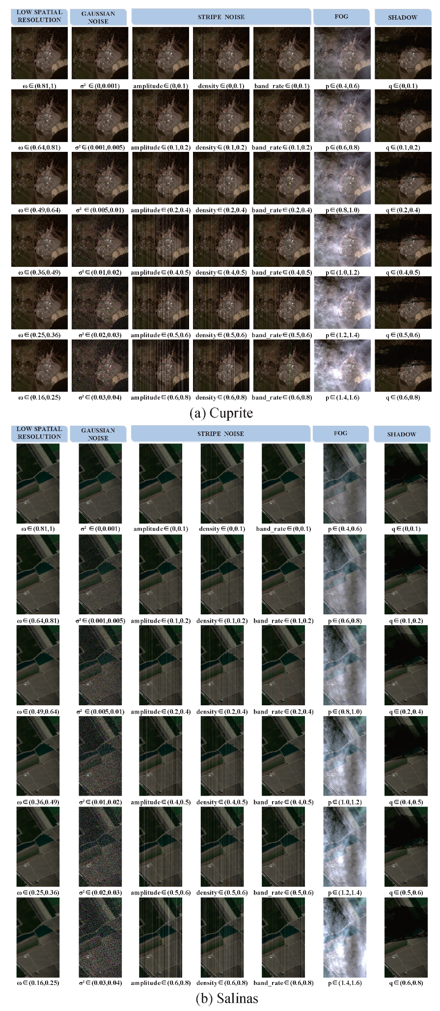
  • Low spatial resolution: To better study the impact of low spatial resolution on image classification, we constructed a series of degraded data with low spatial resolution. The source images were downsampled according to the resolution reduction ratio ω ( ω < 1 ) and then upsampled to the same size as the original images for display. The whole process can be described as:
    Y Low _ resolution = F g 1 / ω F g ω X
    where g denotes the interpolation kernel, F · stands for the sampling function and its two parameters are used to control the sampling process. Given the resolution reduction ratio ω < 1 , F g ω · represents the downsampling process, which transforms the image from R W × H × B to R ω W × ω H × B . Conversely, F g 1 / ω · describes the upsampling process, which transforms the image from R W × H × B to R 1 / ω W × 1 / ω H × B since 1 / ω > 1 . In the subsequent simulation, the bicubic kernel [83] was chosen and the resolution reduction ratio ω was selected as 81%, 64%, 49%, 36%, 25%, and 16%. Clearly, the spatial resolution decreases as ω decreases, and the image becomes more and more blurred in the visual display.
  • Gaussian noise: Gaussian noise is the most common kind of noise, which is caused by random interference in the process of image capture, transmission, or processing. Since Gaussian noise can be regarded as additive noise, we simulated Gaussian noise degraded data series as:
    Y Gaussian = X + G
    where G R W × H × B represents the additive Gaussian noise, whose probability density function at each pixel in each band obeys the distribution as the name implies:
    p ( g ) = 1 σ 2 π e ( g μ ) 2 2 σ 2
    where μ , σ 2 are the expectation and variance of the Gaussian distribution, respectively. To simulate different noise levels, the mean value μ was fixed as 0, and the variance σ 2 of Gaussian noise was adjusted to 0.001, 0.005, 0.01, 0.02, 0.03, and 0.04.
  • Stripe noise: Stripe noise is a kind of directional noise, with pixel values brighter or darker than their adjacent normal image rows/columns, which is usually caused by inconsistent responses of imaging detectors due to unevenness, dark current influence, and environmental interference. For different imaging systems, stripe noise can be randomly distributed or periodically distributed in the image. Considering that the push-broom imaging system is used in hyperspectral imaging, only the randomly distributed stripe noise S R W × H × B was simulated in HSIs. The stripe degradation process can be written as:
    Y Stripe = X + S
    When constructing stripe data, three variables are involved. They are the amplitude of the stripe s a , the density of the stripe s d , and the number of affected bands s b in hyperspectral images. The calculation of s m , s w , s b are separately given as follows:
    s a = r a m p l i t u d e × mean ( X ) s d = r d e n s i t y × W s b = r b a n d × B
    where r ( 0 , 1 ) stands for the ratio of the specific variable and the function mean · refers to the three-dimensional mean calculation on the whole hyperspectral data. In the simulation process, the amplitude of the added stripe was a random number obeying the normal distribution with the mean value as s a . The degree of density s d referred to the number of striped columns in one band, and the locations of stripes were distributed randomly. The number of the affected bands of stripe noise was determined by s b . In addition, we added positive stripes to the random half of the striping locations and negative stripes to the other half to simulate the light and dark distribution of stripe noise. The ratio of the three variables was tested at 6 levels: 10%, 20%, 40%, 50%, 60%, and 80%. It should be noted that in the process of stripe simulation, when one variable was considered for adjustment, the ratio of the other two variables was fixed at 30%.
  • Fog: In foggy weather, hyperspectral imaging records the reflected energy of fog and ground objects at the same time, that is, there is a deviation in the spectral information of ground objects. Then, whether the foggy image affects the hyperspectral classification and to what degree has become a problem worthy of study.
    In order to reasonably add fog to a clean hyperspectral image and make it closer to a real situation, we used the model proposed in [4] for fog simulation, in which the foggy hyperspectral image was modeled as the superposition of the clean image and fog image. Specifically, the authors in [4] first calculated a foggy density map by comparing the average values from visible and infrared bands, since the fog had an obvious effect on the visible bands and almost no effect on the infrared bands. Then, based on the foggy density map and reflectance differences between pixels, fog abundances in different spectral bands were estimated. Finally, by solving the fog model, the fog in the degraded image was removed. Contrary to the fog removal process, we added fog to clean hyperspectral images according to the formulation given in (6). The foggy density map and fog abundance were both extracted from real foggy datasets.
    y Fog i = x i + f i A
    where y Fog i R 1 × 1 × B represents the vector at the ith pixel in the simulated image Y Fog . x i R 1 × 1 × B represents the vector at the ith pixel in the original clean image X . A R 1 × 1 × B stands for the fog abundance estimated from the real foggy HSI. F R W × H × 1 denotes the fog intensity map, and f i represents its ith pixel. In order to evaluate the effects of different fog degradation levels, we simulated the data as follows:
    Y Fog = X + p A F
    where p stands for the fog degradation levels and ⊗ represents the Kronecker product. To be specific, we adjusted the value of p to 0.6, 0.8, 1.0, 1.2, 1.4, and 1.6.
  • Shadow: Shadows in the image represent a significant brightness loss of the ground surface radiation recorded by imagers. Here, we only discuss a shadow caused by inadequate lighting when the sun is blocked, regardless of the shadow caused by tall buildings when the angle of sunlight changes considering that the spatial resolution of hyperspectral images is usually not high enough to generate a large area of building shadows. Since there are few physical models of shadow in hyperspectral images in the current literature, we extended the shadow model of natural images given in [72] to realize a hyperspectral shadow simulation.
    The model proposed in [72] is based on the image formation equation that an observed image is the pixelwise product of the reflectance and illumination [84]. By denoting L i R 1 × 1 × B and R i R 1 × 1 × B as vectors of the illumination L R W × H × B and reflectance R R W × H × B at the ith pixel, the value of x i then satisfies the following formula: x i = L i R i , where ∘ represents the elementwise product. At the same time, the illumination can be described as the sum of direct illumination L i d (illumination generated by the main light source) and ambient illumination L i a (illumination generated by the surrounding environment), i.e., L i = L i d + L i a . Therefore, for each pixel in the shadow area, its ambient illumination intensity can be regarded as unchanged, but the direct illumination intensity reduces significantly. To effectively separate shadows from shadow-affected areas, the corresponding relationship between shadow pixels and intact pixels is established based on texture similarity. The whole model is shown as:
    L i d = s L i a x i = ( L i d + L i a ) R i y Shadow i = ( α i L i d + L i a ) R i α = arg min α T Q α + λ ( α T b S T ) D S ( α b S )
    where s R W × H × 1 denotes an optimized illumination restoration operator, and s i represents its ith pixel. y Shadow i R 1 × 1 × B represents the vector at the ith pixel in the simulated image Y Shadow . α R W H × 1 × 1 is vectorized and describes the degree to which shadows reduce illumination. α can be computed by minimizing the energy equation in the closed-form matting method [85], and α i represents the ith pixel in α . In the energy equation, Q is the Laplacian matrix, D S is a diagonal matrix whose diagonal elements are 1 for constrained pixels and 0 for other pixels, and b S is a vector which records the specified α i values for constrained pixels and 0 for other pixels.
    When extending the model (8) to hyperspectral images, we firstly used a real shadow hyperspectral image caused by a single light source occlusion to extract the optimized illumination restoration operator s and then estimated α by following [85]. The calculation of s is given in (9). Finally, we added the shadow to the clean image according to the operation displayed as:
    s i = x i y i y i α i x i
    y Shadow i = q α i s i + 1 s i + 1 x i
    where q represents the shadow degradation levels, which were set as 0.1, 0.2, 0.4, 0.5, 0.6, and 0.8.

3.1.2. Hyperspectral Data with Mixed-Type Degradation

As for the hyperspectral data of mixed-type degradation, we selected a real degraded HSI called the Chaohu data. The Chaohu data were captured by the Zhuhai-1 satellite, which covered the areas around Chaohu Lake in Anhui, China. These data contain 5865 × 5010 pixels with a geometric resolution of 10 m. There are 32 bands that can be downloaded. As shown in Figure 5a, there is a mixed-type image degradation in the Chaohu data, including Gaussian noise, stripe noise, cloud, and shadow. For the sake of completeness, we labeled the Chaohu data manually referring to the global land cover FROM-GLC10 data (Download link: http://data.ess.tsinghua.edu.cn/fromglc2017v1.html (accessed on 1 September 2022)) and high spatial resolution images from Google Earth. According to the classification system of FROM-GLC10, we interpreted the Chaohu data into six categories, i.e., cropland, forest, grassland, wetland, water, and impervious surface (see Figure 5b). The total number of labeled pixels was 4,670,717.

3.2. Training and Testing Methods

We selected one or two methods from each classification category for comparative experiments. The key concepts of each method are briefly introduced below.
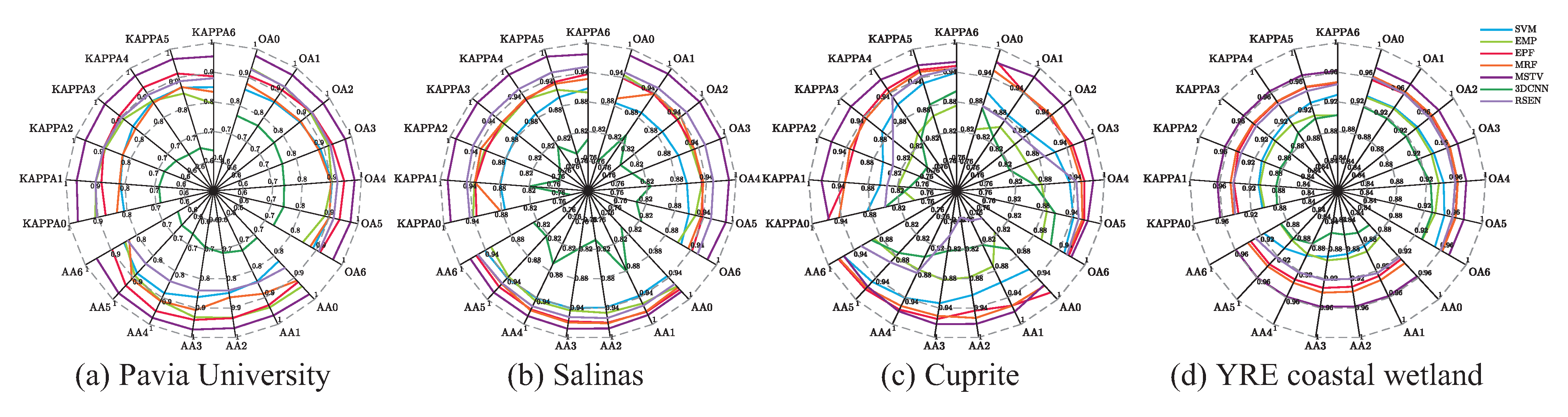
  • Support vector machines (SVMs) [7]: As a spectral-based classification method, the support vector machine (SVM) is one of the most classical and widely used methods whose basic model is the linear classifier with the largest interval defined in the feature space. An SVM was initially designed as a binary linear classification method. However, when the kernel technique is adopted, an SVM can also be used for nonlinear classification in hyperspectral multiclass problems.
  • Extended morphological profiles (EMP) [20]: The extended morphological profiles (EMP) method is a spectral–spatial classification method based on mathematical morphology. The EMP method constructs extended morphological profiles according to the principal components of the hyperspectral data. It mainly considers the spatial information of HSIs and is a preprocessing method, thus generally used together with feature extraction techniques.
  • Edge-preserving filtering (EPF) [29]: Edge-preserving filtering (EPF) is a spectral–spatial classification method based on postprocessing. In this method, the hyperspectral image is first classified by a pixel classifier to obtain a probability map. Then, the probability map is postprocessed by edge-preserving filtering, where the category of each pixel is determined according to the principle of maximum probability. Due to the high computational efficiency, EPF can get considerable classification results at a smaller time cost.
  • Markov random field (MRF) [86]: A Markov random field (MRF) is also a postprocessing spectral–spatial method. Different from EPF, its probability map is optimized through the model of a Markov random field. Specifically, the class of a pixel is determined jointly by the output of the pixelwise classifier, the spatial correlation of adjacent pixels, and the solution of a MRF related minimization problem.
  • Multiscale total variation (MSTV) [87]: Multiscale total variation (MSTV) consists of two steps. The first step is a multiscale structure feature construction where the relative total variation is applied to the dimension-reduced hyperspectral images. Then, multiple principal components are fused by a kernel principal component analysis (KPCA). MSTV can be regarded as a hybrid method since spatial and spectral information is well coupled throughout the classification process.
  • Convolutional neural networks (CNN) [41]: As a data-driven technique, deep learning has been proven to be an effective image classification method due to its accurate semantic interpretation. There are many existing deep learning architectures for remote sensing hyperspectral image classification. Among them, the 3D convolutional neural network can establish a deep comprehension of input images and enables the joint processing of spectral and spatial information for classification. The 3DCNN method was implemented through the source code released in [88].
  • Robust self-ensembling network (RSEN) [89]: The robust self-ensembling network (RSEN) is a recent work that first introduces self-ensembling learning into hyperspectral image classification. An RSEN implements a base network and an ensemble network learning from each other to assist the spectral–spatial network training. A novel consistency filtering strategy was also proposed to enhance the robustness of self-ensembling learning. It is claimed that RSEN can achieve a high accuracy with a small amount of labeled data.
In the comparative experiments, the parameters of each method were consistent with those introduced in the original references, and the code published by the original authors was used. The proportion of training samples was uniformly controlled at 0.5% for different categories in different data. According to the calculation results, the specific numbers of training samples used for different categories in Pavia University, Salinas, Cuprite, and YRE coastal wetland images were set within the range of [ 5 , 94 ] , [ 5 , 57 ] , [ 3 , 45 ] , and [ 62 , 1073 ] , respectively. The numbers of training samples for different categories in the Chaohu data were also set following the same training proportion of 0.5% within the range of [ 63 , 18 , 447 ] . To avoid the interference of accidental factors, each experiment was repeated 10 times and the average accuracy was taken as the final result.

3.3. Evaluation

In order to compare and analyze the effects of degraded hyperspectral data on classification, we applied the aforementioned training and testing methods to the synthetic degraded datasets. The quantitative evaluation was based on three full-reference indices: overall accuracy (OA), average accuracy (AA), and Kappa coefficient. Given S U M denotes the number of labeled samples shown in (11), the numerical definitions of the three indices are written as follows:
S U M = i = 1 n j = 1 n m i j
O A = i = 1 n m i i S U M
A A = 1 n i = 1 n m i i j = 1 n m i j
K a p p a = S U M i = 1 n m i i i = 1 n ( j = 1 n m i j j = 1 n m j i ) ( S U M ) 2 i = 1 n ( j = 1 n m i j j = 1 n m j i i )
where m i j represents the element at the corresponding position in the confusion matrix, and n represents the number of feature categories. In addition, to enrich the verification of experiments on mixed-type degraded hyperspectral images, we added the marcoF1 metric to evaluate the real-data experiments. The definition of macroF1 is given as follows:
m a c r o F 1 = 1 n i = 1 n F 1 i
where F 1 i represents the F1 score of the i t h category and can be calculated by the harmonic average of the precision and recall values of the i t h category.

4. Effects of Degraded Images on Hyperspectral Image Classification

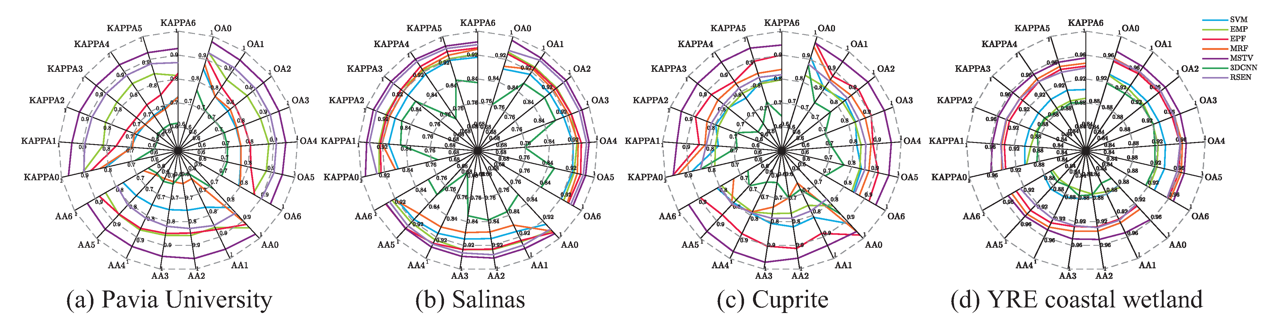
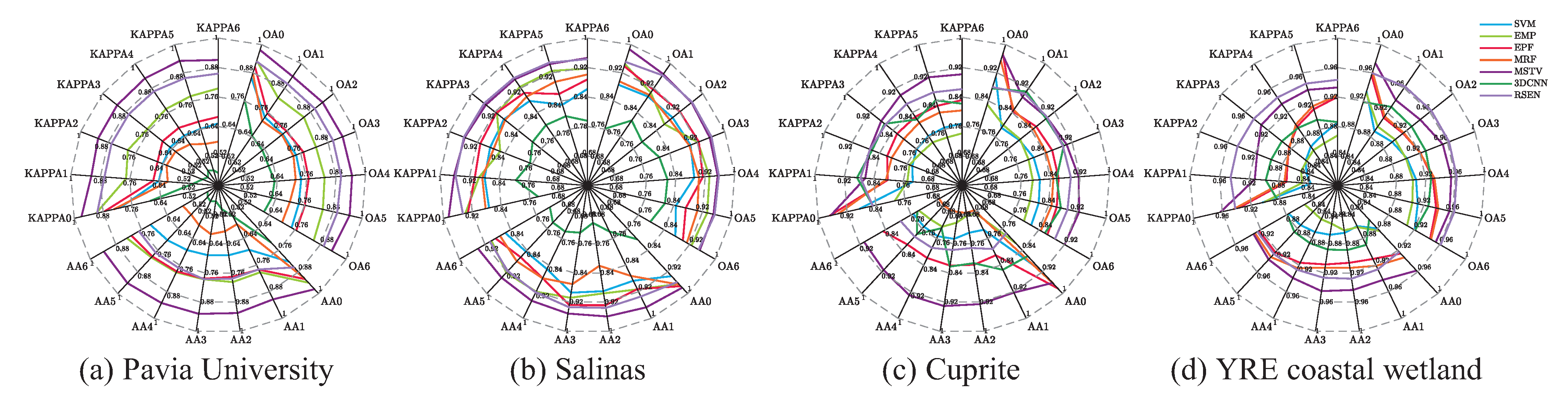
4.1. Effect Analysis of Single-Type Image Degradation

For the convenience of comparison and analysis, we graphically display the quantitative evaluation results of hyperspectral data with single-type degradation on a series of wind rose charts, where lines in different colors represent different classification methods. The three evaluation indices are rotated and arranged in a clockwise direction, and the end character 0–6 represents different degradation levels from low to high. In particular, level 0 reflects the classification performance of comparison methods on clean images. Since we are more concerned with the trend of the curves than with the specific values, the start and endpoints in each wind rose chart may vary slightly to maximize the curve trend.

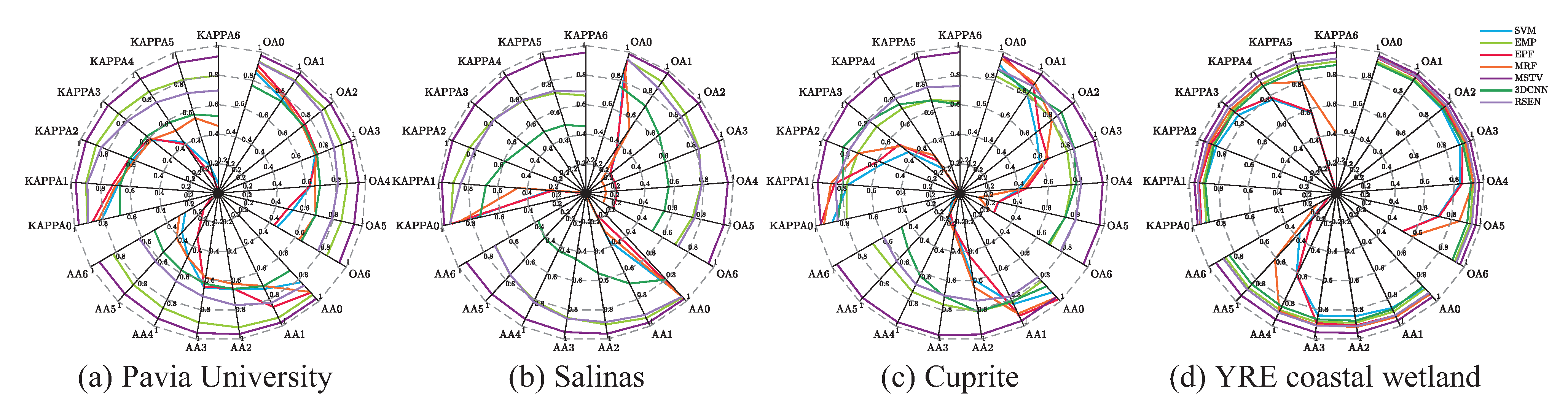
4.1.1. Effects of Low Spatial Resolution on Hyperspectral Image Classification

In order to study the effects of low spatial resolution on hyperspectral image classification, we displayed the results of four data in Figure 6. We can see that with the decrease in spatial resolution, the performance of different classification methods fluctuates in varying degrees on these four synthetic datasets. Among the seven methods, EPF, MRF, and MSTV perform more steadily than the rest of the methods. Due to the use of postprocessing steps, EPF and MRF can recover the problem of edge loss in the preliminary classification map, which makes the reduction of spatial resolution have little effect on EPF and MRF. MSTV considers multiscale features through upsampling and downsampling operations, so the results can also remain stable. It is interesting to note that the accuracy of the SVM method is improved when the spatial resolution is reduced because the intraclass differences of spectra can be reduced to a certain extent with the decrease of spatial resolution, which helps the SVM to better utilize the spectral information for classification. On the contrary, the accuracy of EMP is greatly affected by spatial resolution since the construction of morphological profiles heavily relies on the spatial information of the input image. A 3DCNN is a data-driven method that extracts features by multilayer convolution and pooling. Low spatial resolution affects the extraction of shallow features such as edge and texture, which in turn affects the classification accuracy. An RSEN extracts higher dimensional spatial features as the corresponding neighbor region of each original spectral vector and then trains them in both networks so that the results remain relatively robust to the reduction of spatial resolution.
From the four pictures in Figure 6, the accuracy of these less stable methods experiences the most obvious decline on Pavia University, because there exist many small and scattered objects with fine spatial features, which will have a great impact on their recognition once the spatial resolution is reduced. However, Salinas and YRE coastal wetland are composed of large-scale and regularly shaped land or water, so they do not rely on high spatial resolution to complete the classification task and the reduction of spatial resolution has less impact on their classification accuracy. Such comparison results reveal that low spatial resolution does not necessarily affect the performance of HSI classification, but it does when the spatial resolution is insufficient to match the feature scale.

4.1.2. Effects of Gaussian Noise on Hyperspectral Image Classification

The classification results of different methods under Gaussian noise degradation are displayed in Figure 7. It can be observed that, with the increase of the Gaussian noise level, the classification accuracy of all the methods decreases in different datasets, which reflects that Gaussian noise degradation has a universal adverse impact on hyperspectral classification. Among them, the methods with the most obvious decline in accuracy are the SVM, EPF, and MRF. Since the Gaussian noise disturbs the spectral characteristic, the spectral-based method SVM cannot perform well. As for the postprocessing-based methods EPF and MRF, their accuracy curves tend to decline as the SVM does, for the spectral-based methods’ first step is often to obtain the initial classification results. The accuracy of the EMP, 3DCNN, and RSEN also decreases, but it is not as obvious as the aforementioned three methods. This is because the feature calculation of the EMP is based on the most significant principal components of the hyperspectral data and the 3DCNN and RSEN employ the multiple-convolution technique, which can reduce the influence of Gaussian noise to a certain extent. In contrast, MSTV performs more robustly when different levels of Gaussian noise are added since the use of total variation can resist the effect of noise to the greatest extent.
When comparing the classification results on different data, Salinas stands out for its severest vulnerability to the synthetic Gaussian noise, as we can see the corresponding accuracy curves drop sharply in Figure 7b. Salinas represents data of farmland scenes with a variety of ground object types and minor interclass differences. Therefore, the classification accuracy on such data is often more sensitive to Gaussian noise.

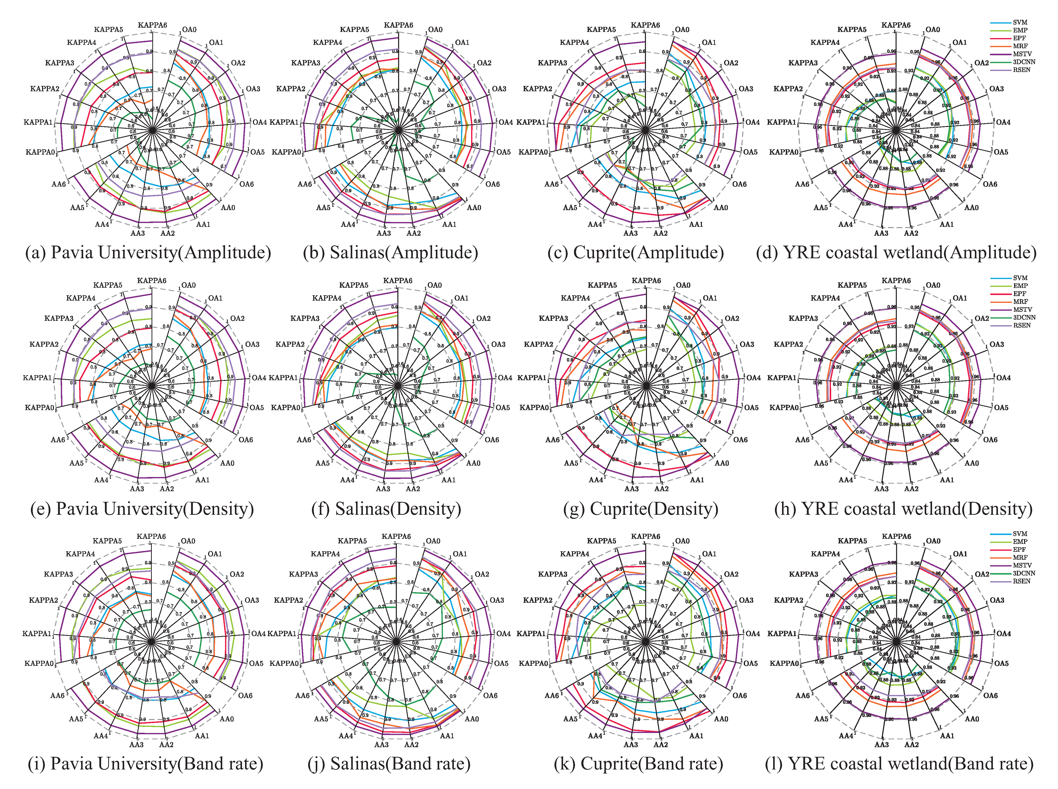
4.1.3. Effects of Stripe Noise on Hyperspectral Image Classification

The comparison of the classification accuracy of different methods on the synthetic stripe dataset is shown in Figure 8. Similar to Gaussian noise, stripe noise also has a general negative impact on the classification accuracy of hyperspectral images. Specifically, with the increase of stripe degradation level, including the amplitude, density, and the proportion of affected bands, the classification accuracy apparently decreases with more striped artifacts occurring in the classification results. Different from the random distribution of Gaussian noise, the distribution of stripe noise follows a certain law, which forms new spatial features in synthetic datasets. This makes EMP and the 3DCNN less robust to stripe noise than to Gaussian noise. For example, in EMP, the existence of stripe noise affects the construction of morphological profiles. Note that, among the three variables of stripe noise, the classification accuracy of the 3DCNN is more robust to the ratio of affected bands. This indicates that the architecture of 3D convolutions, which process spatial and spectral information simultaneously in deep learning methods, has a certain anti-interference capability to stripes occurring in part of the bands of hyperspectral data. MSTV still keeps stable performance for its multiscale and total variation strategy. The RSEN performs robustly here due to the cotraining of high-dimensional features from spectral and spatial domains in the base network and the ensemble network. Moreover, the filtering strategy on the corresponding probability vectors in the RSEN can also help resist noise to a certain extent.
From the perspective of comparing different datasets in Figure 8, we can find that the accuracy curves of Salinas and Cuprite drop significantly, which refers to a higher sensitivity to the stripe degradation, while the curves of YRE coastal wetland are more stable. On the one hand, there are small gaps between the features of different ground objects in Salinas and Cuprite. On the other hand, YRE coastal wetland has a higher proportion of labeled ground truth, which makes its training process more comprehensive and accurate. Undoubtedly, getting more accurate ground truth labels is also a way to resist noise interference.

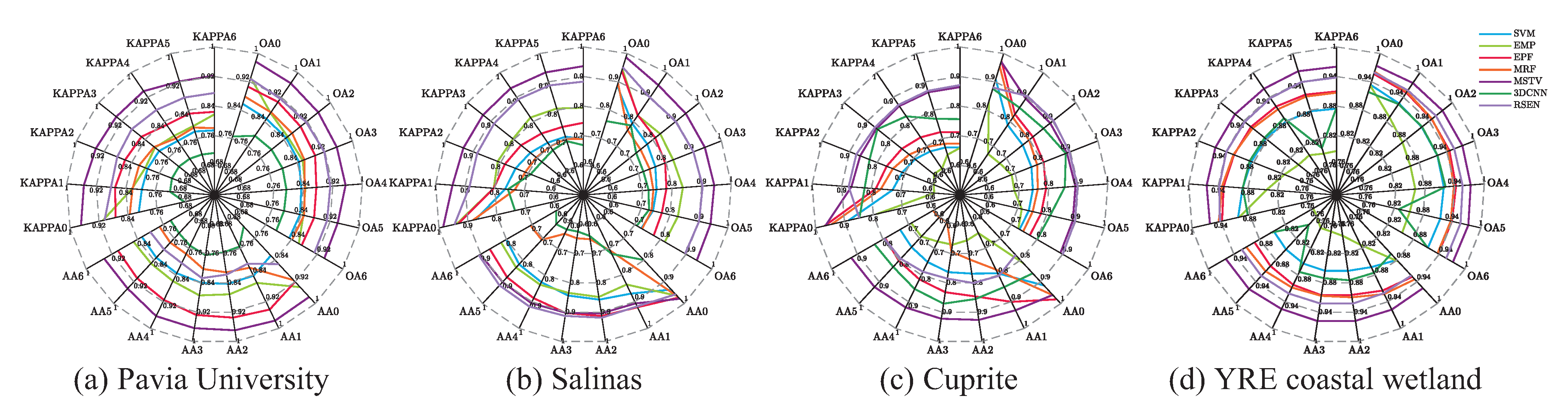
4.1.4. Effects of Fog on Hyperspectral Image Classification

Comparative experiments of seven methods were conducted on the synthetic datasets of fog, and the results are shown in Figure 9. It can be seen that adding fog to the image according to the physical model slightly reduced the accuracy of the seven HSI classification methods. When we simulated the fog datasets following [4], we used the fixed fog spectrum curve. Therefore, the spectrum of a degraded foggy pixel was a linear combination of the ground object spectrum and the fixed fog spectrum, which may only have a limited impact on the classification method based on spectral information. As the ground truth was still accurate, the classifier that adopted spectral information could still learn the characteristics of different ground feature categories for classification, with a small proportion of error.
Considering that in a real scene, the fog can sometimes be too thick to distinguish the accurate ground truth of objects, we conducted another set of experiments to verify the results in line with actual situations. Different from the assumption that the correct labels of the ground surface could always be obtained, we masked the ground truth where the fog intensity F was too high (see Figure 10). By adopting the original ground truth as the reference, the corresponding experimental results are shown in Figure 11. We can find that the classification accuracy of most methods is significantly reduced. This is because the seriously degraded areas lack ground truth values, which makes the classifier unable to fully learn the real features of various ground objects, and fog complicates the features of various categories. Moreover, the accuracy curve decreases rapidly from no degradation to degradation with fog, but the change is relatively stable under different degrees of fog. This shows that fog degradation has a negative impact on the classification accuracy of hyperspectral images, while under the same ground truth acquisition condition, the density of fog has less impact on the classification accuracy.

4.1.5. Effects of Shadow on Hyperspectral Image Classification

Based on the fog degradation experiments, we carried out two groups of shadow degradation experiments on HSIs in the same way. Figure 12 shows the results by using the original ground truth, while Figure 13 shows the results by using the ground truth which discards those areas with serious shadow degradation. The masked ground truth is shown in Figure 14. From Figure 12 and Figure 13, we can see that the classification accuracy is reduced after the image is affected by shadow. Compared with the situation when the ground truth under severe shadow still exists, the accuracy decreases more dramatically when part of the ground truth is lost. Due to a more labeled proportion of ground truth, the hyperspectral classification accuracy of Salinas and YRE coastal wetland is relatively stable in the shadow experiment series. Combined with the fog experiment series, these results show that when the clean image is affected by atmospheric interference, such as cloud, fog, shadow, and smoke, the most important factor affecting the classification accuracy is the visibility of the ground truth. If a high proportion of ground truth can still be obtained, the impact of atmospheric interference on classification accuracy is limited.

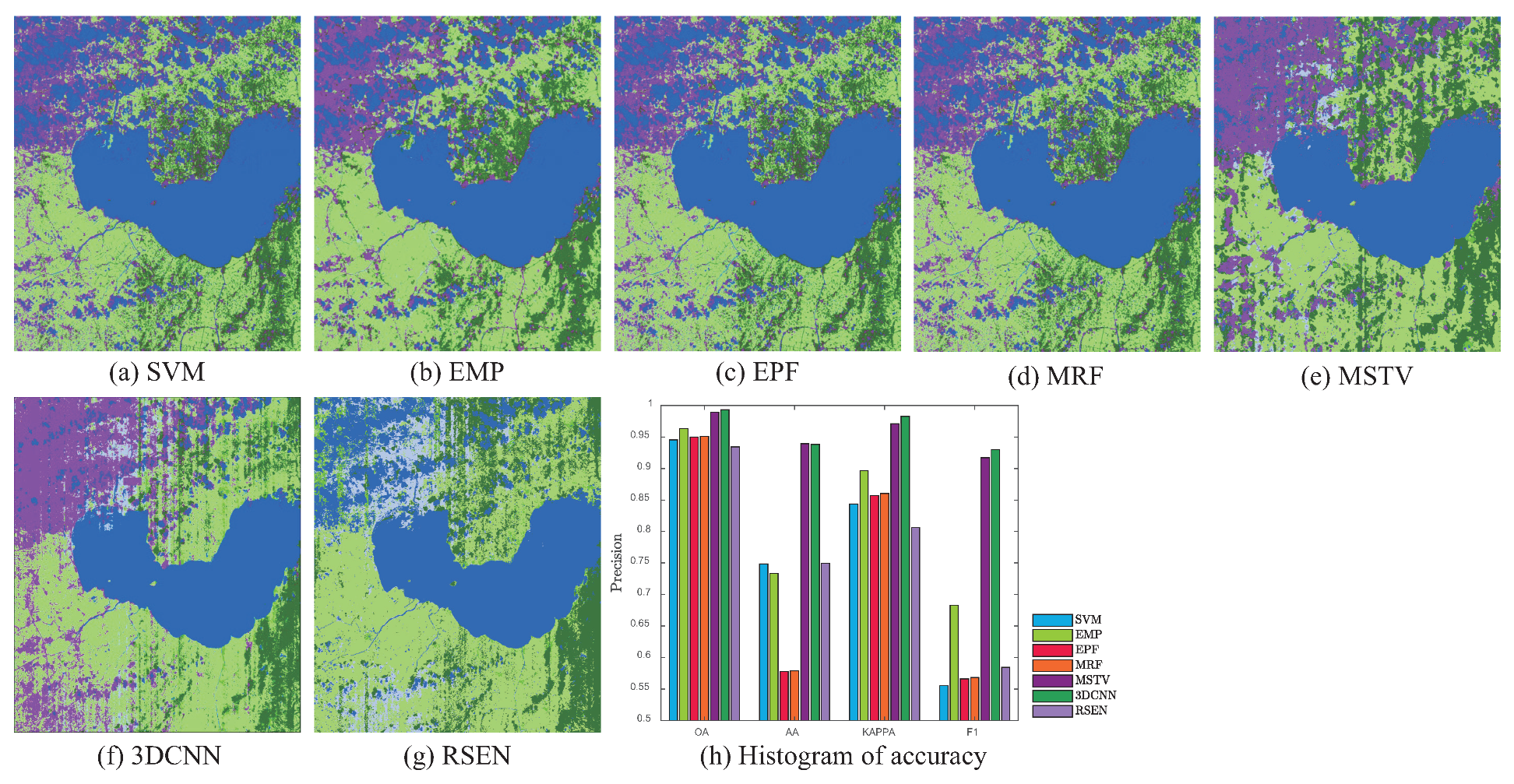
4.2. Effect Analysis of Mixed-Type Image Degradation

Classification results of seven comparative methods are shown in Figure 15. From the visual performance in Figure 15a–g, the water and cropland in the middle are well recognized by all the methods, but the impervious surface regions have worse classification results and unclear boundaries. This indicates that the 10 m spatial resolution of the Chaohu data is suitable for classifying large-scale water and cropland but is insufficient to depict the scattered impervious surface. As for the effects of Gaussian and stripe noise, it can be found that the overall negative impact on classification performance is consistent with the simulation experiment since noise artifacts are more or less distributed in the classification results of the sevenmethods. When comparing different categories in the same map, the lake region most affected by stripe noise has the best visual classification result. It is understandable as the category “Water” possesses a much higher proportion of labeled ground truth, which helps to resist noise interference. However, for the category with a low labeled proportion such as cropland, the spatial–spectral based hybrid method is more susceptible to the interference of stripe noise. This is because random stripes in HSIs interfere with spatial information more than spectral information, and the spatial–spectral hybrid methods lack the step of classification using spectral information alone. Additionally, the Chaohu data cover a large area of thick clouds and shadows. These two types of image degradation (associated with atmospheric interference) affect the performance of all the methods to varying degrees by misclassifying clouds and shadows as water. Among them, the hybrid methods including MSTV and the 3DCNN are relatively less affected. However, the RSEN completely misclassifies the category “Impervious Surface” in Figure 15g. This is because the RSEN refers to the balanced ground truth labels during training to realize reliable self-ensembling learning, while the real data may not meet this condition.
The corresponding quantitative assessment is shown in Figure 15h Limited by unbalanced labels, the RSEN fails to give full play to its advantages in real-data experiments. Althoughthe 3DCNN possesses lower accuracy curves than other methods in the simulation experiments, its classification accuracy is significantly improved due to the increase of training samples in the real-data experiment. In line with the simulation experiments where hybrid methods were more robust in most degradation cases, the 3DCNN and MSTV show a good stability to real mixed degraded data and obtain the top two classification performance values. According to the above experiments, we can see that the effects of image degradation on classification generally show good consistency between real-data and simulated experiments. Therefore, the effects of mixed degradation on classification can be regarded as the comprehensive effects of various image degradation problems.

5. Discussion

In this section, combing the results above, we provide suggestions on method selection and data preparation to handle degraded HSIs in classification tasks.

5.1. Method Selection to Handle Degraded HSIs in Classification

In terms of dealing with different HSI degradation, spectral-based methods, represented by SVMs, were more unstable. The addition of noise, fog, and shadow made the classification result of SVMs much worse because these degradations, without exception, interfered with the spectral information. Low spatial resolution, however, did not necessarily lead to the decline in classification accuracy of SVMs, and could even improve the classification due to the reduction of the intraclass spectral variability with the decrease of spatial resolution.
As for the spectral–spatial methods, the preprocessing-based method EMP was more sensitive to the degradations which were more relevant to spatial information, such as low spatial resolution, stripe noise with a special spatial distribution, and fog and shadow with irregular shapes. The reason was that the changes in spatial information caused by degradations adversely affected the construction of extended morphological profiles. EPF and MRF could maintain relatively stable performance when the spatial resolution of the input image decreased since they had the ability to deal with spatial edges and holes through the postprocessing step. However, when noise, fog, and shadow were added, the accuracy curves of the postprocessing-based methods fell along with that of the SVM method, as the SVM often acted as their first step. The hybrid methods MSTV, 3DCNN, and RSEN, were most robust in most degradation cases, for the total variation, multilayer 3D convolution strategies, and cotraining strategies with higher dimensional spatial and spectral features are designed to better characterize the image features and resist the influences from degradation factors. Unfortunately, there are exceptions. For example, when the label proportion for one category is very low, the hybrid methods may also perform poorly, such as regarding the relevant stripe degradation as meaningful edges and generating stripe artifacts in classification maps or even missing this category. In addition, the 3DCNN is a typical data-driven method that needs a certain number of training samples to obtain a satisfying classification result. Faced with the problem of HSI degradation, the model-based hybrid methods are suggested when training samples are limited, whereas the data-driven hybrid methods can be more suitable when the number of training samples is sufficient.

5.2. Data Preparation to Handle Degraded HSI in Classification

Comparing the four hyperspectral data in different scenes with their characteristics in experiments of HSIs with single-type degradation, the classification accuracy of Salinas and YRE coastal wetland was less sensitive to the reduction of the spatial resolution, while for Cuprite, it was the opposite. This is because the distribution of minerals in Cuprite is irregular and discontinuous, but the farmland and wetland scenes in Salinas and YRE coastal wetland have a continuous and large-scale distribution which does not rely much on the high spatial resolution for classification. This implies that it is necessary to select an image with the proper spatial resolution that matches the content of the scene to classify, namely, a scene with finer objects needs an image with a higher spatial resolution. When encountering Gaussian and stripe noise, the classification accuracy of all four datasets was reduced more or less, and noise artifacts appeared in the classification maps from real-data experiments. If possible, it is suggested to perform image denoising before classification for noisy inputs. When input images are degraded by fog or shadow, the degree of impact on the classification accuracy depends on whether the ground truth of the occluded area can be obtained. Therefore, it is not recommended to use images as classification input if the intensity of the fog or shadow is too strong to obtain a valid ground truth in the occluded area. Conversely, if the ground truth under fog or shadow can still be obtained, some classification methods may still get acceptable results after reasonable and effective training. Furthermore, among the four HSI data, we could find that the classification accuracy of all the compared methods fluctuated little for most types of degradation in YRE coastal wetland, because its proportion of labeled ground truth was much higher. This indicated that increasing the proportion of known accurate ground truth was also an effective way to improve the performance of the classifier. When degraded hyperspectral images are inevitably used for classification in practical applications, all the issues might exist simultaneously, which means the degradation of real images is more complicated. As for dealing with the mixed degradation problem in real classification tasks, there are two recommended ways. One is to restore the mixed degraded hyperspectral image before classification and the other is to use an anti-interference classification method. The former restores the mixed degraded hyperspectral images by sequentially using targeted image processing methods, such as super-resolution, denoising, de-striping, cloud removal, and shadow removal methods, or by directly using a well-trained end-to-end hybrid image restoration network. The latter reduces the influence of image degradation by combining the fusion technique with the aid of auxiliary data. End users are suggested to make corresponding choices according to the specific technologies they have mastered.

6. Conclusions

In this paper, we conducted comprehensive experiments to explore the influence of degraded hyperspectral data on the performance of existing hyperspectral image classification methods. We made a quantitative evaluation on a large number of classification results on hyperspectral data with single-type and mixed-type degradation. We synthesized a large number of degraded images with single-type degradation based on four scenes of clean hyperspectral datasets for training and testing, including images with low spatial resolution, images with Gaussian noise, images with stripe noise, images with fog, and images with shadow. Each degradation type had six degradation levels. To verify consistency, real-data experiments with mixed-type degradation were also conducted. We found that when hyperspectral images were degraded in most cases, the image classification performance declined to varying degrees. Specifically, low spatial resolution had an impact on hyperspectral classification, but the specific impact varied with the feature scale in the classification tasks. Comparative methods that mainly relied on spatial information could be affected more significantly. The existence of Gaussian noise generally reduced the classification performance of hyperspectral images, but strategies such as total variance and multilayer convolutions could effectively resist interference from it. Similar to Gaussian noise, stripe noise also had an overall negative impact on the performance of hyperspectral classification, of which three important factors all deserved attention. The effect of occlusion during imaging, such as fog and shadow, on the classification performance of hyperspectral images mainly depended on whether the ground truth of the surface in the degraded area could be obtained accurately. The ground truth of the degraded area enabled the classifier to get more comprehensive features and be trained more reliably, so as to obtain better classification results. Due to their outperforming effectiveness and stability, hybrid classification methods are recommended for dealing with HSI degradation. In addition, the same level of degradation had different effects on the classification performance of different hyperspectral classification tasks, which was related to the characteristics of the data, such as the size of ground features in the image, the proportion of labeled ground truth, the classification hierarchy, and so on. These findings provide a reference for researchers to select and develop more targeted methods in practical application scenarios. Developing and improving hyperspectral image classification methods to accommodate complex degradation interference in real applications will become a research hotspot in the future.

Author Contributions

Conceptualization, C.L., Z.L., and X.L.; methodology, C.L., Z.L., and X.L.; software, C.L. and X.L.; validation, C.L. and X.L.; formal analysis, C.L. and X.L.; data curation, C.L. and X.L.; writing—original draft preparation, C.L. and X.L.; writing—review and editing, C.L. and X.L.; visualization, C.L. and X.L.; supervision, X.L. and S.L.; project administration, X.L. and S.L. All authors have read and agreed to the published version of the manuscript.

Funding

This research was funded by the National Natural Science Foundation of China under Grants 61901166, 62221002, 61890962, and 41901280 and the Natural Science Foundation of Hunan Province of China under Grants 2022JJ40054 and 2020GK2038.

Data Availability Statement

The data presented in this study are openly available at https://github.com/hnulcy/datasets-for-comparative-study (accessed on 1 September 2022).

Conflicts of Interest

The authors declare no conflict of interest.

References

  1. Bioucas-Dias, J.M.; Plaza, A.; Camps-Valls, G.; Scheunders, P.; Nasrabadi, N.; Chanussot, J. Hyperspectral Remote Sensing Data Analysis and Future Challenges. IEEE Geosci. Remote Sens. Mag. 2013, 1, 6–36. [Google Scholar] [CrossRef] [Green Version]
  2. Shaw, G.; Manolakis, D. Signal processing for hyperspectral image exploitation. IEEE Signal Process. Mag. 2002, 19, 12–16. [Google Scholar] [CrossRef]
  3. Zare, A.; Ho, K. Endmember Variability in Hyperspectral Analysis: Addressing Spectral Variability During Spectral Unmixing. IEEE Signal Process. Mag. 2014, 31, 95–104. [Google Scholar] [CrossRef]
  4. Kang, X.; Fei, Z.; Duan, P.; Li, S. Fog Model-Based Hyperspectral Image Defogging. IEEE Trans. Geosci. Remote Sens. 2021, 60, 5512512. [Google Scholar] [CrossRef]
  5. Ghamisi, P.; Yokoya, N.; Li, J.; Liao, W.; Liu, S.; Plaza, J.; Rasti, B.; Plaza, A. Advances in Hyperspectral Image and Signal Processing: A Comprehensive Overview of the State of the Art. IEEE Geosci. Remote Sens. Mag. 2017, 5, 37–78. [Google Scholar] [CrossRef] [Green Version]
  6. Li, C.; Liu, X.; Kang, X.; Li, S. A Comparative Study of Noise Sensitivity on Different Hyperspectral Classification Methods. In Proceedings of the 2021 IEEE International Geoscience and Remote Sensing Symposium IGARSS, Brussels, Belgium, 11–16 July 2021; pp. 3689–3692. [Google Scholar] [CrossRef]
  7. Melgani, F.; Bruzzone, L. Classification of hyperspectral remote sensing images with support vector machines. IEEE Trans. Geosci. Remote Sens. 2004, 42, 1778–1790. [Google Scholar] [CrossRef] [Green Version]
  8. Zhong, Y.; Zhang, L. An Adaptive Artificial Immune Network for Supervised Classification of Multi-/Hyperspectral Remote Sensing Imagery. IEEE Trans. Geosci. Remote Sens. 2012, 50, 894–909. [Google Scholar] [CrossRef]
  9. Ham, J.; Chen, Y.; Crawford, M.; Ghosh, J. Investigation of the random forest framework for classification of hyperspectral data. IEEE Trans. Geosci. Remote Sens. 2005, 43, 492–501. [Google Scholar] [CrossRef] [Green Version]
  10. Fisher, R.A. The Use of Multiple Measurements in Taxonomic Problems. Ann. Hum. Genet. 2012, 7, 179–188. [Google Scholar] [CrossRef]
  11. Bandos, T.V.; Bruzzone, L.; Camps-Valls, G. Classification of Hyperspectral Images with Regularized Linear Discriminant Analysis. IEEE Trans. Geosci. Remote Sens. 2009, 47, 862–873. [Google Scholar] [CrossRef]
  12. Khodadadzadeh, M.; Li, J.; Plaza, A.; Bioucas-Dias, J.M. A Subspace-Based Multinomial Logistic Regression for Hyperspectral Image Classification. IEEE Geosci. Remote Sens. Lett. 2014, 11, 2105–2109. [Google Scholar] [CrossRef]
  13. Liew, S.C.; Chang, C.W.; Lim, K.H. Hyperspectral land cover classification of EO-1 Hyperion data by principal component analysis and pixel unmixing. In Proceedings of the IEEE International Geoscience and Remote Sensing Symposium, Toronto, ON, Canada, 24–28 June 2002; Volume 6, pp. 3111–3113. [Google Scholar] [CrossRef]
  14. Villa, A.; Benediktsson, J.A.; Chanussot, J.; Jutten, C. Hyperspectral Image Classification With Independent Component Discriminant Analysis. IEEE Trans. Geosci. Remote Sens. 2011, 49, 4865–4876. [Google Scholar] [CrossRef] [Green Version]
  15. Hughes, G. On the mean accuracy of statistical pattern recognizers. IEEE Trans. Inf. Theory 1968, 14, 55–63. [Google Scholar] [CrossRef] [Green Version]
  16. He, L.; Li, J.; Liu, C.; Li, S. Recent Advances on Spectral–Spatial Hyperspectral Image Classification: An Overview and New Guidelines. IEEE Trans. Geosci. Remote Sens. 2018, 56, 1579–1597. [Google Scholar] [CrossRef]
  17. Jia, X.; Kuo, B.C.; Crawford, M.M. Feature Mining for Hyperspectral Image Classification. Proc. IEEE 2013, 101, 676–697. [Google Scholar] [CrossRef]
  18. Chen, Y.; Nasrabadi, N.M.; Tran, T.D. Hyperspectral Image Classification Using Dictionary-Based Sparse Representation. IEEE Trans. Geosci. Remote Sens. 2011, 49, 3973–3985. [Google Scholar] [CrossRef]
  19. Fang, L.; Li, S.; Kang, X.; Benediktsson, J.A. Spectral–Spatial Hyperspectral Image Classification via Multiscale Adaptive Sparse Representation. IEEE Trans. Geosci. Remote Sens. 2014, 52, 7738–7749. [Google Scholar] [CrossRef]
  20. Benediktsson, J.A.; Palmason, J.A.; Sveinsson, J.R. Classification of hyperspectral data from urban areas based on extended morphological profiles. IEEE Trans. Geosci. Remote Sens. 2005, 43, 480–491. [Google Scholar] [CrossRef]
  21. Marpu, P.R.; Pedergnana, M.; Dalla Mura, M.; Benediktsson, J.A.; Bruzzone, L. Automatic Generation of Standard Deviation Attribute Profiles for Spectral–Spatial Classification of Remote Sensing Data. IEEE Geosci. Remote Sens. Lett. 2013, 10, 293–297. [Google Scholar] [CrossRef]
  22. Camps-Valls, G.; Gomez-Chova, L.; Munoz-Mari, J.; Vila-Frances, J.; Calpe-Maravilla, J. Composite kernels for hyperspectral image classification. IEEE Geosci. Remote Sens. Lett. 2006, 3, 93–97. [Google Scholar] [CrossRef]
  23. Li, J.; Marpu, P.R.; Plaza, A.; Bioucas-Dias, J.M.; Benediktsson, J.A. Generalized Composite Kernel Framework for Hyperspectral Image Classification. IEEE Trans. Geosci. Remote Sens. 2013, 51, 4816–4829. [Google Scholar] [CrossRef]
  24. Lu, T.; Li, S.; Fang, L.; Jia, X.; Benediktsson, J.A. From Subpixel to Superpixel: A Novel Fusion Framework for Hyperspectral Image Classification. IEEE Trans. Geosci. Remote Sens. 2017, 55, 4398–4411. [Google Scholar] [CrossRef]
  25. Fang, L.; Li, S.; Duan, W.; Ren, J.; Benediktsson, J.A. Classification of Hyperspectral Images by Exploiting Spectral–Spatial Information of Superpixel via Multiple Kernels. IEEE Trans. Geosci. Remote Sens. 2015, 53, 6663–6674. [Google Scholar] [CrossRef] [Green Version]
  26. Ghamisi, P.; Maggiori, E.; Li, S.; Souza, R.; Tarablaka, Y.; Moser, G.; De Giorgi, A.; Fang, L.; Chen, Y.; Chi, M.; et al. New Frontiers in Spectral-Spatial Hyperspectral Image Classification: The Latest Advances Based on Mathematical Morphology, Markov Random Fields, Segmentation, Sparse Representation, and Deep Learning. IEEE Geosci. Remote Sens. Mag. 2018, 6, 10–43. [Google Scholar] [CrossRef]
  27. Li, J.; Bioucas-Dias, J.M.; Plaza, A. Spectral–Spatial Hyperspectral Image Segmentation Using Subspace Multinomial Logistic Regression and Markov Random Fields. IEEE Trans. Geosci. Remote Sens. 2012, 50, 809–823. [Google Scholar] [CrossRef]
  28. Khodadadzadeh, M.; Ghamisi, P.; Contreras, C.; Gloaguen, R. Subspace Multinomial Logistic Regression Ensemble for Classification of Hyperspectral Images. In Proceedings of the IGARSS 2018—2018 IEEE International Geoscience and Remote Sensing Symposium, Valencia, Spain, 22–27 July 2018; pp. 5740–5743. [Google Scholar] [CrossRef]
  29. Kang, X.; Li, S.; Benediktsson, J.A. Spectral–Spatial Hyperspectral Image Classification with Edge-Preserving Filtering. IEEE Trans. Geosci. Remote Sens. 2014, 52, 2666–2677. [Google Scholar] [CrossRef]
  30. Li, J.; Bioucas-Dias, J.M.; Plaza, A. Spectral–Spatial Classification of Hyperspectral Data Using Loopy Belief Propagation and Active Learning. IEEE Trans. Geosci. Remote Sens. 2013, 51, 844–856. [Google Scholar] [CrossRef]
  31. Ghamisi, P.; Plaza, J.; Chen, Y.; Li, J.; Plaza, A.J. Advanced Spectral Classifiers for Hyperspectral Images: A review. IEEE Geosci. Remote Sens. Mag. 2017, 5, 8–32. [Google Scholar] [CrossRef] [Green Version]
  32. Szegedy, C.; Liu, W.; Jia, Y.; Sermanet, P.; Reed, S.; Anguelov, D.; Erhan, D.; Vanhoucke, V.; Rabinovich, A. Going deeper with convolutions. In Proceedings of the 2015 IEEE Conference on Computer Vision and Pattern Recognition (CVPR), Boston, MA, USA, 7–12 June 2015; pp. 1–9. [Google Scholar] [CrossRef] [Green Version]
  33. Bordes, A.; Glorot, X.; Weston, J. Joint Learning of Words and Meaning Representations for Open-Text Semantic Parsing. In Proceedings of the Artificial intelligence and statistics, La Palma, Spain, 21–23 April 2012. [Google Scholar]
  34. Chen, Y.; Lin, Z.; Zhao, X.; Wang, G.; Gu, Y. Deep Learning-Based Classification of Hyperspectral Data. IEEE J. Sel. Top. Appl. Earth Obs. Remote Sens. 2014, 7, 2094–2107. [Google Scholar] [CrossRef]
  35. Chen, Y.; Zhao, X.; Jia, X. Spectral–Spatial Classification of Hyperspectral Data Based on Deep Belief Network. IEEE J. Sel. Top. Appl. Earth Obs. Remote Sens. 2015, 8, 2381–2392. [Google Scholar] [CrossRef]
  36. Krizhevsky, A.; Sutskever, I.; Hinton, G.E. ImageNet Classification with Deep Convolutional Neural Networks. Commun. ACM 2017, 60, 84–90. [Google Scholar] [CrossRef] [Green Version]
  37. Wei, H.; Yangyu, H.; Li, W.; Fan, Z.; Li, H. Deep Convolutional Neural Networks for Hyperspectral Image Classification. J. Sens. 2015, 2015, 258619. [Google Scholar]
  38. Makantasis, K.; Karantzalos, K.; Doulamis, A.; Doulamis, N. Deep supervised learning for hyperspectral data classification through convolutional neural networks. In Proceedings of the 2015 IEEE International Geoscience and Remote Sensing Symposium (IGARSS), Milan, Italy, 26–31 July 2015; pp. 4959–4962. [Google Scholar] [CrossRef]
  39. Romero, A.; Gatta, C.; Camps-Valls, G. Unsupervised Deep Feature Extraction for Remote Sensing Image Classification. IEEE Trans. Geosci. Remote Sens. 2016, 54, 1349–1362. [Google Scholar] [CrossRef] [Green Version]
  40. Zhao, W.; Du, S. Spectral–Spatial Feature Extraction for Hyperspectral Image Classification: A Dimension Reduction and Deep Learning Approach. IEEE Trans. Geosci. Remote Sens. 2016, 54, 4544–4554. [Google Scholar] [CrossRef]
  41. Ben Hamida, A.; Benoit, A.; Lambert, P.; Ben Amar, C. 3-D Deep Learning Approach for Remote Sensing Image Classification. IEEE Trans. Geosci. Remote Sens. 2018, 56, 4420–4434. [Google Scholar] [CrossRef] [Green Version]
  42. Chen, Y.; Jiang, H.; Li, C.; Jia, X.; Ghamisi, P. Deep Feature Extraction and Classification of Hyperspectral Images Based on Convolutional Neural Networks. IEEE Trans. Geosci. Remote Sens. 2016, 54, 6232–6251. [Google Scholar] [CrossRef]
  43. Yokoya, N.; Yairi, T.; Iwasaki, A. Coupled Nonnegative Matrix Factorization Unmixing for Hyperspectral and Multispectral Data Fusion. IEEE Trans. Geosci. Remote Sens. 2012, 50, 528–537. [Google Scholar] [CrossRef]
  44. Li, S.; Dian, R.; Fang, L.; Bioucas-Dias, J.M. Fusing Hyperspectral and Multispectral Images via Coupled Sparse Tensor Factorization. IEEE Trans. Image Process. 2018, 27, 4118–4130. [Google Scholar] [CrossRef]
  45. Dian, R.; Li, S. Hyperspectral Image Super-Resolution via Subspace-Based Low Tensor Multi-Rank Regularization. IEEE Trans. Image Process. 2019, 28, 5135–5146. [Google Scholar] [CrossRef]
  46. Lin, C.H.; Ma, F.; Chi, C.Y.; Hsieh, C.H. A Convex Optimization-Based Coupled Nonnegative Matrix Factorization Algorithm for Hyperspectral and Multispectral Data Fusion. IEEE Trans. Geosci. Remote Sens. 2018, 56, 1652–1667. [Google Scholar] [CrossRef]
  47. Dong, C.; Loy, C.C.; He, K.; Tang, X. Image Super-Resolution Using Deep Convolutional Networks. IEEE Trans. Pattern Anal. Mach. Intell. 2016, 38, 295–307. [Google Scholar] [CrossRef] [PubMed] [Green Version]
  48. Yang, J.; Wright, J.; Huang, T.S.; Ma, Y. Image Super-Resolution Via Sparse Representation. IEEE Trans. Image Process. 2010, 19, 2861–2873. [Google Scholar] [CrossRef] [PubMed]
  49. Tong, T.; Li, G.; Liu, X.; Gao, Q. Image Super-Resolution Using Dense Skip Connections. In Proceedings of the 2017 IEEE International Conference on Computer Vision (ICCV), Venice, Italy, 22–29 October 2017; pp. 4809–4817. [Google Scholar] [CrossRef]
  50. Mei, S.; Jiang, R.; Li, X.; Du, Q. Spatial and Spectral Joint Super-Resolution Using Convolutional Neural Network. IEEE Trans. Geosci. Remote Sens. 2020, 58, 4590–4603. [Google Scholar] [CrossRef]
  51. Liu, D.; Wang, Z.; Wen, B.; Yang, J.; Han, W.; Huang, T.S. Robust Single Image Super-Resolution via Deep Networks With Sparse Prior. IEEE Trans. Image Process. 2016, 25, 3194–3207. [Google Scholar] [CrossRef]
  52. Liu, X.; Shen, H.; Yuan, Q.; Lu, X.; Zhou, C. A Universal Destriping Framework Combining 1-D and 2-D Variational Optimization Methods. IEEE Trans. Geosci. Remote Sens. 2018, 56, 808–822. [Google Scholar] [CrossRef]
  53. Fischer, A.D.; Thomas, T.J.; Leathers, R.A.; Downes, T.V. Stable Scene-based Non-uniformity Correction Coefficients for Hyperspectral SWIR Sensors. In Proceedings of the 2007 IEEE Aerospace Conference, Big Sky, MT, USA, 3–10 March 2007; pp. 1–14. [Google Scholar] [CrossRef]
  54. Corsini, G.; Diani, M.; Walzel, T. Striping removal in MOS-B data. IEEE Trans. Geosci. Remote Sens. 2000, 38, 1439–1446. [Google Scholar] [CrossRef]
  55. Chen, J.; Shao, Y.; Guo, H.; Wang, W.; Zhu, B. Destriping CMODIS data by power filtering. IEEE Trans. Geosci. Remote Sens. 2003, 41, 2119–2124. [Google Scholar] [CrossRef]
  56. Tsai, F.; Chen, W.W. Striping Noise Detection and Correction of Remote Sensing Images. IEEE Trans. Geosci. Remote Sens. 2008, 46, 4122–4131. [Google Scholar] [CrossRef]
  57. Asner, G.; Heidebrecht, K. Imaging spectroscopy for desertification studies: Comparing AVIRIS and EO-1 Hyperion in Argentina drylands. IEEE Trans. Geosci. Remote Sens. 2003, 41, 1283–1296. [Google Scholar] [CrossRef]
  58. Rakwatin, P.; Takeuchi, W.; Yasuoka, Y. Stripe Noise Reduction in MODIS Data by Combining Histogram Matching with Facet Filter. IEEE Trans. Geosci. Remote Sens. 2007, 45, 1844–1856. [Google Scholar] [CrossRef]
  59. Shen, H.; Zhang, L. A MAP-Based Algorithm for Destriping and Inpainting of Remotely Sensed Images. IEEE Trans. Geosci. Remote Sens. 2009, 47, 1492–1502. [Google Scholar] [CrossRef]
  60. Bouali, M.; Ladjal, S. Toward Optimal Destriping of MODIS Data Using a Unidirectional Variational Model. IEEE Trans. Geosci. Remote Sens. 2011, 49, 2924–2935. [Google Scholar] [CrossRef]
  61. Liu, X.; Lu, X.; Shen, H.; Yuan, Q.; Jiao, Y.; Zhang, L. Stripe Noise Separation and Removal in Remote Sensing Images by Consideration of the Global Sparsity and Local Variational Properties. IEEE Trans. Geosci. Remote Sens. 2016, 54, 3049–3060. [Google Scholar] [CrossRef]
  62. Jia, J.; Zheng, X.; Guo, S.; Wang, Y.; Chen, J. Removing Stripe Noise Based on Improved Statistics for Hyperspectral Images. IEEE Geosci. Remote Sens. Lett. 2020, 19, 5501405. [Google Scholar] [CrossRef]
  63. Yang, D.; Yang, L.; Zhou, D. Stripe removal method for remote sensing images based on multi-scale variation model. In Proceedings of the 2019 IEEE International Conference on Signal Processing, Communications and Computing (ICSPCC), Dalian, China, 20–23 September 2019; pp. 1–5. [Google Scholar] [CrossRef]
  64. Behnood, R.; Paul, S.; Pedram, G.; Giorgio, L.; Jocelyn, C. Noise Reduction in Hyperspectral Imagery: Overview and Application. Remote Sens. 2018, 10, 482. [Google Scholar]
  65. Rasti, B.; Ulfarsson, M.O.; Ghamisi, P. Automatic Hyperspectral Image Restoration Using Sparse and Low-Rank Modeling. IEEE Geosci. Remote Sens. Lett. 2017, 14, 2335–2339. [Google Scholar] [CrossRef]
  66. Jiang, T.X.; Zhuang, L.; Huang, T.Z.; Bioucas-Dias, J.M. Adaptive Hyperspectral Mixed Noise Removal. In Proceedings of the IGARSS 2018—2018 IEEE International Geoscience and Remote Sensing Symposium, Valencia, Spain, 22–27 July 2018; pp. 4035–4038. [Google Scholar] [CrossRef]
  67. He, K.; Sun, J.; Tang, X. Single Image Haze Removal Using Dark Channel Prior. IEEE Trans. Pattern Anal. Mach. Intell. 2011, 33, 2341–2353. [Google Scholar] [CrossRef] [PubMed]
  68. Cai, B.; Xu, X.; Jia, K.; Qing, C.; Tao, D. DehazeNet: An End-to-End System for Single Image Haze Removal. IEEE Trans. Image Process. 2016, 25, 5187–5198. [Google Scholar] [CrossRef] [PubMed] [Green Version]
  69. Gao, Y.; Su, Y.; Li, Q.; Li, J. Single fog image restoration via multi-scale image fusion. In Proceedings of the 2017 3rd IEEE International Conference on Computer and Communications (ICCC), Chengdu, China, 13–16 December 2017; pp. 1873–1878. [Google Scholar] [CrossRef]
  70. Makarau, A.; Richter, R.; Müller, R.; Reinartz, P. Haze Detection and Removal in Remotely Sensed Multispectral Imagery. IEEE Trans. Geosci. Remote Sens. 2014, 52, 5895–5905. [Google Scholar] [CrossRef] [Green Version]
  71. Guo, Q.; Hu, H.M.; Li, B. Haze and Thin Cloud Removal Using Elliptical Boundary Prior for Remote Sensing Image. IEEE Trans. Geosci. Remote Sens. 2019, 57, 9124–9137. [Google Scholar] [CrossRef]
  72. Zhang, L.; Zhang, Q.; Xiao, C. Shadow Remover: Image Shadow Removal Based on Illumination Recovering Optimization. IEEE Trans. Image Process. 2015, 24, 4623–4636. [Google Scholar] [CrossRef] [PubMed]
  73. Khan, S.H.; Bennamoun, M.; Sohel, F.; Togneri, R. Automatic Shadow Detection and Removal from a Single Image. IEEE Trans. Pattern Anal. Mach. Intell. 2016, 38, 431–446. [Google Scholar] [CrossRef]
  74. Liu, Y.; Bioucas-Dias, J.; Li, J.; Plaza, A. Hyperspectral cloud shadow removal based on linear unmixing. In Proceedings of the 2017 IEEE International Geoscience and Remote Sensing Symposium (IGARSS), Fort Worth, TX, USA, 23–28 July 2017; pp. 1000–1003. [Google Scholar] [CrossRef]
  75. Zhang, G.; Cerra, D.; Muller, R. Towards the Spectral Restoration of Shadowed Areas in Hyperspectral Images Based on Nonlinear Unmixing. In Proceedings of the 2019 10th Workshop on Hyperspectral Imaging and Signal Processing: Evolution in Remote Sensing (WHISPERS), Amsterdam, The Netherlands, 24–26 September 2019; pp. 1–5. [Google Scholar] [CrossRef]
  76. Windrim, L.; Ramakrishnan, R.; Melkumyan, A.; Murphy, R.J. A Physics-Based Deep Learning Approach to Shadow Invariant Representations of Hyperspectral Images. IEEE Trans. Image Process. 2018, 27, 665–677. [Google Scholar] [CrossRef]
  77. Liu, D.; Cheng, B.; Wang, Z.; Zhang, H.; Huang, T.S. Enhance Visual Recognition Under Adverse Conditions via Deep Networks. IEEE Trans. Image Process. 2019, 28, 4401–4412. [Google Scholar] [CrossRef] [PubMed] [Green Version]
  78. Liu, X.; Wang, H.; Meng, Y.; Fu, M. Classification of Hyperspectral Image by CNN Based on Shadow Area Enhancement Through Dynamic Stochastic Resonance. IEEE Access 2019, 7, 134862–134870. [Google Scholar] [CrossRef]
  79. Luo, R.; Liao, W.; Zhang, H.; Zhang, L.; Scheunders, P.; Pi, Y.; Philips, W. Fusion of Hyperspectral and LiDAR Data for Classification of Cloud-Shadow Mixed Remote Sensed Scene. IEEE J. Sel. Top. Appl. Earth Obs. Remote Sens. 2017, 10, 3768–3781. [Google Scholar] [CrossRef]
  80. Fu, P.; Sun, Q.; Ji, Z.; Geng, L. A Superpixel-Based Framework for Noisy Hyperspectral Image Classification. In Proceedings of the IGARSS 2020—2020 IEEE International Geoscience and Remote Sensing Symposium, Waikoloa, HI, USA, 26 September– 2 October 2020; pp. 834–837. [Google Scholar] [CrossRef]
  81. Duarte-Carvajalino, J.M.; Castillo, P.E.; Velez-Reyes, M. Comparative Study of Semi-Implicit Schemes for Nonlinear Diffusion in Hyperspectral Imagery. IEEE Trans. Image Process. 2007, 16, 1303–1314. [Google Scholar] [CrossRef] [PubMed]
  82. Hu, Y.; Zhang, J.; Ma, Y.; An, J.; Ren, G.; Li, X. Hyperspectral Coastal Wetland Classification Based on a Multiobject Convolutional Neural Network Model and Decision Fusion. IEEE Geosci. Remote. Sens. Lett. 2019, 16, 1110–1114. [Google Scholar] [CrossRef]
  83. Keys, R. Cubic convolution interpolation for digital image processing. IEEE Trans. Acoust. Speech Signal Process. 1981, 29, 1153–1160. [Google Scholar] [CrossRef]
  84. Barrow, H.; Tenenbaum, J. Recovering Intrinsic Scene Characteristics From Images. Comput. Vis. Syst. 1978, 2, 3–26. [Google Scholar]
  85. Levin, A.; Lischinski, D.; Weiss, Y. A Closed-Form Solution to Natural Image Matting. IEEE Trans. Pattern Anal. Mach. Intell. 2008, 30, 228–242. [Google Scholar] [CrossRef] [Green Version]
  86. Tarabalka, Y.; Fauvel, M.; Chanussot, J.; Benediktsson, J.A. SVM- and MRF-Based Method for Accurate Classification of Hyperspectral Images. IEEE Geosci. Remote Sens. Lett. 2010, 7, 736–740. [Google Scholar] [CrossRef] [Green Version]
  87. Duan, P.; Kang, X.; Li, S.; Ghamisi, P. Noise-Robust Hyperspectral Image Classification via Multi-Scale Total Variation. IEEE J. Sel. Top. Appl. Earth Obs. Remote Sens. 2019, 12, 1948–1962. [Google Scholar] [CrossRef]
  88. Audebert, N.; Le Saux, B.; Lefevre, S. Deep Learning for Classification of Hyperspectral Data: A Comparative Review. IEEE Geosci. Remote Sens. Mag. 2019, 7, 159–173. [Google Scholar] [CrossRef] [Green Version]
  89. Xu, Y.; Du, B.; Zhang, L. Robust Self-Ensembling Network for Hyperspectral Image Classification. IEEE Trans. Neural Netw. Learn. Syst. 2022, 1–14. [Google Scholar] [CrossRef] [PubMed]
Figure 1. Examples of real degraded hyperspectral images. (a) was captured by the Advanced Hyperspectral Imager (AHSI) on the GF-5 satellite over Juzizhou in Changsha, China. (b) was obtained by the airborne hyperspectral imager Nano-Hyperspec with 270 continuous spectral bands over Wangcheng District in Changsha, China. (c) was captured by the AVIRIS sensor with 224 bands and is available from the Hyperspectral Defogging dataset (HDD) [4]. (d) is a subregion of Houston2013 data with 144 bands.
Remotesensing 14 05199 g001
Figure 2. The proposed analysis framework.
Remotesensing 14 05199 g002
Figure 3. Original clean HSIs with their ground truths.
Remotesensing 14 05199 g003
Figure 4. Hyperspectral dataset with single-type degradation.
Remotesensing 14 05199 g004
Figure 5. Chaohu data with mixed-type degradation.
Remotesensing 14 05199 g005
Figure 6. Accuracy comparison of different classification methods on synthetic HSIs under low spatial resolution degradation.
Remotesensing 14 05199 g006
Figure 7. Accuracy comparison of different classification methods on synthetic HSIs under Gaussian noise degradation.
Remotesensing 14 05199 g007
Figure 8. Accuracy comparison of different classification methods on synthetic HSIs under stripe noise degradation.
Remotesensing 14 05199 g008
Figure 9. Accuracy comparison of different classification methods on synthetic HSIs under fog degradation.
Remotesensing 14 05199 g009
Figure 10. Ground truth that discards areas severely affected by fog.
Remotesensing 14 05199 g010
Figure 11. Accuracy comparison of different classification methods on synthetic HSIs under fog degradation (with affected ground truth).
Remotesensing 14 05199 g011
Figure 12. Accuracy comparison of different classification methods on synthetic HSIs under shadow degradation.
Remotesensing 14 05199 g012
Figure 13. Accuracy comparison of different classification methods on synthetic HSIs under shadow degradation (with affected ground truth).
Remotesensing 14 05199 g013
Figure 14. Ground truth that discards areas severely affected by shadow.
Remotesensing 14 05199 g014
Figure 15. Classification performance of the various methods for Chaohu data.
Remotesensing 14 05199 g015
Publisher’s Note: MDPI stays neutral with regard to jurisdictional claims in published maps and institutional affiliations.

