Article

Double Deep Q-Network for Hyperspectral Image Band Selection in Land Cover Classification Applications

1
College of Information, Shanghai Ocean University, 999 Hucheng Huanlu, Shanghai 201308, China
2
School of Computer Science and Technology, Donghua University, 2999 North Renmin Road, Shanghai 201620, China
*
Author to whom correspondence should be addressed.
Remote Sens. 2023, 15(3), 682; https://doi.org/10.3390/rs15030682
Submission received: 2 December 2022 / Revised: 17 January 2023 / Accepted: 19 January 2023 / Published: 23 January 2023
(This article belongs to the Special Issue Advances in Hyperspectral Remote Sensing Image Processing)

Abstract

:
Hyperspectral data usually consists of hundreds of narrow spectral bands and provides more detailed spectral characteristics compared to commonly used multispectral data in remote sensing applications. However, highly correlated spectral bands in hyperspectral data lead to computational complexity, which limits many applications or traditional methods when applied to hyperspectral data. The dimensionality reduction of hyperspectral data becomes one of the most important pre-processing steps in hyperspectral data analysis. Recently, deep reinforcement learning (DRL) has been introduced to hyperspectral data band selection (BS); however, the current DRL methods for hyperspectral data BS simply remove redundant bands, lack the significance analysis for the selected bands, and the reward mechanisms used in DRL only take basic forms in general. In this paper, a new reward mechanism strategy has been proposed, and Double Deep Q-Network (DDQN) is introduced during BS using DRL to improve the network stabilities and avoid local optimum. To verify the effect of the proposed BS method, land cover classification experiments were designed and carried out to analyze and compare the proposed method with other BS methods. In the land cover classification experiments, the overall accuracy (OA) of the proposed method can reach 98.37%, the average accuracy (AA) is 95.63%, the kappa coefficient (Kappa) is 97.87%. Overall, the proposed method is superior to other BS methods. Experiments have also shown that the proposed method works not only for airborne hyperspectral data (AVIRIS and HYDICE), but also for hyperspectral satellite data, such as PRISMA data. When hyperspectral data is applied to similar applications, the proposed BS method could be a candidate for the BS preprocessing options.

1. Introduction

With the advance of imaging technology and the increasing demand of hyperspectral data for many applications, more hyperspectral satellites/sensors are developed and launched, such as HJ-1A [1], Zhuhai-1 [2], GaoFen-5 [3], DESIS [4], PRISMA [5], and the recently launched EnMAP [6]. The huge volume of hyperspectral data significantly increases computational inefficiency and also causes storage stress. In addition, the high resolution of the spectrum data leads to high correlations between adjacent bands and certain data redundancy. Therefore, dimensionality reduction, as an important pre-processing step of hyperspectral analysis, is important and usually necessary to eliminate redundant bands and increase computational efficiency [7].
Dimensionality reduction methods for hyperspectral data can be categorized into feature extraction and band selection (hereinafter abbreviated as BS). Feature selection is to extract a set of new feature vectors from the all available feature vectors through function mapping [8,9]. Popular feature extraction methods are Projection Pursuit [10], Principal Component Analysis (PCA) [11], maximum-variance PCA (mvPCA) [12], Wavelet Transform [13], Independent Component Analysis (ICA) [14], the latest feature extraction method of deep learning [15], and so on. These projected features retain most of the expected information, but change the physical meaning of data, and the original and projected information may be distorted [8]. In contrast to feature extraction, BS chooses a representative subset of the original hyperspectral bands without losing physical significance [16,17]. BS has the advantage of retaining relevant original information in the data and the data structures as well; therefore, BS methods attract more attention in many hyperspectral applications.
Based on using labelled samples or not using labelled samples during BS, BS can be further divided into supervised BS [18,19,20,21], semi-supervised BS [22,23,24,25,26], and unsupervised BS [27,28]. Supervised and semi-supervised BS methods use labelled samples to guide the selection process. However, because the acquisition of labelled samples is a difficult and sometimes challenge task, in recent years, many unsupervised BS methods have been proposed. The ranking method and clustering method are two kinds of popular unsupervised BS methods.
The ranking method assigns a ranking value to each band and simply selects the bands from high values to low values. This method is stable and effective. It first quantifies the significance (ranking value) of each band according to certain criteria, then sorts the significance from high to low, sets the ranking value as its weight, and finally selects the bands with the higher weights as the chosen bands. Based on ranking criteria, there are rank-based methods using non-Gaussian [8,29], variance [12], and mutual information [30]. The key point in the ranking methods is to accurately describe the significance of spectral bands. However, the ranking method suffers a drawback that quite often the high-ranking bands could be adjacent bands, therefore resultant highly correlation among selected bands.
Clustering method firstly partitions all bands into certain clusters, and then selects the most representative bands from each cluster to form a subset of bands [31,32]. There are clustering methods using affinity propagation [33], exemplar component analysis [34], K-means-based BS methods [35], and the adaptive density method [36]. The clustering method considers the interaction between bands, but there are always two inherent shortcomings in the clustering process: the selected subset of bands may be unstable since the clustering-based methods are sensitive to randomly selected initial centroids; and most of these clustering methods only consider the correlation between bands, ignoring the information content of the selected subset of bands [37].
Deep learning methods based on deep neural networks have attracted much attention in the visual community due to their hierarchical expression and good generalization abilities, and have been successfully adopted in the field of hyperspectral data [38,39,40,41]. This has inspired the community to develop various attention mechanisms that can not only indicate where the focus is, but also improve the quality of feature representation [42,43]. The band or channel attention module (CAM) was originally introduced in the BS network (BSNet-Conv) [44] to select most significant spectral bands carrying useful information for classification. However, BSNet-Conv captures remote contextual information weakly in both spatial and spectral directions. In addition, the existing BS methods cannot simultaneously consider the global nonlinear interaction between spectral information and spatial information of different bands.
Deep reinforcement learning (DRL) has been proven to be an effective, general-purpose technique to develop reasonably good policies in sequential decision-making problems. There are two recently published BS methods based on DRL [26,45]. The main idea of using DRL for BS is to treat BS as a Markov Decision Process (MDP) and adjust BS effects by changing the reward mechanism. Feng et al. [26] built an evaluation network, used the network loss function as Asynchronous Advantage Actor-Critic (A3C) reward mechanism to select bands, and then used deep neural network for classification. It only emphasized the effect of deep neural network classification algorithms, did not describe the advantage of A3C for BS. A3C is suitable for both continuous and discrete action environments, but their experiments did not reflect this in the authors’ opinion. Mou et al. [45] used information entropy as Deep Q-Network (DQN) reward mechanism for BS. Their method is suitable for discrete action environment. However, their method has obvious multiple descent phenomena, which is unstable during BS and easily leads to local optimum.
In this paper, a partially supervised Double DQN (DDQN) BS method is proposed. In this proposed method, the BS process is formalized as an MDP. In an MDP, each state is a subset of possible bands, and each action is to determine which band to be selected or end the selection. When computing the reward, the labeled data is used to calculate the contribution of each band for the classification problem, and the contribution value is treated as the reward in DRL. Therefore, the proposed method is a partially supervised BS method. Considering that BS process is discrete, DDQN is therefore used for BS instead of DQN. The main contributions of this study are as follows: (1) a new DRL BS method which uses DDQN as the reward updating mechanism to avoid local optima was proposed; (2) three reinforcement reward functions were compared to find the most suitable one for the proposed method and; (3) the labeled land cover classification data was used for the reward function, which is tailored for remote sensing classification applications.
The rest of this paper is organized as follows: Section 2 describes the details of the proposed method. Section 3 describes the experimental datasets: from AVIRIS, HYDICE, PRISMA and Sentinel-2 Multispectral remote sensor (MRS). Section 4 describes the experimental design. Section 5 describes the experimental results: The results of reward functions and the results of different BS methods comparison., and the discussions are given in Section 6. Finally, Section 7 is the conclusion.

2. Methods

The common techniques of BS for hyperspectral data are discussed in the previous section and their technical details can be found in their relevant literatures [26,45]. In this section only some the key concepts of DRL, which are tailored to the proposed BS method are described, the readers may find the background information and general knowledge about DRL from relevant sources such as [46]. In DRL, MDP acts as the basic mathematical model. A broad range of applications including BS can be treated as a MDP, therefore there are possibilities to employ DRL as a tool to solve the BS problems. MDP involves action, status, status transition, reward and discount factors γ which reflects the value proportion of future rewards at the current moment [47].
Action: this represents a limited set of actions. The agent is to select a spectral band from the hyperspectral data at each time step, including the end action. The complete set of all actions A is exactly the same as the band set. The band set size is L, which is the number of bands. There is a A , where a t represents the action at time t .
Status: the historical actions is used as status. It is represented by L-dimensional vector, and the vector value is multi-hot encoding. For example, s i = 1 represents that the i t h band has been selected in the previous time step, and s i = 0 represents has not been selected. Taking the action history as the state means that the dependency between bands is considered, which helps to select the next band.
Transition: if any action is selected, the state will transition from one state to another. This process is described as a state transition function. Specifically, band b i is selected from the remaining bands which have not been selected yet, the status s t will transition to the status s i + 1 . In new state s i + 1 , the corresponding i t h value of status vector is set to 1. If the selected action is stop, the state will transition to the terminal state and the round of selection will end. The transfer function is as follows:
s i + 1   =   T e r m i n a l ,   i f   a t = s t o p               s t + b i ,   i f   a t = s e l e c t   a   n e w   b a n d   o f   b i
Reward: this represents the feedback on actions for the environment.

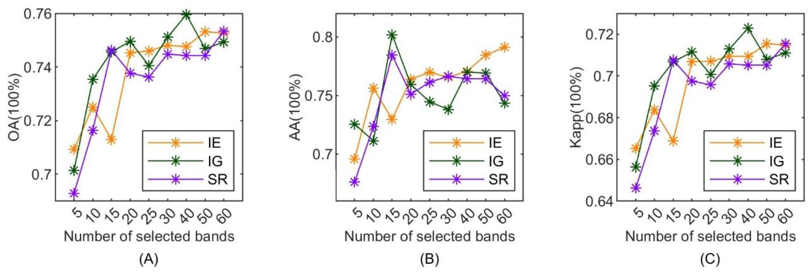
2.1. Reward Functions

Reward plays a vital role in DRL. It is common that using different reward functions will produce different results. Three reward functions were proposed for updating the reward scheme. The first reward function is information entropy (IE) [26]. IE can quantitatively measure the information of a random variable. In image processing, IE of an image can be defined according to the pixel value distribution of the image, which reflects the richness of image information. It is used to evaluate the abundance of spectral information. IE of each band is defined as the reward:
I E a = n = 1 N P x n log 2 P x n
where N represents the number of pixel values, x n represents the n t h pixel value. P is the proportion of the corresponding pixel value in the total number.
The second reward function is information gain (IG). Information gain is an important indicator of feature extraction. It is defined as how much information a feature can bring to the classification system [36]. The more information it brings, the more important the feature is, and therefore the greater the corresponding IE is. IG can be expressed by the form IE and conditional entropy. Conditional entropy represents the complexity of random variables under a certain condition. It is the probability of each classification under a certain band. IG of the corresponding band is given as follows:
I G C , B = H C H ( C | B )
H C = i = 1 N P x i log 2 P x i
H C | B = b B P b H ( C | B = b )
where I G C , B is the information gain of band feature B , it represents the reward value, C represents the category of labelled data, B represents the vector of the band. H C represents IE of the category, N represents the number of categories, and P represents the proportion of each category. H C | B is the conditional entropy, which represents the category entropy when the feature is B , P b is the overall proportion of each pixel value in feature B , and H ( C | B = b ) represents the information entropy of different categories when the pixel value is B . Because the labelled data was used for calculating IG, this reward is “supervised”.
The third reward function is termed as supervised reward (SR) by the authors, which is also “supervised” and uses random forest as the classifier. SR indirectly compute the reward scores using the classification accuracy derived from Random Forest (RF) classifier. During RF classification, only one band is eliminated each time, and L-1 bands are reserved (L represents the band number to be selected). The accuracy of RF is recorded as the weight of the band. The higher the accuracy, the less important the band is. The smaller the weight is, the more important the band is. The follow equation is used to compute the reward SR score:
S R = 1 A c c u r a c y
where S R is the reward score, A c c u r a c y is the classification accuracy derived from RF.
It can be seen from the reward mechanism, when the status transfers from s t to s t + 1 , if the band which has a great impact on classification is selected, this will give the enhancement of reward for this particular band, otherwise, the enhancement should be weakened. Driven by this reward scheme, the selected band has overall maximum value. The above three reward functions (IE, IG and SR) are compared at the beginning of the experiments to find which reward function works best for the proposed BS method.

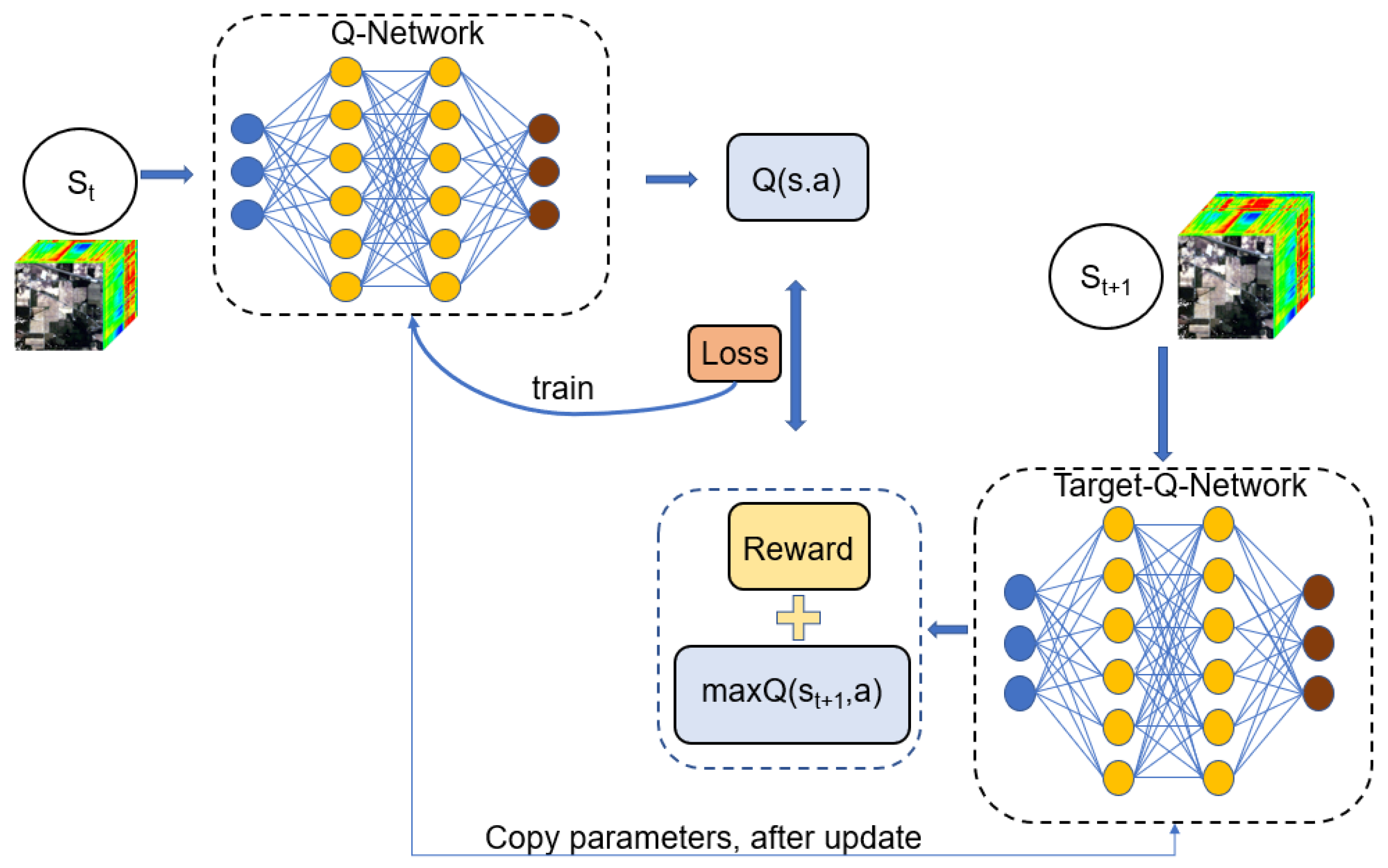
2.2. Double Deep Q Network (DDQN)

DRL uses Deep Q-Network (DQN) to represent the optimal action-value function as a neural network instead of using a Q-table. Its origin is back to 2015 DeepMind team leveraged the DQN that learned to play many Atari video games better than humans [48]. DQN approximates a state-value function in a Q-Learning framework. Taking the selected band history as the state, and DQN goes to the next status according to the state and the next action. Action selection adopts ε g r e e d y policy. In state S, the results of action a which is selected are determined by the maximum discount and reward, as shown in Equation (7):
Q s , a ; θ = E ( r t + γ r t + 1 + γ 2 r t + 2 + + | s t = s ,   a t = a )
where s is the current state, a is the action executed in the current state, θ is a network parameter, r t represents the reward when a is selected, γ is a discount factor. Select the action that maximizes Q .
Q s , a ; θ = max a   E ( r t + γ r t + 1 + γ 2 r t + 2 + + | s t = s ,   a t = a )
Suppose the state at time t + 1 is s t + 1 , then the DQN target value is:
y t   r t + γ max a   Q m s t + 1 ,   a t ; θ
The loss function of DQN is defined as:
L = E s , a , r , s ( y t Q m s , a ; θ ) 2
As many community shows that DQN suffers a major drawback from overestimation of Q-values in early stage while it’s still evolving [49,50]. In attempting to solve the local optimum problems caused by using DQN during select and evaluate actions, Double DQN (DDQN) is used instead to improve the probability of selecting optimal actions. There are two networks in DQN: evaluation network and target network. In DDQN, select actions are conducted through Q-network which is the evaluation network to determine the action, then evaluate actions are conducted through target Q-network, the rest of DDQN remains the same as DQN. DDQN only needs to use the evaluation network to determine the action and the target network to determine the action value. Therefore, it is only necessary to change the target value in DQN:
y t = r t + γ Q ( s t + 1 , a r g m a x a   Q ( s t + 1 ,   a t ; θ ) ; θ )
where y is the target value, γ is a discount factor, θ is the evaluation network parameter, θ is the target network parameter. DDQN replaces the above DQN loss function, fits Q value and train parameters.
The DDQN pseudo code is shown in Algorithm 1, the framework is shown in Figure 1. Since the core algorithm of DRL-Mou [45] is DQN and the proposed method uses DDQN, therefore the DQN and DDQN comparisons are made through DRL-Mou method and the proposed method. During training process and environment fitting, DDQN will learn a BS strategy and guide to select the bands. No matter in the training process or the testing process, the agent will not select the already selected bands. In the training phase, the initial state is empty. In the test phase, the initial state is randomly selected, any band could be in the initial state. It is hoped that an optimal subset of bands can be found from this mechanism.
Algorithm 1 Double DQN
1: Input: randomly initialize Q-network weights θ, copy θ to θ’; initialize replay memory M; initialize the complete set of all actions A; load reward table R;
2: for e = 0 ; e < E ;  do
3:        initialize state: s
4:        empty the set of chosen bands: B
5:         for   t = 0 ; t < K ;  do
6:                compute the actual set of actions, simulate one step with the ε-greedy policy;
7:                choose action a;
8:                             a ,   s t + 1 ,   r = S T E P T s , a ;
9:                               add   the   experience   ( s ,   a ,   r ,   s t + 1 ) into M;
10:                             s s t + 1 ;
11:        end for
12:        randomly sample a mini-batch Bc from M;
13:        for   ( s ,   a ,   r ,   s t + 1 ) ϵ B c  do
14:               calculate the learning target according to Equation (11)
15:               y t = r t + γ Q ( s t + 1 , a r g m a x a Q s t + 1 ,   a t ; θ ; θ )
16:        end for
17:        carry out a gradient descent step on L, according to Equation (10)
18:        L = E s , a , r , s ( y t Q m s , a ; θ ) 2
19:         update   Q - network   θ , θ  
20: end for

2.3. The Proposed DDQN Based BS Method

The proposed BS method uses DDQN as the backbone. It contains two networks: Q-network and target Q-network. Q-network is for training parameters, the construct of target Q-network is the same as Q-network. In Q-network, the input consists of a L-dimensional vector. The first fully connected layer has 2 L units, followed by rectifier linear units, the function is ReLUs. In the last layer, a linear fully connected layer with L units. In the practical experiments, the size of the playback memory is set to 10,000 and used 100 as the batch size. ε g r e e d y starts from 0.9 and gradually drops to 0.01 during iterations. The learning rate is 0.001. After evaluating three reward functions, IG is chosen as the reward function for the proposed method (see more details in 5.1).
During the training stage, the L-dimensional empty vector is used as the current state, the next band (action) is predicted according to the evaluation network. Then, the reward and the next state are calculated: if the next state is terminated, the band selection comes to the end, otherwise the L-dimensional vector is changed to the next state when the value of L corresponding to the selected band position is set to 1. The reward is obtained by selecting that band. The current state, the selected band, the next state, and the reward, are then put together into the replay pool. A random batch of data is drawn from the replay pool, the target value is calculated using the target network, and the evaluation network and target network parameters are updated according to the loss function. The training process is terminated until the value of the loss function is less than 0.001. In the test, the next band is predicted based on the trained network. Through the iterations a sequence bands are then selected.
The proposed method was implemented under a Tensorflow environment, and all the experiments are conducted on a desktop Windows machine which has an AMD Ryzen 5 4500U CPU and 16G RAM. At this system configuration, when K is 30, the number of actions is 190 and episode is 1000, the train process used 29 s. The input data has very small volume and the structure is uncomplicated. This method is very effective.

3. Datasets

(A)
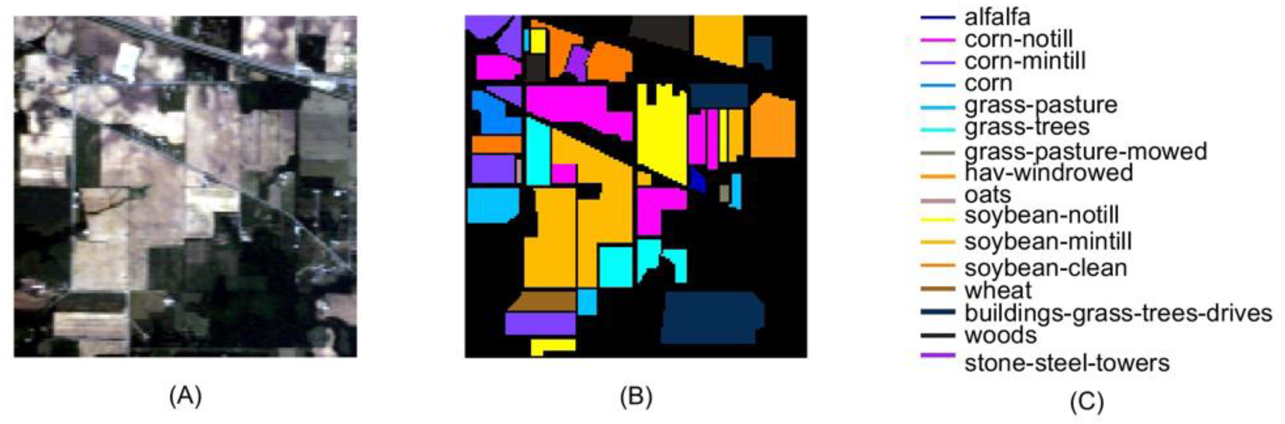
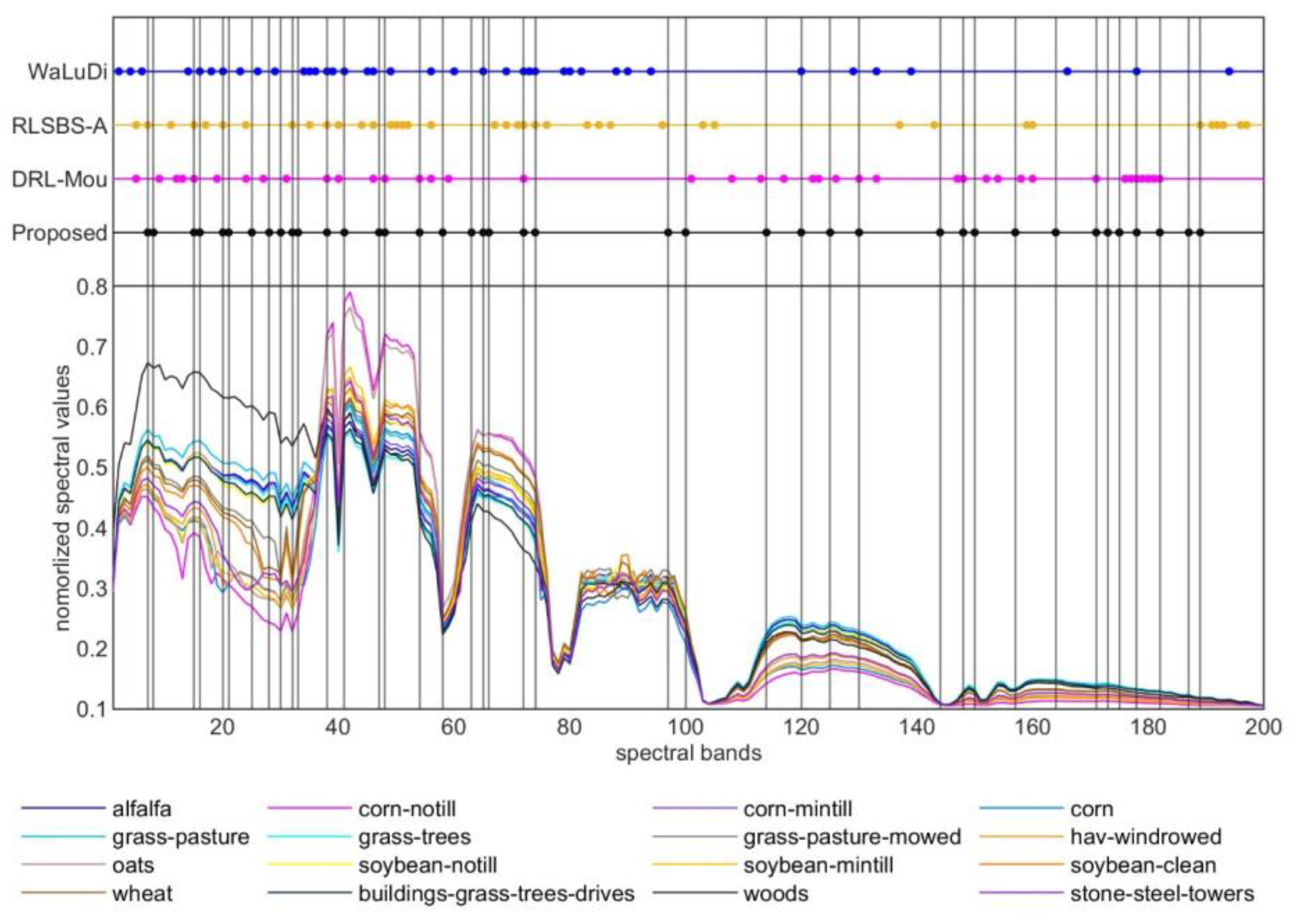
AVIRIS dataset: to validate the proposed BS method and compare it with other BS methods, a publicly available hyperspectral image dataset acquired using NASA’s Airborne Visible-Infrared Imaging Spectrometer sensor (AVIRIS) on 12 June 1992 was used. This particular dataset (the Indian Pines) was chosen because it has ground truth information captured through field observations and pixel-by-pixel labelled. It covers a geographical area in the northwest of Indiana in the United States as shown in Figure 2. The dataset includes 145 × 145 pixels, with pixel spatial resolution of 20 m. There are 220 bands in total, and the wavelength range is between 400–2500 nm. The data provided 16 types labelled data, most of which are crops and are they are in different growth stages. Before applying the BS methods, 20 bands (104–108, 150–163 and 220), all of which are water absorption bands, are removed. A total of 200 spectral bands are used as the input data.
(B)
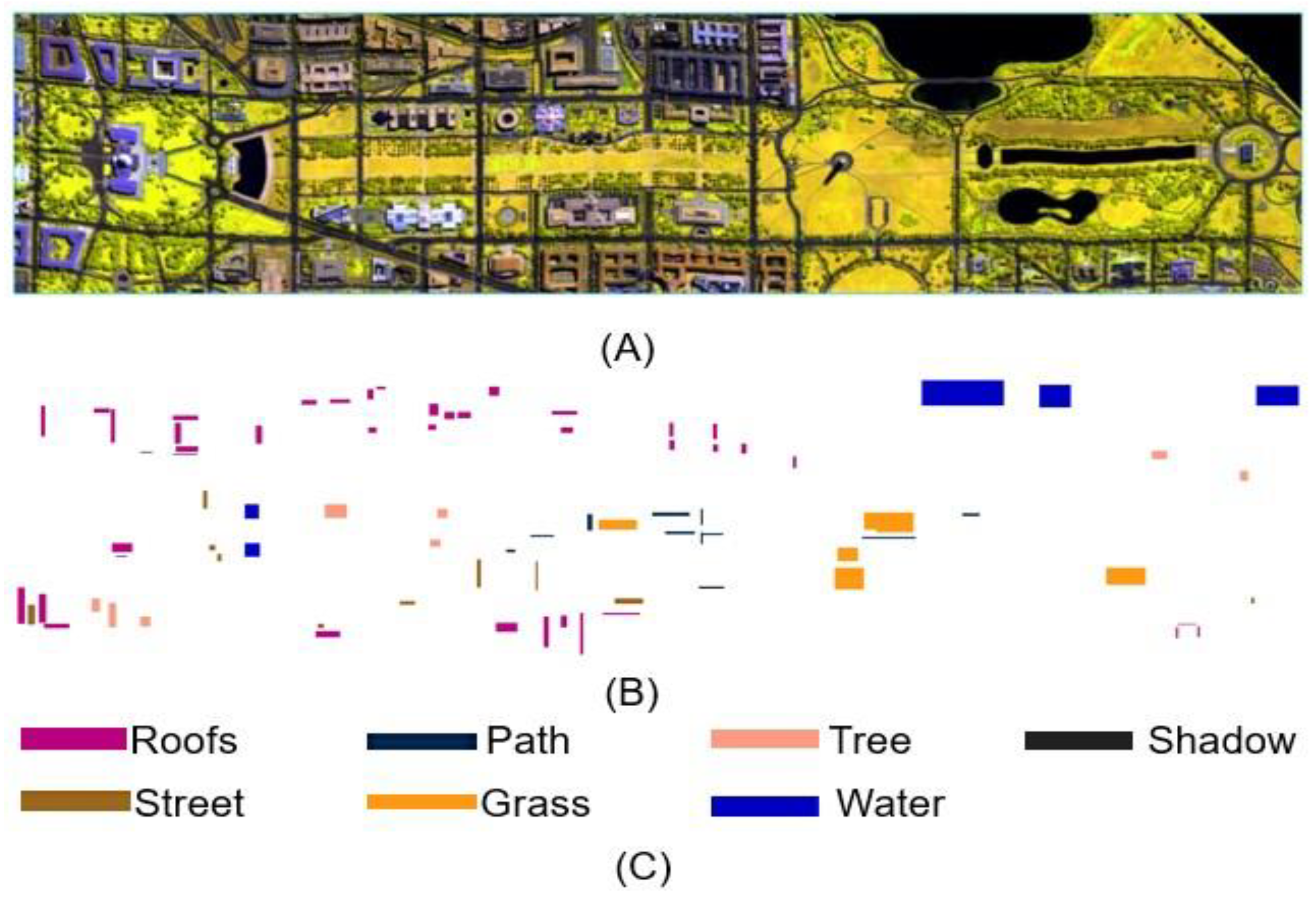
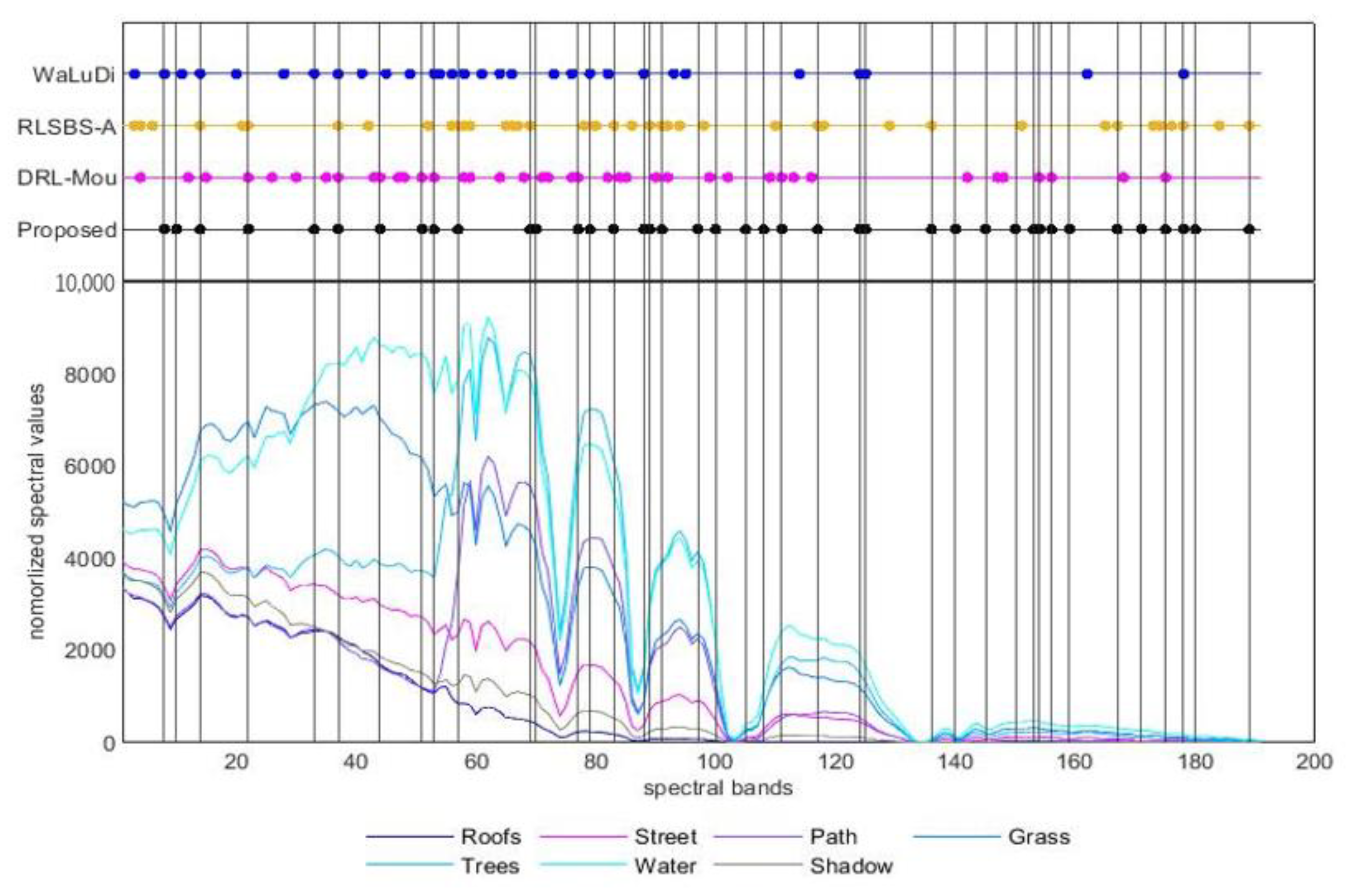
HYDICE dataset: the Washington District of Columbia (Washington DC) Mall dataset was captured using Hyperspectral Digital Imagery Collection Experiment (HYDICE) sensor over the urban region Washington DC Mall in 1995. HYDICE has 191 bands, and 0.4 µm to 2.4 µm spectral range. The image (only shows three bands), the ground truth and mapping classes are shown in Figure 3. This data set contains 1208 scan lines with 307 pixels in each scan line. It has seven classes (roofs, street, path, grass, trees, water, and shadow).
(C)
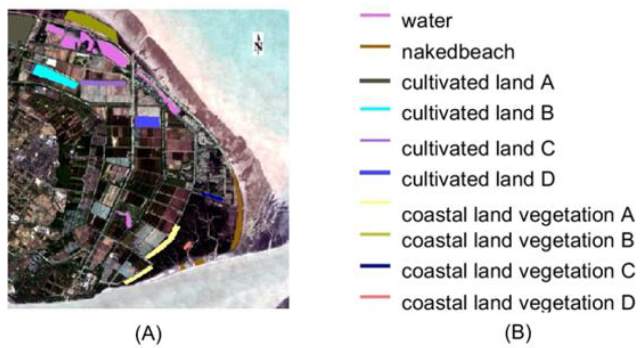
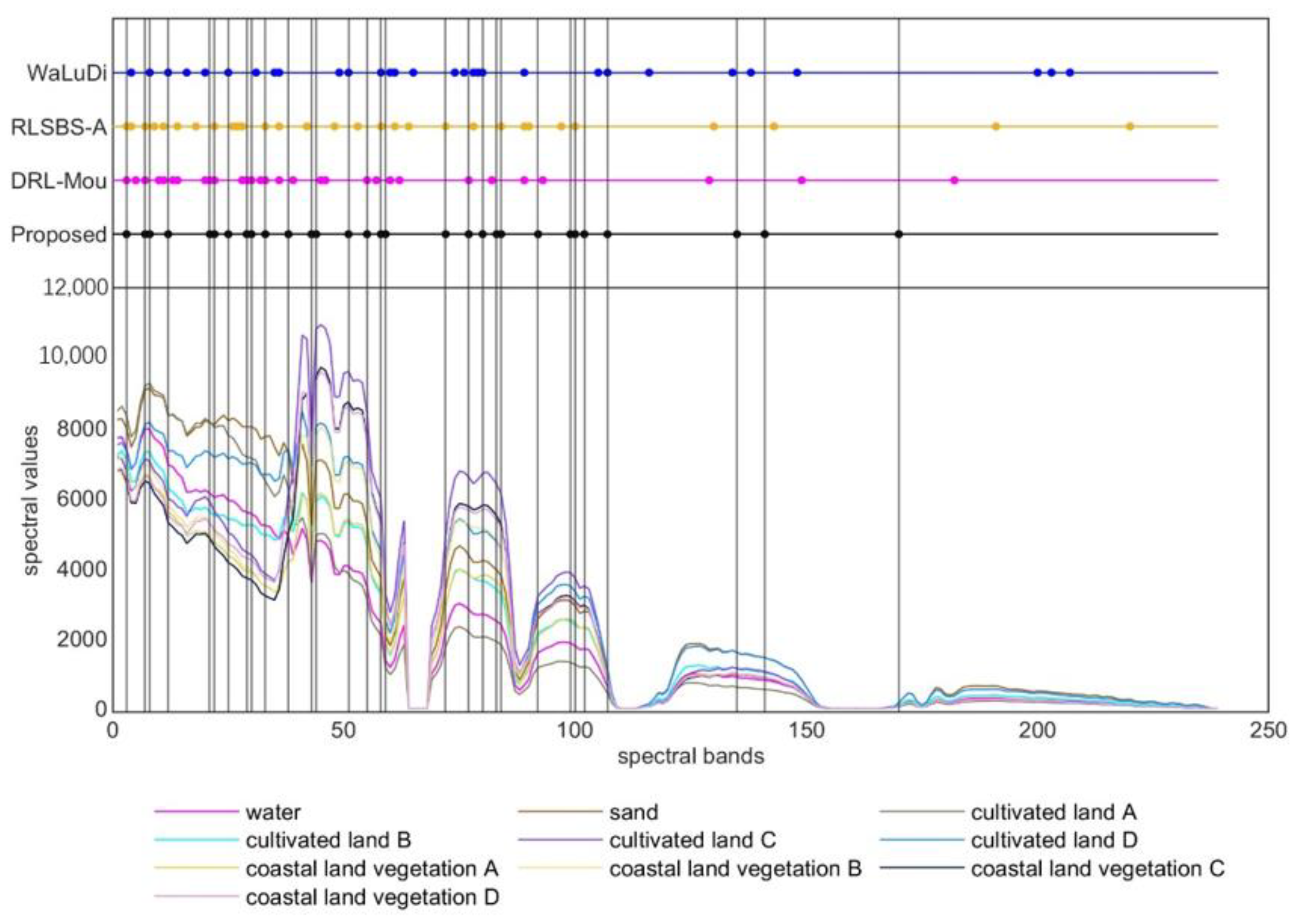
PRISMA dataset: PRISMA is a small satellite hyperspectral imaging sensor, managed and operated by the Italian Space Agency. It has a total of 239 spectral bands that acquire images at a 30 m spatial resolution and at a 10 nm spectral resolution. The entire hyperspectral range of bands in a PRISMA scene is from 400 nm to 2505 nm. Among 239 bands, 66 are in the visible and near infrared range (VNIR) and 173 are in the short-wave infrared range (SWIR). The Level 1 product was used for experiment. Chongming Island data from PRISMA was acquired on 8 May 2022. After evaluating Chongming Island PRISMA data, it was found that there are three empty bands in VNIR and 2 in SWIR. Ten types of common land cover types were manually sampled, including water body, bare sand, four types of coast bush vegetation, four types of cultivated land cover, there are 4775 sample pixels in total (Figure 4). The Indian Pines and Washington DC Mall datasets are from airborne hyperspectral sensors (ARIVIS and HYDICE, respectively). In order to further verify the performance of the proposed BS method, a recently available PRISMA satellite hyperspectral scene in a coast region (Chongming Island Shanghai China) was utilized.
(D)
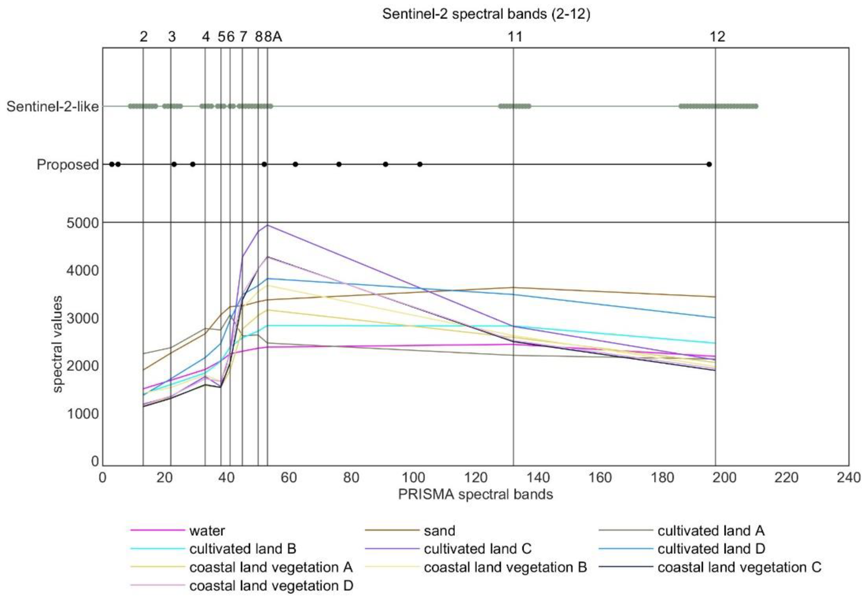
Sentinel-2 MRS: the Sentinel-2 multispectral data of Chongming Island was acquired at 02:35 (UTC time) on 8 May 2022 (by satellite Sentinel-2A), which is just 10 min apart from PRISMA data which was acquired at 02:45 (UTC time) on the same day, therefore it was a rare opportunity to compare hyperspectral and multispectral data performance on classification applications. Sentinel-2 is a high-resolution multispectral imaging satellite. The resolution of Bands 2, 3, 4, and 8 is 10 m. The resolution of bands 5, 6, 7, 8a, 11, and 12 is 20 m. In order to compare with PRISMA data, the Sentinel-2 data was resampled to 30 m. The corresponding band’s spectral range is as Table 1.

4. Experimental Design

Besides the proposed BS method (hereinafter abbreviated as proposed), the following three BS methods were implemented and conducted the experiments along with the proposed method:
(A)
PCA [11]: the most popular dimensionality reduction technology, which is widely used in many fields.
(B)
mvPCA [12]: a ranking-based BS method that uses an eigen analysis-based criterion to prioritize spectral bands.
(C)
ICA [14]: a method that compares mean absolute independent component analysis coefficients of individual spectral bands and picks independent ones including the maximum information. The stated three methods are feature extraction methods.
(D)
WaLuDi [37]: a BS method based on hierarchical clustering, which uses Kullback-Leibler divergence as the standard for clustering.
(E)
DRL-Mou [45]: a DRL (DQN based) BS method based on value function, also uses information entropy and/or band correlation as the reward function.
(F)
RLSBS-A [26]: a DRL (A3C based) BS method was used for BS, based on the mixture of policy and value function, also uses the loss function of the deep neural network based on semi-supervised classification as the reward function.
In order to analyze the performance of the proposed BS method and above-mentioned methods, the selected bands were fed into several classifiers to perform supervised classification tasks and the results were compared against the ground truth. The following classifiers were implemented: K-Near Neighbor algorithm (KNN) [51], n_neighbors is 2; Random Forest (RF) [52] (random_state is 20, n_estimators is 100); Support vector machine kernel radial basis function (SVM-RBF) [53]: based on radial basis function kernel, c = 100, kernel = ‘rbf’; Leave all settings of the algorithm on the default parameters of Scikit-learn [54]. CNN convolution neural network algorithm [26], which consists of a convolutional layer, pooled layer, and fully connected layer superimposed. In the multi-scale convolutional layer, the convolutional layer of 1 × 1 core is designed to extract spectral features, and the convolutional features of 3 × 3 nuclei are used to extract spatial features. After that, spatial and spectral features are cascaded and fed into the next layer. To speed up training, a batch normalization layer is added after evaluating each convolutional layer in the network.
The following criteria were used to validate the effectiveness of selected bands: the overall accuracy (OA), average accuracy assessments (AA) and kappa coefficient (Kappa). OA is calculated by summing the amount of correctly identified data and dividing by the total amount of data. AA is the average of each type of accuracy. Kappa coefficient is used to measure the consistency between the evaluation forecast and the ground truth (supplied labels).

5. Experimental Results

5.1. The Results of Reward Functions

For the Indian Pines dataset, three reward functions were compared: information entropy (IE), information gain (IG), and supervised reward (SR). In the proposed method, each of three reward functions was chosen as the reward function candidate to select bands. Then RF classifier was applied to these bands to perform the final classification tasks and the classification accuracy results were compared against the ground truth. The comparison results are shown in Figure 5. As can be seen in Figure 5, it clearly shows that as a reward function, IG performs better than other two reward functions in overall. Therefore, in the rest of experiments, IG was chosen as the reward function.
When the number of selected bands is 30, OA and Kappa have the high values and AA has the lowest values when IG was used as the reward function. Table 2 shows the confusion matrix, and Table 3 shows the accuracy of each type. The type number is the identifier of land cover which can be found in Figure 2C. In Table 2, sample number [6] represents the number of labeled samples of each type. The samples distribution is not uniform; the number of type 13–16 is not enough. Recognized number (RN) represents the recognized number of each type by the classifier. True Positive (TP) represents the number of correctly identified data of each type in RN. Accuracy represents the proportion of TP in RN. The last row in Table 3 shows the average accuracy of each type. 9323 is the total sample number of all labelled types. 7003 is the amount of correctly identified data in labelled types. 0.75 is the value of OA. It can be also found in Table 2 that the distribution of sample data is uneven. For type 15, the number of labelled samples is 23, the RF classifier recognized 20, 9 of them are correct, 11 of them are wrong. The accuracy of 0.45 ( 9 / 20 ) is low. The average accuracy is affected however for OA, 11 wrongly recognized samples have no significant effect on it.
It clearly shows that as a reward function, IG performs better than other two reward functions in overall. The OA and Kappa are more stable and important than AA. Therefore, in the rest of the experiments, IG was chosen as the reward function.

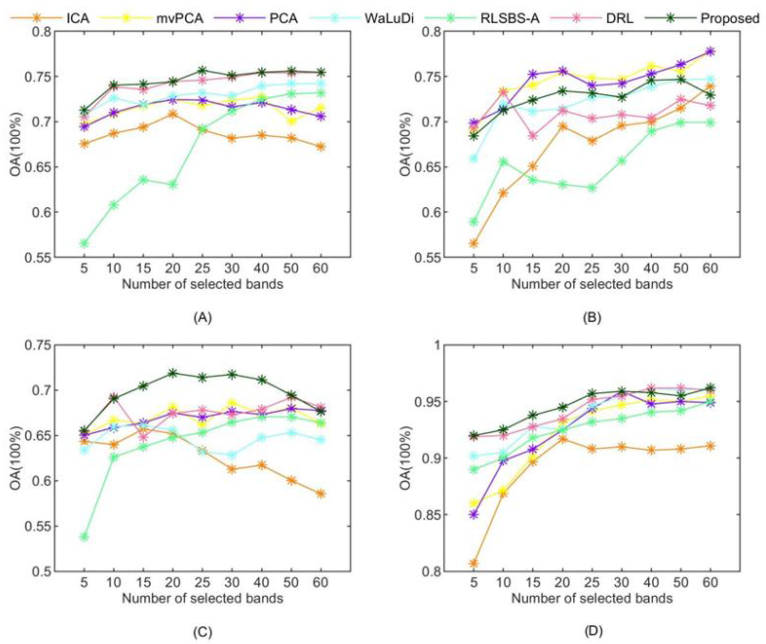
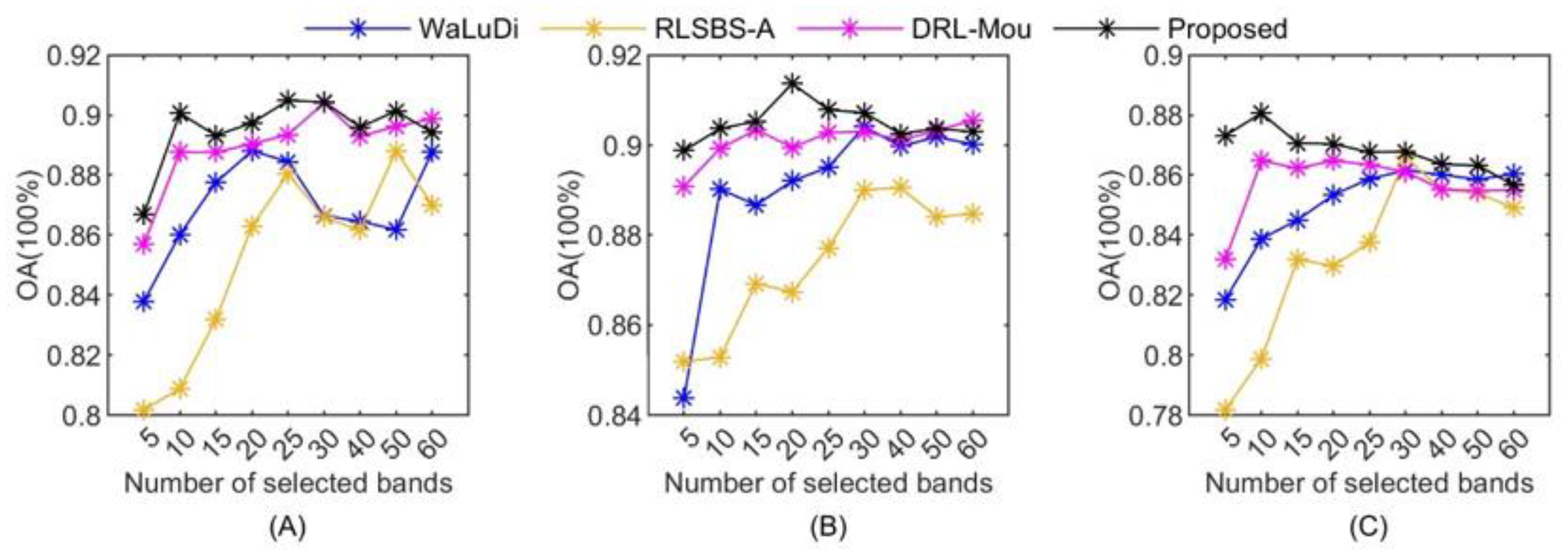
5.2. The Comparison of Different BS Methods

During the experiments, a various numbers of selected bands were conducted (K is the selected bands number). Figure 6 presents the results of each BS method with different numbers of bands (K) on the Indian Pines dataset. Table 4 shows the results when K is 40. The traditional machine learning algorithms (KNN, RF, SVM-RBF, CNN) were used as classifiers on the Indian Pines dataset. Table 5 shows the results of BS methods on Washington DC Mall dataset. Table 6 and Figure 7 show the result on Chongming dataset.
Excluding bands 1, 9, and 10 of Sentinel-2, the rest 10 bands of Sentinel-2 were used to conduct the classification using SVM-RBF as the classifier which got the best performance on PRISMA data. By applying the proposed BS method, 10 bands from PRISMA hyperspectral data were selected as is shown in Table 7. From Table 7, it can be seen that there are 3 selected PRISMA bands which are equivalent or very close to Sentinel-2’s. The final classification accuracies results were shown in Table 8. It is found that better classification accuracy can be derived from PRISMA data.
An extra task was performed to explore the PRISMA data further: to simulate Sentinel-2 bands using PRISMA data. Because there are usually several bands whose spectral ranges are within each Sentinel-2 band’s spectral range (see Figure 11 and Table 8), therefore a 10-band Sentinel-2-like data can be reconstructed from PRISMA using some techniques (averaging in our case). It is a very simple dimensionality reduction technique, and the classification accuracies using the simulated Sentinel-2-like PRISMA data is shown in Table 8. It is an interesting finding that through this simple dimensionality reduction technique, Sentinel-2-like PRISMA data outperformed Sentinel-2 and PRISMA band selected subset using the proposed method. Sentinel-2-like data has higher the signal-to-noise ratio, and the OA is higher. The results support the findings in [55].

6. Discussions

As can be seen in Figure 6, the proposed method has achieved the highest OA when RF, KNN, and CNN were used as the classifiers based on Indian Pines dataset. When K = 10 to 60, OA increased. The DRL-Mou method has the same trends as the proposed method. For the purpose of dimensionality reduction, the number of the selected bands should not be too big or too small, considering the uneven distributed sample data which results the decrease in AA, after conducting many tests, a reasonable number of the selected band is set to 40 (K = 40) which seems representing the hyperspectral data quite well.
As shown in Table 4, in the deep convolution neural network algorithm (CNN), the bands selected by all methods are more than 90% in the classification. Except ICA, the accuracy is about 95%. This paper randomly intercepts continuous bands for classification, such as 1–40 bands, which can also reach 95% by using CNN classification. Experiments show that if the depth neural network algorithm is used for ground object classification, the band selection is not necessary. Another reason that all SB methods have high OA is that if the small data sample is used for classification in the deep neural network, it is likely to be over fitted. Therefore, the else experiments did not use the CNN for justify.
DRL methods (the proposed one or DRL-Mou and RLSBS-A methods) are better than clustering method (WaLuDi). The proposed method can achieve the highest OA when using RF, SVM-RBF and KNN are used as the classifiers. Although the AA of proposed method is a little bit lower than that of clustering methods while RF was employed as the classifier. Compared with the other two reinforcement learning methods (DRL-Mou and RLSBS-A), the proposed method performed better, the main reason is that the proposed method has better “supervised” when the labelled data is introduced into the reward mechanism. Among all BS models, the feature extraction methods such as PCA, mvPCA perform instable in classification, and the ICA method performs relatively poor. Deep learning algorithm tends to achieve good results in classification, but it is not applicable to evaluation BS.
The Washington DC Mall dataset (HYDICE sensor) has distinct spectral characteristics in land covers comparing to the Indian Pines dataset (AVIRIS sensor). Therefore, the classification task is relatively easy for all BS methods when they are applied to the Washington DC Mall dataset, the classification accuracies of all methods are high (96% or above), as shown in Table 5. However, the proposed BS method can still be considered the best performer in overall.
Table 6 presents accuracy assessments on the band selection results from Chongming Island PRISMA dataset. mvPCA and PCA have more higher OA using RF classifier with 10 to 60 selected bands than the proposed method. The PCA and mvPCA is much better than other methods on KNN and RF, but there is only less than 2 percentage point difference between the proposed method and feature extraction on RF. They all more than 90%; while among DRL based BS methods, the proposed method performed much better than the other two DRL based BS methods. The proposed method achieved the highest OA when using RF, SVM-RBF and KNN as the classifiers. Assessing the PRISMA data, K = 30 was chosen. The results when K = 30 is shown in Table 6.
Overall, it can be seen that among all band selection models, the feature extraction methods such as PCA, mvPCA had instable performances, and the ICA method’s performance was relatively poor. The proposed method performed very well in all cases. Deep learning algorithm tended to achieve good results in classification, but it was not applicable to evaluate band selection.
In order to visualize which bands were selected, all bands selected by different methods were located on the spectral curves. The selected bands’ locations on the spectral curves can be found in Figure 8, Figure 9, Figure 10 and Figure 11. It can be seen that for most BS methods, the most of the selected bands are in the range of near-infrared bands. Comparing to other BS methods, the proposed method tends to select bands at the turning points on the spectral curves and the selected bands are evenly distributed across the spectral range. In other words, the proposed method can capture the most significant bands (spectral characteristics) better than others therefore the resultant selected bands present the original hyperspectral data better. It is evidenced by the accuracy assessments.
Figure 8. Forty selected bands’ locations which are represented with dots on spectral curves by different BS methods for the Indian Pines dataset.
Remotesensing 15 00682 g008
Figure 9. Thirty selected bands’ locations which are represented with dots on spectral curves by different BS methods for the Washington DC Mall dataset.
Remotesensing 15 00682 g009
Figure 10. Thirty elected bands’ locations which are represented with dots on spectral by different BS methods for Chongming Island PRISMA dataset.
Remotesensing 15 00682 g010
Figure 11. Visualization of selected bands and bands’ locations of Chongming Island PRISMA and Sentinel-2 dataset.
Remotesensing 15 00682 g011

7. Conclusions

In this paper, a partially supervised deep reinforcement learning method for hyperspectral band selection is proposed. This proposed method uses labeled data to optimize the reward scheme and makes reinforcement learning supervised. The proposed method was applied in classification applications using both airborne and spaceborne hyperspectral data. The experiment results demonstrated that the further improvements could be achieved using the proposed method comparing to other similar band selection methods. Another advantage of the proposed method is that it tends to choose the most spectral significant bands and the chosen bands are well distributed along the spectral dynamic range, therefore the resultant bands present the original hyperspectral data better.
The experimental datasets include three types of areas: farms, towns, and coastal areas. The more complex and difficult to distinguish the land cover the data is, the more suitable for band selection the data becomes. The data with good discrimination, such as towns, each method has a high score on OA and AA, for BS method is not obvious. In the future the proposed band selection method will focus on more complex land covers using hyperspectral data.
The proposed method provides a new deep reinforcement learning method for hyperspectral band selection. In addition to classification tasks, it can be easily extended to other tasks such as target detection, semantic segmentation, and the other decision-making applications. Those are the future research areas that the authors are going to explore.

Author Contributions

H.Y.: conceptualization, methodology, investigation, experiment analysis, writing—original draft; M.C.: conceptualization, supervision, writing—review and editing; G.W.: conceptualization, methodology; J.W.: data curation, review and editing; Y.W.: visualization, review and editing; Z.H.: review and editing. All authors have read and agreed to the published version of the manuscript.

Funding

This study was funded by Shanghai Science and Technology Innovation Action Planning, No.20dz1203800.

Data Availability Statement

The original contributions presented in the study are public evaluation data and free satellite data, further inquiries can be directed to the corresponding author.

Acknowledgments

The authors gratefully acknowledge the following organizations for providing the experimental datasets: Purdue Research Foundation, ESA (European Space Agency) and ASI (Italian Space Agency) for providing AVIRIS/HYDICE, Sentinel-2 and PRISMA datasets, respectively. We also thank authors of papers [26,45] for making their code available which enables our comparison study.

Conflicts of Interest

The authors declare that the research was conducted in the absence of any commercial or financial relationships that could be construed as a potential conflict of interest.

References

  1. Yan, Y.; Liying, L.; Wang’e, X. Mechanical Structure Design for Hyperspectral Imager of HJ-1A Satellite. Spacecr. Eng. 2009, 18, 97–105. [Google Scholar]
  2. Zhan, H. The First Two Satellites OVS-1A/1B of Zhuhai-1 Remote-sensing Micro/Nano Satellites Constellation Launched Successfully. Space Int. 2017, 462, 1674–9030. [Google Scholar]
  3. Shanshan, M. Gaofen 5 and Gaofen 6 Satellites Put into Operation. Aerosp. China 2019, 20, 58. [Google Scholar]
  4. Kerr, G.; Avbelj, J.; Carmona, E.; Eckardt, A.; Gerasch, B.; Graham, L.; Günther, B.; Heiden, U.; Krutz, D.; Krawczyk, H.; et al. The hyperspectral sensor DESIS on MUSES: Processing and applications. In Proceedings of the 2016 IEEE International Geoscience and Remote Sensing Symposium (IGARSS), Beijing, China, 10–15 July 2016; pp. 268–271. [Google Scholar]
  5. Pignatti, S.; Palombo, A.; Pascucci, S.; Romano, F.; Santini, F.; Simoniello, T.; Umberto, A.; Vincenzo, C.; Acito, N.; Diani, M.; et al. The PRISMA hyperspectral mission: Science activities and opportunities for agriculture and land monitoring. In Proceedings of the 2013 IEEE International Geoscience and Remote Sensing Symposium-IGARSS, Melbourne, VIC, Australia, 21–26 July 2013; pp. 4558–4561. [Google Scholar]
  6. Guanter, L.; Kaufmann, H.; Segl, K.; Foerster, S.; Rogass, C.; Chabrillat, S.; Küster, T.; Hollstein, A.; Rossner, G.; Chlebek, C.; et al. The EnMAP Spaceborne Imaging Spectroscopy Mission for Earth Observation. Remote Sens. 2015, 7, 8830–8857. [Google Scholar] [CrossRef] [Green Version]
  7. Landgrebe, D. Hyperspectral image data analysis. IEEE Signal Process. Mag. 2002, 19, 17–28. [Google Scholar] [CrossRef]
  8. Chang, C.-I.; Wang, S. Constrained band selection for hyperspectral imagery. IEEE Trans. Geosci. Remote Sens. 2006, 44, 1575–1585. [Google Scholar] [CrossRef]
  9. Jimenez-Rodriguez, L.O.; Arzuaga-Cruz, E.; Velez-Reyes, M. Unsupervised Linear Feature-Extraction Methods and Their Effects in the Classification of High-Dimensional Data. IEEE Trans. Geosci. Remote Sens. 2007, 45, 469–483. [Google Scholar] [CrossRef]
  10. Jimenez, L.O.; Landgrebe, D.A. Supervised classification in high-dimensional space: Geometrical, statistical, and asymptotical properties of multivariate data. IEEE Trans. Syst. Man Cybern. Part C 1998, 28, 39–54. [Google Scholar] [CrossRef]
  11. Elghazawi, T.; Kaewpijit, S.; Moigne, J.L. Parallel and Adaptive Reduction of Hyperspectral Data to Intrinsic Dimensionality. IEEE Int. Conf. Clust. Comput. 2001, 107, 215–224. [Google Scholar]
  12. Chang, C.I.; Qian, D.; Sun, T.L.; Althouse, M.L.G. A joint band prioritization and band-decorrelation approach to band selection for hyperspectral image classification. IEEE Trans. Geosci. Remote Sens. 1999, 37, 2631–2641. [Google Scholar] [CrossRef] [Green Version]
  13. Bruce, L.M.; Koger, C.H. Dimensionality reduction of hyperspectral data using discrete wavelet transform feature extraction. IEEE Trans. Geosci. Remote Sens. 2002, 40, 2331–2338. [Google Scholar] [CrossRef]
  14. Lennon, M.; Mercier, G.; Mouchot, M.-C.; Hubert-Moy, L. Independent component analysis as a tool for the dimensionality reduction and the representation of hyperspectral images. In Proceedings of the IGARSS 2001. Scanning the Present and Resolving the Future. Proceedings. IEEE 2001 International Geoscience and Remote Sensing Symposium (Cat. No.01CH37217), Sydney, NSW, Australia, 9–13 July 2001; Volume 6, pp. 2893–2895. [Google Scholar] [CrossRef] [Green Version]
  15. Maji, B.; Swain, M. Advanced Fusion-Based Speech Emotion Recognition System Using a Dual-Attention Mechanism with Conv-Caps and Bi-GRU Features. Electronics 2022, 22, 1328. [Google Scholar] [CrossRef]
  16. Bruzzone, L. An extension of the Jeffreys-Matusita distance to multiclass cases for feature selection. IEEE Trans. Geosci. Remote Sens. 1995, 33, 1318–1321. [Google Scholar] [CrossRef]
  17. Serpico, S.B.; Bruzzone, L. A new search algorithm for feature selection in hyperspectral remote sensing images. IEEE Trans. Geosci. Remote Sens. 2001, 39, 1360–1367. [Google Scholar] [CrossRef]
  18. Yang, H.; Du, Q.; Su, H.; Sheng, Y. An Efficient Method for Supervised Hyperspectral Band Selection. IEEE Geosci. Remote Sens. Lett. 2011, 8, 138–142. [Google Scholar] [CrossRef]
  19. Cao, X.; Tao, X.; Jiao, L. Supervised Band Selection Using Local Spatial Information for Hyperspectral Image. IEEE Geosci. Remote Sens. Lett. 2016, 13, 329–333. [Google Scholar] [CrossRef]
  20. Tang, Y.; Fan, E.; Yan, C.; Bai, X.; Zhou, J. Discriminative weighted band selection via one-class SVM for hyperspectral imagery. In Proceedings of the 2016 IEEE International Geoscience and Remote Sensing Symposium (IGARSS), Beijing, China, 10–15 July 2016; pp. 2765–2768. [Google Scholar] [CrossRef] [Green Version]
  21. Feng, S.; Itoh, Y.; Parente, M.; Duarte, M.F. Hyperspectral Band Selection From Statistical Wavelet Models. IEEE Trans. Geosci. Remote Sens. 2017, 55, 2111–2123. [Google Scholar] [CrossRef]
  22. Li, H.; Wang, Y.; Duan, J.; Xiang, S.; Pan, C. Group sparsity based semi-supervised band selection for hyperspectral images. In Proceedings of the 2013 IEEE International Conference on Image Processing, Melbourne, VIC, Australia, 15–18 September 2013; pp. 3225–3229. [Google Scholar]
  23. Feng, J.; Jiao, L.; Liu, F.; Sun, T.; Zhang, X. Mutual-Information-Based Semi-Supervised Hyperspectral Band Selection with High Discrimination, High Information, and Low Redundancy. IEEE Trans. Geosci. Remote Sens. 2015, 53, 2956–2969. [Google Scholar] [CrossRef]
  24. Guo, Z.; Xiao, B.; Zhang, Z.; Zhou, J. A hypergraph based semi-supervised band selection method for hyperspectral image classification. In Proceedings of the 2013 IEEE International Conference on Image Processing, Melbourne, VIC, Australia, 15–18 September 2013. [Google Scholar]
  25. Su, H.; Yong, B.; Qian, D. Hyperspectral Band Selection Using Improved Firefly Algorithm. IEEE Geosci. Remote Sens. Lett. 2015, 13, 68–72. [Google Scholar] [CrossRef]
  26. Feng, J.; Li, D.; Gu, J.; Cao, X.; Jiao, L. Deep Reinforcement Learning for Semisupervised Hyperspectral Band Selection. IEEE Trans. Geosci. Remote Sens. 2021, 60, 1–19. [Google Scholar] [CrossRef]
  27. Sui, C.; Yan, T.; Xu, Y.; Yong, X. Unsupervised Band Selection by Integrating the Overall Accuracy and Redundancy. IEEE Geosci. Remote Sens. Lett. 2015, 12, 185–189. [Google Scholar]
  28. Zhang, M.; Ma, J.; Gong, M. Unsupervised Hyperspectral Band Selection by Fuzzy Clustering with Particle Swarm Optimization. IEEE Geosci. Remote Sens. Lett. 2017, 14, 773–777. [Google Scholar] [CrossRef]
  29. Chang, C. Hyperspectral Data Exploitation: Theory and Applications; John Wiley & Sons: Hoboken, NJ, USA, 2007. [Google Scholar]
  30. Guo, B.; Gunn, S.R.; Damper, R.I.; Nelson, J. Band Selection for Hyperspectral Image Classification Using Mutual Information. IEEE Geosci. Remote Sens. Lett. 2006, 3, 522–526. [Google Scholar] [CrossRef]
  31. Jia, S.; Tang, G.; Zhu, J.; Li, Q. A Novel Ranking-Based Clustering Approach for Hyperspectral Band Selection. IEEE Trans. Geosci. Remote Sens. 2016, 54, 88–102. [Google Scholar] [CrossRef]
  32. Wang, Q.; Zhang, F.; Li, X. Optimal Clustering Framework for Hyperspectral Band Selection. IEEE Trans. Geosci. Remote Sens. 2018, 56, 5910–5922. [Google Scholar] [CrossRef] [Green Version]
  33. Qian, Y.; Yao, F.; Jia, S. Band selection for hyperspectral imagery using affinity propagation. IET Comput. Vis. 2008, 3, 213–222. [Google Scholar] [CrossRef]
  34. Sun, K.; Geng, X.; Ji, L. Exemplar Component Analysis: A Fast Band Selection Method for Hyperspectral Imagery. IEEE Geosci. Remote Sens. Lett. 2015, 12, 998–1002. [Google Scholar]
  35. Ahmad, M.; Haq, I.U.; Mushtaq, Q.; Sohaib, M. A New Statistical Approach for Band Clustering and Band Selection Using K-Means Clustering. Int. J. Eng. Technol. 2011, 3, 606–614. [Google Scholar]
  36. Ding, Y.; Yuan, X.; Di, Z.; Dong, L.; An, Z. Feature representation and selection in malicious code detection methods based on static system calls. Comput. Secur. 2011, 30, 514–524. [Google Scholar]
  37. Martinez-Uso, A.; Pla, F.; Sotoca, J.M.; García-Sevilla, P. Clustering-Based Hyperspectral Band Selection Using Information Measures. IEEE Trans. Geosci. Remote Sens. 2007, 45, 4158–4171. [Google Scholar] [CrossRef]
  38. Duan, P.; Kang, X.; Li, S.; Ghamisi, P. Multichannel Pulse-Coupled Neural Network-Based Hyperspectral Image Visualization. IEEE Trans. Geosci. Remote Sens. 2019, 58, 2444–2456. [Google Scholar] [CrossRef]
  39. Li, S.; Song, W.; Fang, L.; Chen, Y.; Ghamisi, P.; Benediktsson, J.A. Deep Learning for Hyperspectral Image Classification: An Overview. IEEE Trans. Geosci. Remote Sens. 2019, 57, 6690–6709. [Google Scholar] [CrossRef] [Green Version]
  40. Wang, Q.; Li, Q.; Li, X. Hyperspectral Band Selection via Adaptive Subspace Partition Strategy. IEEE J. Sel. Top. Appl. Earth Obs. Remote Sens. 2019, 12, 4940–4950. [Google Scholar] [CrossRef]
  41. Roy, S.K.; Chatterjee, S.; Bhattacharyya, S.; Chaudhuri, B.B.; Platos, J. Lightweight Spectral-Spatial Squeeze-and-Excitation Residual Bag-of-Features Learning for Hyperspectral Classification. IEEE Trans. Geosci. Remote Sens. 2020, 58, 5277–5290. [Google Scholar] [CrossRef]
  42. Hu, J.; Shen, L.; Sun, G. Squeeze-and-Excitation Networks. IEEE Trans. Pattern Anal. Mach. Intell. 2017, 7132–7141. [Google Scholar] [CrossRef] [Green Version]
  43. Fu, J.; Liu, J.; Tian, H.; Li, Y.; Bao, Y.; Fang, Z.; Lu, H. Dual Attention Network for Scene Segmentation. In Proceedings of the 2019 IEEE/CVF Conference on Computer Vision and Pattern Recognition (CVPR), Long Beach, CA, USA, 15–20 June 2019; pp. 3141–3149. [Google Scholar]
  44. Cai, Y.; Liu, X. BS-Nets: An End-to-End Framework for Band Selection of Hyperspectral Image. IEEE Trans. Geosci. Remote Sens. 2020, 58, 1969–1984. [Google Scholar] [CrossRef]
  45. Mou, L.; Saha, S.; Hua, Y.; Bovolo, F.; Bruzzone, L.; Zhu, X.X. Deep Reinforcement Learning for Band Selection in Hyperspectral Image Classification. IEEE Trans. Geosci. Remote Sens. 2022, 60, 1–14. [Google Scholar] [CrossRef]
  46. Arulkumaran, K.; Deisenroth, M.P.; Brundage, M.; Bharath, A.A. Deep reinforcement learning: A brief survey. IEEE Signal Process. Mag. 2017, 34, 26–38. [Google Scholar] [CrossRef] [Green Version]
  47. Krizhevsky, A.; Sutskever, I.; Hinton, G.E. ImageNet classification with deep convolutional neural networks. Commun. ACM 2012, 60, 84–90. [Google Scholar] [CrossRef] [Green Version]
  48. Mnih, V.; Kavukcuoglu, K.; Silver, D.; Graves, A.; Antonoglou, I.; Wierstra, D.; Riedmiller, M.A. Playing Atari with Deep Reinforcement Learning. arXiv 2013, arXiv:1312.5602. [Google Scholar]
  49. Van Hasselt, H. Double Q-learning. In Advances in Neural Information Processing Systems 23 (NIPS 2010), Proceedings of the 24th Annual Conference on Neural Information Processing Systems 2010, Vancouver, BC, Canada, 6–9 December 2010; Curran Associates, Inc.: Red Hook, NY, USA, 2010; pp. 2613–2621. [Google Scholar]
  50. Hasselt, H.V.; Guez, A.; Silver, D. Deep Reinforcement Learning with Double Q-learning. arXiv 2015, arXiv:1509.06461. [Google Scholar] [CrossRef]
  51. Hellman, M.E. The Nearest Neighbor Classification Rule with a Reject Option. IEEE Trans. Syst. Sci. Cybern. 1970, 6, 179–185. [Google Scholar] [CrossRef]
  52. Breiman, L. Random Forests. Mach. Learn. 2001, 45, 5–32. [Google Scholar] [CrossRef] [Green Version]
  53. Hearst, M.A.; Dumais, S.T.; Osman, E.; Platt, J.; Scholkopf, B. Support vector machines. IEEE Intell. Syst. Appl. 1998, 13, 18–28. [Google Scholar] [CrossRef] [Green Version]
  54. Swami, A.; Jain, R. Scikit-learn: Machine Learning in Python. J. Mach. Learn. Res. 2013, 12, 2825–2830. [Google Scholar]
  55. Jia, J.; Chen, J.; Zheng, X.; Wang, Y.; Guo, S.; Sun, H.; Jiang, C.; Karjalainen, M.; Karila, K.; Duan, Z.; et al. Tradeoffs in the Spatial and Spectral Resolution of Airborne Hyperspectral Imaging Systems: A Crop Identification Case Study. IEEE Trans. Geosci. Remote Sens. 2022, 60, 1–18. [Google Scholar] [CrossRef]
Figure 1. An overview of DDQN model for hyperspectral band selection. In the training phase, Q-network interacts with a tailored reword function in order to learn a band-selection policy by trial and error. In the test phase, the method selects bands according to the learned policy.
Remotesensing 15 00682 g001
Figure 2. The dataset of the Indian Pines from AVIRIS airborne hyperspectral sensor: (A) is the Indian Pines three-band display image using bands 30, 20 and 10 as red green and blue channels; (B) is the Indian Pines land cover map (ground truth); (C) is the color and name for each Indian Pines land cover.
Remotesensing 15 00682 g002
Figure 3. The dataset of the Washington DC Mall from HYDICE airborne hyperspectral sensor: (A) is the Washington DC Mall three-band display image using bands 90, 69 and 7; (B) is the Washington DC Mall ground truth image that the position corresponds to (A); (C) is the color and name for each Washington DC Mall land cover (ground truth).
Remotesensing 15 00682 g003
Figure 4. The Chongming Island PRISMA dataset: (A) PRISMA image displayed as RGB with bands of 31, 20 and 10, respectively, PRISMA data was acquired 02:45 (UTC) on 8 May 2022; (B) the color-coded land cover classes.
Remotesensing 15 00682 g004
Figure 5. Classification accuracy comparisons when three different reward functions were used in the proposed BS method: (A) OA results under various numbers of selected bands; (B) AA results under various numbers of selected bands; (C) Kappa results under various numbers of selected bands.
Remotesensing 15 00682 g005
Figure 6. OA results of different BS methods for the Indian Pines dataset: (A) using RF as the classifier; (B) using SVM-RBF as the classifier; (C) using KNN as the classifier; (D) using CNN as the classifier.
Remotesensing 15 00682 g006
Figure 7. OA results of different BS methods for Chongming Island PRISMA dataset: (A) using RF as the classifier; (B) using SVM-RBF as the classifier; (C) using KNN as the classifier.
Remotesensing 15 00682 g007
Table 1. Band comparison between Chongming Island PRISMA and Sentinel-2 datasets.
Sentinel-2 BandCenter WavelengthBandwidthPRISMA Bands
1-Coastal aerosol442.3215–8
2-Blue492.1669–17
3-Green5593620–25
4-Red6653132–35
5-Vegetation red edge703.81637–39
6-Vegetation red edge739.11541–42
7-Vegetation red edge779.72044–46
8-NIR83310647–52
8A-Narrow NIR8642253–54
9-Water vapour9432160–61
10-SWIR-Cirrus1376.930109–112
11-SWIR1610.494128–137
12-SWIR2185.7185186–209
Table 2. The confusion matrix obtained by the proposed method using RF classifier, 30 bands were selected by using IG as the reward function.
Types12345678910111213141516SN
1888197260822552600410001290
2115369160208187530000000750
3621458350430320010010210
4021366121052203660140447
5000965101010280000672
6000514320000010100440
74360231540241300000041871
810630081538719214300600112221
990311512126942870004010552
100000501001640200000190
110002070000111043200001164
120001187000015961311001342
1301000021020016900085
1400050281400000100048
150002012000000009023
160000120000002000418
RN1304472974348084877572744476180123821275122079323
TP88836958366651432540192128716411041316910947003
accuracy0.680.780.600.840.810.890.710.700.600.910.890.620.920.830.450.570.75(OA)
Table 3. The classification average accuracy assessments (AA) of three reward functions. The proposed BS method was used for the Indian Pines dataset and the selected band number was set to 30.
TypeIEIGSR
10.670.680.67
20.770.780.76
30.610.600.62
40.860.840.86
50.810.810.79
60.870.890.88
70.700.710.71
80.700.700.70
90.580.600.57
100.900.910.89
110.900.890.89
120.620.620.55
130.920.920.96
140.880.830.75
150.800.451.00
160.670.570.67
AA0.770.740.77
Table 4. Comparisons different BS methods for the Indian Pines dataset with 40 selected bands. The first row indicates the classification assessment criteria (OA, AA, and Kappa) when different classifiers were used, the first column lists the BS methods.
ClassifiersKNNRFSVM-RBFCNN
BSOAAAKappaOAAAKappaOAAAKappaOAAAKappa
PCA0.67310.65360.62720.72120.74300.67640.75270.73930.71720.94780.91780.9328
mvPCA0.67340.64090.62830.72750.71420.68410.76160.75250.72700.95170.90270.9422
ICA0.61710.58390.56220.68510.70190.63340.69970.69860.65430.90690.84210.9226
WaLuDi0.64740.61020.59800.73960.77600.69950.73900.73710.71180.96190.93230.9565
RLSBS-A0.67070.65370.62500.72490.78390.68200.68960.68490.63910.94060.86210.9322
DRL-Mou0.67900.66880.63380.75420.76570.71670.70420.63880.65650.96170.91540.9563
Proposed0.71140.68280.67040.75470.77330.71760.74570.74280.70410.95780.91380.9518
Table 5. Comparisons different BS methods for the Washington DC Mall dataset with 30 selected bands. The first row indicates the classification assessment criteria (OA, AA, and Kappa) when different classifiers were used, the first column lists the BS methods.
ClassifiersKNNRFSVM-RBF
BSOAAAKappaOAAAKappaOAAAKappa
PCA0.98420.96850.97940.98450.97460.97970.98570.97510.9813
mvPCA0.98150.92420.96930.98200.96500.93550.98320.96600.9799
WaLuDi0.97220.96280.97670.97720.95670.97010.97300.96500.9778
RLSBS-A0.98430.96470.97950.98350.96560.97850.98310.96620.9778
DRL-Mou0.98380.95060.97880.98330.96340.97810.98350.97250.9785
Proposed0.98500.98040.96550.98370.95630.97870.98570.97630.9812
Table 6. Comparisons different BS methods on the PRISMA dataset with 30 selected bands. The first row indicates the classification assessment criteria (OA, AA, and Kappa) when different classifiers were used, the first column lists BS methods.
ClassifiersKNNRFSVM-RBF
BSOAAAKappaOAAAKappaOAAAKappa
PCA0.85180.85730.83460.90720.91550.89630.73250.77900.7172
mvPCA0.85810.86300.84170.91510.92270.90520.63480.69260.6259
WaLuDi0.84360.85260.82550.86460.85260.84880.89970.90530.8880
RlSBS-A0.82740.83280.80740.88040.90130.88490.88690.88890.8738
DRL-Mou0.86110.86460.84500.90490.91050.89530.90300.91020.8917
Proposed0.86780.87150.85260.90440.90940.89320.90720.91400.8964
Table 7. The PRISMA bands selected using the proposed method.
PRISMA Band35232952627691102195
Center Wavelength (nm)4194345716238559621008116312842175
Sentinel-2 band 3 8 12
Table 8. Comparisons of classification accuracies between hyperspectral data PRISMA and multispectral data Sentinel-2 of Chongming Island. Only 10 selected bands (by the proposed method) from PRISMA were used. The Sentinel-2-like is the 10 Sentinel-2 like 10 bands reconstructed from PRISMA.
OAAAKappa
Sentinel-2 (10 bands)0.87550.87870.8610
PRISMA (10 selected bands)0.90370.91080.8925
Sentinel-2-like (10 simulated bands)0.97020.97000.9668
Disclaimer/Publisher’s Note: The statements, opinions and data contained in all publications are solely those of the individual author(s) and contributor(s) and not of MDPI and/or the editor(s). MDPI and/or the editor(s) disclaim responsibility for any injury to people or property resulting from any ideas, methods, instructions or products referred to in the content.

