High-Rate One-Hourly Updated Ultra-Rapid Multi-GNSS Satellite Clock Offsets Estimation and Its Application in Real-Time Precise Point Positioning

Abstract

The requirement of timeliness is increasing while obtaining precise tempo-spatial information with the development of global navigation satellite systems (GNSSs). Due to the poor network environment and communication conditions in some regions or application scenarios, it is difficult for users to receive real-time (RT) precise products. The hourly updated ultra-rapid products with low latency and high accuracy are of great interest in GNSS real-time and near-real-time fields. However, it is difficult to achieve the high-rate one-hourly updated precise clock estimation (PCE); since many ambiguity parameters need to be estimated, the computation is time-consuming. At present, the highest time resolution of ultra-rapid clock offsets is 15 min. The low samplings affect the prediction accuracy of clock offsets and the precise point positioning (PPP) performances. To meet these requirements, we proposed an efficient method and design a new framework for high-rate one-hourly updated ultra-rapid PCE. We modified the epoch-difference (ED) PCE model in the parameter estimation. According to the characteristics of the modified ED PCE model, the Open Multi-Processing (OpenMP) and Intel Math Kernel Library (MKL) technologies are used to construct a parallel system to realize the parallelism among satellites, epochs, and stations. The comprehensive assessment in the precision of clock offsets and PPP performances is conducted. The result demonstrates that the one-hourly updated multi-GNSS clock offsets with 30 s sampling can be obtained within 20 min. The estimated clock offsets accuracy increases with the improvement of the time resolution. The STD and RMS are improved by (0.97 to 9.09% and 0.12 to 5.56%) in the observation session, (2.82 to 23.08% and 0.95 to 9.09%) in the first hour of the prediction session, and (0.11 to 3.85% and 0.12 to 4.19%) in the second hour of the prediction session compared with low-rate products, respectively. The high-rate one-hourly updated ultra-rapid clock offsets significantly improves the RT-PPP performances. The positioning accuracy can be improved by 1.52~25.74%, and the convergence time can be improved by 21.96~65.75%. The RT-PPP performances are basically the same as GeoForschungsZentrum Potsdam (GFZ) rapid products and slightly better than the Center National d’Etudes Spatiales (CNES) RT products (CLK93). The one-hourly updated ultra-rapid products with low latency, high accuracy, and not limited by network conditions can be well applied to real-time or near real-time applications and research.

1. Introduction

Precise satellite orbits and clock offsets are essential for obtaining precise tempo-spatial information in precise point positioning (PPP), which plays an important role in precise orbit determination (POD) for low Earth orbit (LEO) satellites, atmospheric retrieval, precise positioning, timing, and so on. The International GNSS Service (IGS) has officially provided final, rapid, and ultra-rapid products since 5 November 2000 [1]. As summarized in IGS product introductions (https://igs.org/products/#about, accessed on 1 March 2022), the IGS final products with highest precision are delayed for 12~18 days; the rapid products are delayed for 17~41 h [2]. With the development of global navigation satellite systems (GNSSs) and the increasing requirements for positioning accuracy and low latency, the final and rapid products can hardly meet the real-time and near-real-time user needs. The ultra-rapid products with low latency and high accuracy are of great interest in GNSS real-time and near-real-time fields. IGS integrated ultra-rapid GPS-only products from eight analysis centers (AC), Center for Orbit Determination in Europe (CODE), Natural Resources Canada (NRCan), and so on, which are updated every six hours [3,4]. At present, the latency and time resolution of the ultra-rapid products released by most ACs are 6 h and 15 min, respectively. The ultra-rapid orbits and clock offsets consist of observation and prediction sessions. The high latency means that we need to predict the satellite orbit and clock offsets for a longer time. With the increase in prediction time, the accuracy of satellite orbits and clock offsets will be reduced correspondingly. Especially for satellite clock offsets prediction, the accuracy of satellite clock offsets will be reduced with the longer prediction time. Therefore, with the six-hourly updated ultra-rapid GPS-only products, it is difficult to meet the high-precision real-time applications due to the low sampling and accuracy loss of clock offsets prediction.

To support better real-time services, IGS established the Real Time Working Group (RTWG) and provided the real-time service (RTS) to the GNSS community [5]. The Center National d’Etudes Spatiales (CNES) adopted the Kalman Filter (KF) estimator for satellite precise clock estimation (PCE) based on the raw observations [6]. The EPOS-RT and PANDA software used the Square Root Information Filter (SRIF) to obtain the real-time clock offsets based on the mixed-differenced model [7,8,9]. Whether in the raw observation receiving or real-time product broadcasting, a good network is essential for the real-time PCE. However, the available observations for real-time product solution will be affected by the network environment, and its corresponding product accuracy will be decreased [5]. In addition, it is difficult for users with poor network environment and communication ability to receive real-time precise products. On the contrary, the ultra-rapid products estimation is not expected to require high network conditions. It is not necessary for server and client to receive data continuously. All the same, the high latency and low samplings for ultra-rapid products are the problems that cannot be ignored. Therefore, it is important to provide the ultra-rapid orbit and clock products with low latency, high precision, and high samplings. To reduce the latency, Li et al. [10] used multi-thread technology and decreased the sampling rate (5 to 10 min) to estimate one-hourly updated multi-GNSS products based on undifferenced (UD) ionosphere-free (IF) models. Similarly, Chen et al. [11] updated data processing strategy and optimized software to obtain one-hourly updated multi-GNSS products with 5 min sampling. Wuhan University (WHU) GNSS AC released one-hourly updated multi-GNSS products with 5 min sampling [12,13]. Although, the latency and the samplings of ultra-rapid clock offsets has been improved from 6 to 1 h and 15 to 5~10 min, respectively. However, the samplings are not adequate for some applications. The time resolution of satellite clock offsets will affect the PPP in terms of convergence time and positioning accuracy, especially for the kinematic PPP applications [7,14,15]. To meet real-time needs and improve the positioning performance, it is meaningful to develop the high-rate one-hourly ultra-rapid PCE.

Furthermore, the single GPS is gradually developing to multi-constellation GNSS [16]. Multi-GNSS observations can improve the positioning accuracy, convergence time, and the stability and reliability of GNSS services [17]. However, the development of multi-GNSS has brought severe challenges to GNSS data processing. Figure 1 depicts the number of estimated parameters for the different PCE models with the increase in the number of the tracking stations. Due to the large number of estimation parameters (including ambiguities) in multi-GNSS, the computation is time-consuming. Bock et al. [18] proposed the epoch-difference (ED) PCE model to achieve high-rate GPS-only PCE for final products. In addition, most GNSS ACs used this model to obtain high-rate rapid and final products. Although the ED model greatly reduces the time-consuming, the current ED model and data processing strategy are difficult to realize the high-rate one-hourly updated ultra-rapid PCE. The research on high-rate one-hourly updated ultra-rapid multi-GNSS PCE is slightly insufficient. To meet the real-time and near-real-time requirements for multi-GNSS PPP and ensure the stability and reliability of GNSS precise service, it is necessary to investigate the multi-GNSS high-rate one-hourly updated ultra-rapid multi-GNSS PCE.

With this background, we introduce an efficient model and design a new framework for high-rate one-hourly updated ultra-rapid PCE. We investigate the influence of tropospheric delay on ED clock offsets based on the traditional ED model and further propose the modified ED PCE model to reduce the latency and improve calculation efficiency. Furthermore, Open Multi-Processing (OpenMP) and Intel Math Kernel Library (Intel MKL) technologies are used to improve the PCE processing efficiency and improve the time resolution. First, we present the mathematical models of multi-GNSS modified ED PCE and the methods of restoring ED clock offsets to absolute clock offsets in Section 2. Then, the data processing strategies of multi-GNSS modified ED PCE and new data processing framework are depicted in Section 3. In the following section, we verify the accuracy of the estimated clock offsets. Furthermore, the real-time PPP (RT-PPP) performance using real-time products and high-rate one-hourly updated products are also compared. Finally, we summarize the contributions and give some recommendations.

2. Methods

This section begins with the single-frequency observation models. Then, the modified ED models using GPS, BDS-2, BDS-3, GLONASS, and Galileo observations are developed in detail. Additionally, the methods of restoring ED clock offsets to absolute clock offsets are introduced.

The linearized equations of single-frequency observation equation can be expressed as [19]:

$$\{\begin{array}{l}{P}_{r,j}^s=R_r^s+c\cdot \left(\delta t_r+b_j^r+{\tilde{b}}_j^r\right)-c\cdot \left(\delta t^s+b_j^s+{\tilde{b}}_j^s\right)+g_w\cdot {\tau }_w+I_{r,j}^s+{\epsilon }_{P_j}\\ {\mathsf{\Phi }}_{r,j}^s=R_r^s+c\cdot \left(\delta t_r+B_j^r+{\tilde{B}}_j^r\right)-c\cdot \left(\delta t^s+B_j^s+{\tilde{B}}_j^s\right)+g_w\cdot {\tau }_w-I_{r,j}^s+{\lambda }_j\cdot N_{r,j}^s+{\epsilon }_{{\mathsf{\Phi }}_j}\end{array}$$

(1)

where r, s, and j depict the receiver, satellite, and the frequency band, respectively; $P$ and $\mathsf{\Phi }$ are the range and phase observations; $R_r^s$ is the geometrical range between satellite to receiver; c is the lightspeed; $\delta t_r$ and $\delta t^s$ denote the receiver and satellite clock offsets; $b_j^r$ and $b_j^s$ represent the receiver and satellite constant time-invariant uncalibrated code delays (UCDs); $B_j^r$ and $B_j^s$ depict the corresponding constant time-invariant uncalibrated phase delays (UPDs); ${\tilde{b}}_j^r$, ${\tilde{b}}_j^s$, ${\tilde{B}}_j^r$, and ${\tilde{B}}_j^s$ represent time-varying part; ${\tau }_w$ and $g_w$ depict the zenith wet delay (ZWD) and the corresponding wet mapping function; $I_{r,j}^s$ is the slant ionospheric delay; $N_{r,j}^s$ denote the integer ambiguity with its wavelength ${\lambda }_j$; ${\epsilon }_{P_j}$ and ${\epsilon }_{{\mathsf{\Phi }}_j}$ are the range and phase observation noises containing multipath and unmodeled error.

Most IGS and International GNSS Monitoring and Assessment System (iGMAS) ACs adopted undifferenced IF model to obtain the satellite clock offsets [1], which can be expressed as:

$$\{\begin{array}{l}{P}_{r,I{F}_{i,j}}^s=R_r^s+c\cdot \delta t_{I{F}_{i,j}}^r-c\cdot \delta t_{I{F}_{i,j}}^s+g_w\cdot {\tau }_w+{\epsilon }_{P_{I{F}_{i,j}}}\\ {\mathsf{\Phi }}_{r,I{F}_{i,j}}^s=R_r^s+c\cdot \delta t_{I{F}_{i,j}}^r-c\cdot \delta t_{I{F}_{i,j}}^s+g_w\cdot {\tau }_w+{\lambda }_{I{F}_{i,j}}\cdot N_{r,I{F}_{i,j}}^s+{\epsilon }_{{\mathsf{\Phi }}_{I{F}_{i,j}}}\end{array}$$

(2)

The IF combination for observations and hardware delays can be described as [19]:

$$\{\begin{array}{l}{\alpha }_{i,j}=\frac{f_i^2}{f_i^2-f_j^2};{\beta }_{i,j}=\frac{-f_j^2}{f_i^2-f_j^2}\\ {(\cdot )}_{I{F}_{i,j}}={\alpha }_{i,j}\cdot {(\cdot )}_i+{\beta }_{i,j}\cdot {(\cdot )}_j\\ (\cdot )=P_r^s,{\mathsf{\Phi }}_r^s,b_{}^r,b_{}^s,B_{}^r,B_{}^s,{\tilde{b}}_{}^r,{\tilde{b}}_{}^s,{\tilde{B}}_{}^r,{\tilde{B}}_{}^s\\ \delta t_{I{F}_{i,j}}^r=\delta t_r+b_{I{F}_{i,j}}^r+{\tilde{B}}_{I{F}_{i,j}}^r\\ \delta t_{I{F}_{i,j}}^s=\delta t_{}^s+b_{I{F}_{i,j}}^s+{\tilde{B}}_{I{F}_{i,j}}^s\\ {\lambda }_{I{F}_{i,j}}\cdot N_{r,I{F}_{i,j}}^s=\left(B_{I{F}_{i,j}}^r-b_{I{F}_{i,j}}^r\right)-\left(B_{I{F}_{i,j}}^s-b_{I{F}_{i,j}}^s\right)+{\alpha }_{i,j}\cdot {\lambda }_j\cdot N_{r,j}^s+{\beta }_{i,j}\cdot {\lambda }_i\cdot N_{r,i}^s\end{array}$$

(3)

where ${\alpha }_{i,j}$ and ${\beta }_{i,j}$ are frequency factors; $f_i$ and $f_j$ depict the ith and jth frequency; $P_{r,I{F}_{i,j}}^s$, ${\mathsf{\Phi }}_{r,I{F}_{i,j}}^s$, $b_{I{F}_{i,j}}^r$, $b_{I{F}_{i,j}}^s$, $B_{I{F}_{i,j}}^r$, $B_{I{F}_{i,j}}^s$, ${\tilde{b}}_{I{F}_{i,j}}^r$, ${\tilde{b}}_{I{F}_{i,j}}^s$, ${\tilde{B}}_{I{F}_{i,j}}^r$, and ${\tilde{B}}_{I{F}_{i,j}}^s$ are IF combinations for the corresponding observations and hardware delays, respectively; $N_{IF}$ denote the float ambiguity; ${\epsilon }_{P_{I{F}_{i,j}}}$ and ${\epsilon }_{{\mathsf{\Phi }}_{I{F}_{i,j}}}$ are IF observations noises for pseudorange and carrier phase, and ${\epsilon }_{P_{I{F}_{i,j}}}$ will absorb ${\tilde{b}}_{I{F}_{i,j}}^r-{\tilde{B}}_{I{F}_{i,j}}^r+{\tilde{B}}_{I{F}_{i,j}}^s-{\tilde{b}}_{I{F}_{i,j}}^s$.

As mentioned above, it is difficult to achieve the high-rate one-hourly updated PCE because of many estimated parameters for the UD model. To ensure the accuracy, stability, and computational efficiency of one-hourly ultra-rapid PCE, the ED model is applied to perform PCE, which can be expressed as:

$$\{\begin{array}{l}\Delta P_{r,I{F}_{i,j}}^s\left(t_{k+1},t_k\right)=c\cdot \Delta \delta t_{I{F}_{i,j}}^r\left(t_{k+1},t_k\right)-c\cdot \Delta \delta t_{I{F}_{i,j}}^s\left(t_{k+1},t_k\right)+\Delta g_w\left(t_{k+1},t_k\right)\cdot {\tau }_w\left(t_{k+1}\right)+{\epsilon }_{\Delta P_{I{F}_{i,j}}}\\ \Delta {\mathsf{\Phi }}_{r,I{F}_{i,j}}^s\left(t_{k+1},t_k\right)=c\cdot \Delta \delta t_{I{F}_{i,j}}^r\left(t_{k+1},t_k\right)-c\cdot \Delta \delta t_{I{F}_{i,j}}^s\left(t_{k+1},t_k\right)+\Delta g_w\left(t_{k+1},t_k\right)\cdot {\tau }_w\left(t_{k+1}\right)+{\epsilon }_{\Delta {\mathsf{\Phi }}_{I{F}_{i,j}}}\end{array}$$

(4)

where $\Delta$ is the ED operator; $s=GPS,BDS,GLONASS,Galileo$; for example, the ED clock offsets are $\Delta \delta t_{I{F}_{i,j}}^r\left(t_{k+1},t_k\right)=\delta t_{I{F}_{i,j}}^r\left(t_{k+1}\right)-\delta t_{I{F}_{i,j}}^r\left(t_k\right)$. The ambiguity can be removed by ED operation when there are no cycle slips in carrier phase observations. The inter-system bias is quite stable over a day and can be eliminated by ED [20]. Therefore, only ZWDs and the ED clock offsets of receiver and satellite remain. One receiver equipped high-precision atomic clock is selected as reference clock to avoid the singularity between receiver and satellite clock offsets.

Although the traditional ED model and the corresponding data processing strategy are difficult to achieve the high-rate one-hourly updated ultra-rapid PCE, the ED model greatly reduces the number of estimated parameters and reduces the consuming time. Based on the characteristic of traditional ED model and the corresponding data processing strategy, we investigated the influence of tropospheric delays on ED PCE. Generally, the tropospheric delays cannot be ignored in the ED PCE. The systematic bias caused by mapping function and systematic variation of tropospheric delays will be absorbed by absolute clock offsets [7,21]. The ZWD are generally solved once an hour. If ZWD can be eliminated by ED, as shown in Figure 1, the estimated parameters will be further reduced. In addition, there is no correlation between epochs on the premise of estimating ED clock offsets as white noise. The parallel processing between epochs can be realized to further improve the solution efficiency. The modified ED model without ZWD estimations can be expressed as:

$$\left[\begin{array}{l}\Delta P_{r,I{F}_{i,j}}^s\\ \Delta {\mathsf{\Phi }}_{r,I{F}_{i,j}}^s\\ cl{k}_{ref}^{}\end{array}\right]=\left[\begin{array}{cc}{e}_n^T\otimes e_2\otimes e_m& e_k^T\otimes e_1\otimes e_m\\ e_1^T\otimes e_1\otimes e_l& \end{array}\right]\left[\begin{array}{l}\Delta \delta t_{I{F}_{i,j}}^r\\ \Delta \delta t_{I{F}_{i,j}}^s\end{array}\right]+\left[\begin{array}{l}{\epsilon }_{\Delta P_{I{F}_{i,j}}}\\ {\epsilon }_{\Delta {\mathsf{\Phi }}_{I{F}_{i,j}}}\end{array}\right]$$

(5)

where n is the number of stations, m represents the number of observations, k depicts the number of the satellites, l is the number of observations at reference station. $e_n$, $e_m$, $e_k$, and $e_l$ are n-row, m-row, k-row, and l-row vector in which all values are 1; $cl{k}_{ref}^{}$ is the reference clock. For simplicity, SHA1 and SHA2 denote the modified ED PCE model (ignoring ZWD) and the traditional ED PCE model (estimating ZWD), respectively.

The estimated ED clock offsets must be restored to the absolute clock offsets before it can be used normally. The low-rate clock offsets are used as control points to obtain absolute clock offsets, which can be written as [18]:

$$\left[\begin{array}{c}\tilde{\delta }{t}_{fix}\left(t_1\right)\\ \Delta \delta t\left(t_2,t_1\right)\\ \Delta \tilde{\delta }t\left(t_3,t_2\right)\\ \dots \\ \Delta \delta t\left(t_i,t_{i-1}\right)\\ \tilde{\delta }{t}_{fix}\left(t_i\right)\\ \Delta \delta t\left(t_{i+1},t_i\right)\\ \dots \\ \Delta \delta t\left(t_n,t_{n-1}\right)\\ \tilde{\delta }{t}_{fix}\left(t_n\right)\end{array}\right]=\left[\begin{array}{cccccccc}\delta t\left(t_1\right)& & & & & & & \\ -\delta t\left(t_1\right)& \delta t\left(t_2\right)& & & & & & \\ & -\delta t\left(t_2\right)& \delta t\left(t_3\right)& & & & & \\ & & \cdots & ⋮& & & & \\ & & & -\delta t\left(t_{i-1}\right)& \delta t\left(t_i\right)& & & \\ & & & & \delta t\left(t_i\right)& & & \\ & & & & -\delta t\left(t_i\right)& \delta t\left(t_{i+1}\right)& & \\ & & & & & \cdots & ⋮& \\ & & & & & & -\delta t\left(t_{n-1}\right)& -\delta t\left(t_n\right)\\ & & & & & & & -\delta t\left(t_n\right)\end{array}\right]$$

(6)

where $\tilde{\delta }{t}_{fix}\left(t_1\right)$, $\tilde{\delta }{t}_{fix}\left(t_i\right)$, and $\tilde{\delta }{t}_{fix}\left(t_n\right)$ are the low-rate clock offsets; $\Delta \delta t\left(t_{i+1},t_i\right)$ is the estimated ED clock offsets; n denotes the number of epochs of the low-rate clock offsets.

3. Datasets and Processing Strategies

3.1. Datasets

Approximately 120 stations are used to estimate the high-rate one-hourly ultra-rapid clock offsets. The hourly updated observations from IGS MGEX and iGMAS are used to perform the PCE. The selected GNSS stations are shown in Figure 2. To verify the performance of high-rate hourly updated ultra-rapid clock offsets, the GNSS stations without PCE are selected for RT-PPP. The stations marked red are used for high-rate PCE, and the other GNSS stations marked blue are used for RT-PPP.

3.2. Processing Strategies

The one-hourly updated ultra-rapid multi-GNSS PCE processing strategies are illustrated in

Table 1. The data processing strategy for precise clock estimation (PCE).

Items	Strategies
System	GPS	GLONASS	Galileo	BDS-2	BDS-3
Frequency	L1/L2	G1/G2	E1/E5a	B1I/B3I	B1I/B3I
Observations	Pseudorange and carrier phase observations
Elevation cutoff	7 degrees
Observation weighting	Elevation weight [sin(elevation)]
Satellite orbit	Fixed by SHAO one-hourly updated ultra-rapid precise orbit products
Satellite ED clock offsets	Estimated
Satellite absolute clock offsets	Estimated by using satellite ED clock offsets and low-rate absolute clock offsets
Receiver coordinate	Fixed by SHAO station coordinates
Reference clock	Receiver clock
Receiver ED clock	Ordinary station: EstimatedReference station: Fixed
Tropospheric delay	SHA1: Modified Hopfield for dry and wet part SHA2: Modified Hopfield for dry part and estimated for wet part (10−9 m2/s)
Ionospheric delay	Eliminated first order by IF observations
Satellite antenna	IGS MGEX values			BDS official
Receiver antenna	IGS MGEX values
Phase windup effect	Corrected [25]
Relativistic effect	Corrected [26]
Earth rotation	Corrected [26]
Tide effect	Solid Earth, Pole, and Ocean tide
Ambiguity	Eliminated by ED model

. The dual-frequency observations of L1 (1575.42 MHz) and L2 (1227.60 MHz) for GPS, G1 (1602+k*9/16 MHz) and G2 (1246+k*7/16 MHz) for GLONASS, E1 (1575.42 MHz) and E5a (1176.45 MHz) for Galileo, B1I (1561.098 MHz) and B3I (1268.52 MHz) for BDS-2 and BDS-3 are used to generate high-rate hourly updated ultra-rapid multi-GNSS clock offsets. The satellite orbit and station coordinates are fixed to the SHAO one-hourly updated ultra-rapid solutions [11]. The reference frame and time system of SHAO (Shanghai Astronomical Observatory) precise products are ITRF 2014 and GPS time (GPST), and the satellite orbit and clock offsets is 5 min sampling [11]. As for the noteworthy clock, one receiver equipped high-accuracy atomic clock is selected as the reference clock to avoid the singularity between receiver and satellite ED clock offsets. Because the low-rate clock offsets are used as control points to obtain absolute clock offsets, the reference clock is consistent with SHAO to avoid additional bias. The dry tropospheric delay is corrected using the modified Hopfield model and Global Pressure and Temperature 3 (GPT3), and the Vienna mapping functions 3 (VMF3) is used to obtain the mapping functions of both dry and wet parts [22]. Regarding the wet part, the two schemes mentioned above are proposed to investigate the effect of troposphere estimation on PCE. As for phase center offset (PCO) and phase center variations (PCV), GPS, GLONASS, Galileo satellite antennas are corrected using the antenna file data provided by IGS MGEX [23,24]. BDS-2 and BDS-3 are corrected using the BeiDou official data (http://www.beidou.gov.cn/, accessed on 1 March 2022).

Figure 3 illustrates the slide window for one-hourly updated ultra-rapid orbit and clock offsets products generation. To achieve one-hourly updated ultra-rapid orbit and clock offsets, the computation time of POD and high-rate PCE is within one hour. SHAO can solve low-rate ultra-rapid multi-GNSS orbit and clock offsets in 35 to 40 min based on the Lenovo SR650 server (4*Inter (R) Xeon (R) Gold 6244 CPU @3.60GHz), which means that the high-rate PCE needs to be solved in about 20 min. Moreover, the latency of one-hourly ultra-rapid multi-GNSS satellite products is one hour, we need to predict it to meet the real-time applications. The orbit prediction method is integrating the prediction orbit by the fitted orbit, from 24 h, and adjacent afore 24 h orbits (observation session) [11]. The clock offsets prediction model is modified Auto Regressive Integrated Moving Average (ARIMA) [27].

According to the characteristics of the modified ED PCE model, we propose a corresponding new data processing flow, as shown in Figure 4, to achieve high-rate one-hourly updated ultra-rapid PCE. First, the IGS real-time stream and one-hourly updated observations obtained from IGS MGEX and iGMAS are merged and preprocessed. After that, the POD is performed to obtain one-hourly updated ultra-rapid precise products including orbit, low-rate clock offsets, Earth rotation parameters (ERP), and station coordinates. Then, the one-hourly updated ultra-rapid precise products and observations are imputed into high-rate PCE system marked red in Figure 4. In the processing of calculating correction information, there is no correlation between stations, the OpenMP can be used for parallel processing of multiple stations. In the processing of calculating ED clock offsets, the Intel MKL is used to accelerate the matrix solution. Because the SHA1 model does not need to estimate ZWD, the OpenMP can be used for parallel processing of multiple epochs. However, the OpenMP cannot be used for SHA2 parallel processing of multiple epochs. In the process of obtaining absolute clock offsets, the OpenMP can be used for parallel processing of multiple satellites and Intel MKL can be used to accelerate the matrix solution. This high-rate PCE system has strong flexibility, and it can be connected to the ultra-rapid, rapid, final, and real-time POD system to obtain high-rate clock offsets.

4. Validation and Results

This part begins with the validation of the estimated clock offsets. Because the high-rate one-hourly updated ultra-rapid products are mainly oriented to real-time and near-real-time users, we compared the estimated high-rate clock offsets and real-time clock offsets provided by CNES (CLK93) in terms of the clock offsets accuracy and PPP performances. Finally, the performance of the estimated clock offsets is discussed.

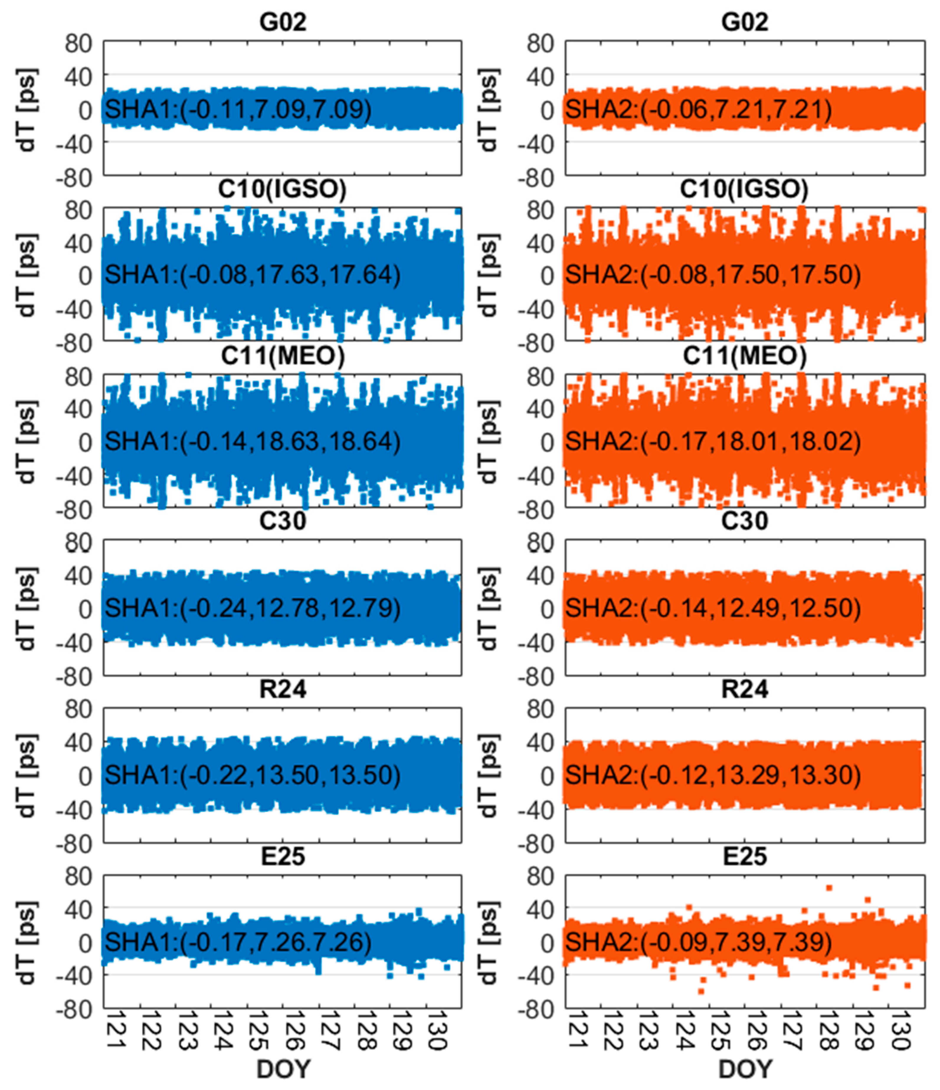
4.1. The ED Clock Offsets

The time series of estimated ED clock offsets and its comparison with GFZ rapid (GBM) and CODE final (COD) multi-GNSS products are depicted in Figure 5. To show ED clock offsets more clearly, the ED clock offsets are shifted by the same amount (1 ns) to avoid overlapping. Figure 6 shows their differences. Because BDS constellations are composed of Geostationary Earth Orbit (GEO), Inclined Geosynchronous Satellite Orbit (IGSO), and Medium Earth Orbit (MEO) satellites, different orbit types of BDS satellites have different accuracy in POD [28,29]. Therefore, the corresponding clock offsets have different accuracy for different orbit types. In order to analyze BDS-2 objectively, we discuss it separately. From Figure 5 and Figure 6, we can find that the difference between GBM and the estimated ED clock offsets for SHA1 and SHA2 is very small, and they are basically distributed on the diagonal with slope of 1. From Figure 5 and Figure 7, we can draw a similar conclusion that the estimated ED clock offsets are basically consistent with COD. This means that the performance of the estimated ED clock is basically consistent with GBM and COD. Certainly, we can also find that the performance of BDS-2 is slightly worse than other systems, especially for GEO satellites. There are three reasons for the difference. First, BDS-2 is a regional navigation system, and the stations tracked BDS-2 signals are basically located in Asia and Europe. There are less observations for BDS-2 POD and PCE because of the unevenly distributed stations. Secondly, BDS-2 contains five GEO and seven IGSO satellites. The orbit accuracy of BDS-2 GEO and IGSO satellites is poor due to the force models and the observation geometry. Therefore, the estimated ED clock offsets calculated by fixed GEO orbit is slightly poor. Last, but most important, there are some differences between GFZ and SHAO in BDS data processing strategies in terms of the precise attitude model, the solar radiation pressure model, and DCB corrections [11,30], which leads to the poor consistency of the results. In order to more accurately and objectively explain the accuracy of the estimated ED clock offsets compared with GBM and COD, the mean, STD, and RMS of the estimated ED clock offsets between GBM, COD and SHA1, SHA2 for multi-GNSS satellites are listed in

Table 2. The statistics of means, STD, and RMS for GPS, BDS-2 GEO, BDS-2 IGSO, BDS-2 MEO, BDS-3, GLONASS, and Galileo satellites ED clock (unit: ps).

	System	GPS	BDS-2 (GEO)	BDS-2 (IGSO)	BDS-2 (MEO)	BDS-3	GLONASS	Galileo
Type
SHA1 (GBM)	Mean	−0.26	0.96	−0.47	−0.30	−0.37	−0.20	−0.25
	STD	6.45	21.31	15.19	14.36	11.04	12.64	7.17
	RMS	6.46	21.33	15.20	14.36	11.05	12.65	7.17
SHA2 (GBM)	Mean	−0.13	0.94	−0.43	−0.25	−0.24	−0.13	−0.18
	STD	6.29	21.25	15.54	14.56	11.03	12.71	7.16
	RMS	6.32	21.27	15.55	14.57	11.03	12.71	7.16
SHA1 (COD)	Mean	−0.21	Non	−0.27	−0.22	−0.25	−0.11	−0.22
	STD	6.73	Non	14.93	14.50	11.22	12.61	6.87
	RMS	6.82	Non	15.01	14.52	11.24	12.71	6.90
SHA2 (COD)	Mean	−0.09	Non	−0.15	−0.17	−0.13	−0.03	−0.12
	STD	6.54	Non	15.46	13.90	11.46	13.26	7.32
	RMS	6.57	Non	15.50	14.00	11.48	13.30	7.34

. Our calculation is basically consistent with the results of GBM and COD. The difference in ED clock offsets between GBM, COD and SHA1, SHA2 for GPS and Galileo satellites range from 6 to 7 ps, and the difference for BDS and Galileo range from 10 to 16 ps. The results in Table 2 confirm the findings of Figure 5, Figure 6 and Figure 7.

Now, turn to the influence of tropospheric delays on ED clock offsets estimation. Figure 5, Figure 6 and Figure 7 not only show the difference between GBM, COD, and the estimated ED clock offsets but also depict the difference between SHA1 and SHA2. As shown in Figure 5, SHA1 and SHA2 are highly overlapped, and it is difficult to distinguish the difference. From Figure 6 and Figure 7 and Table 2, we can see that the difference between SHA1 and SHA2 is very small, ranging from 0 to 0.35 ps in terms of the statistics of mean, STD, and RMS for GPS, BDS-2 GEO, BDS-2 IGSO, BDS-2 MEO, BDS-3, GLONASS, and Galileo satellites, which can be ignored. To prove this point more favorably and reflect the situation of each satellite clearly, the relationship between SHA1 and SHA2 in terms of the mean, STD, and RMS of each satellite is depicted in Figure 8. The mean of each satellite for SHA2 is closer to 0 than SHA1, but the difference is very tiny. In addition, the STD and RMS of each satellite are basically distributed on the diagonal with slope of 1. In general, the ED clock of SHA1 and SHA2 are basically consistent both in mean, STD, and RMS. However, from a calculation time-consuming point of view, adding the ZWD parameter will increase the computation complexity. The corresponding time-consuming will increase. As shown in Figure 9, the mean time-consuming of SHA1 is about 16.5 min, and that of SHA2 is about 23.5 min, based on Lenovo SR650 server (4*Inter (R) Xeon (R) Gold 6244 CPU @3.60GHz) using OpenMP and Intel MKL. In case of poor data quality, the time-consuming of SHA1 is about 20 to 23 min. In normal conditions, SHA1 takes less than 20 min.

As mentioned above, the time-consuming of POD and high-rate PCE must be less than 1 h to achieve one-hourly updated orbits and clocks. Because the difference between SHA1 and SHA2 is very tiny, and its difference is less than 0.35 ps in terms of mean, STD, and RMS. As stated earlier, SHA1 can use the OpenMP for parallel processing of multiple stations, multiple epochs, and multiple satellites, while SHA2 can only use the OpenMP for parallel processing of multiple stations and multiple satellites. The computational efficiency of SHA1 is significantly higher than that of SHA2. Considering the calculation time and accuracy, SHA1 as the optimal strategy is applied to obtain one-hourly updated ultra-rapid clock.

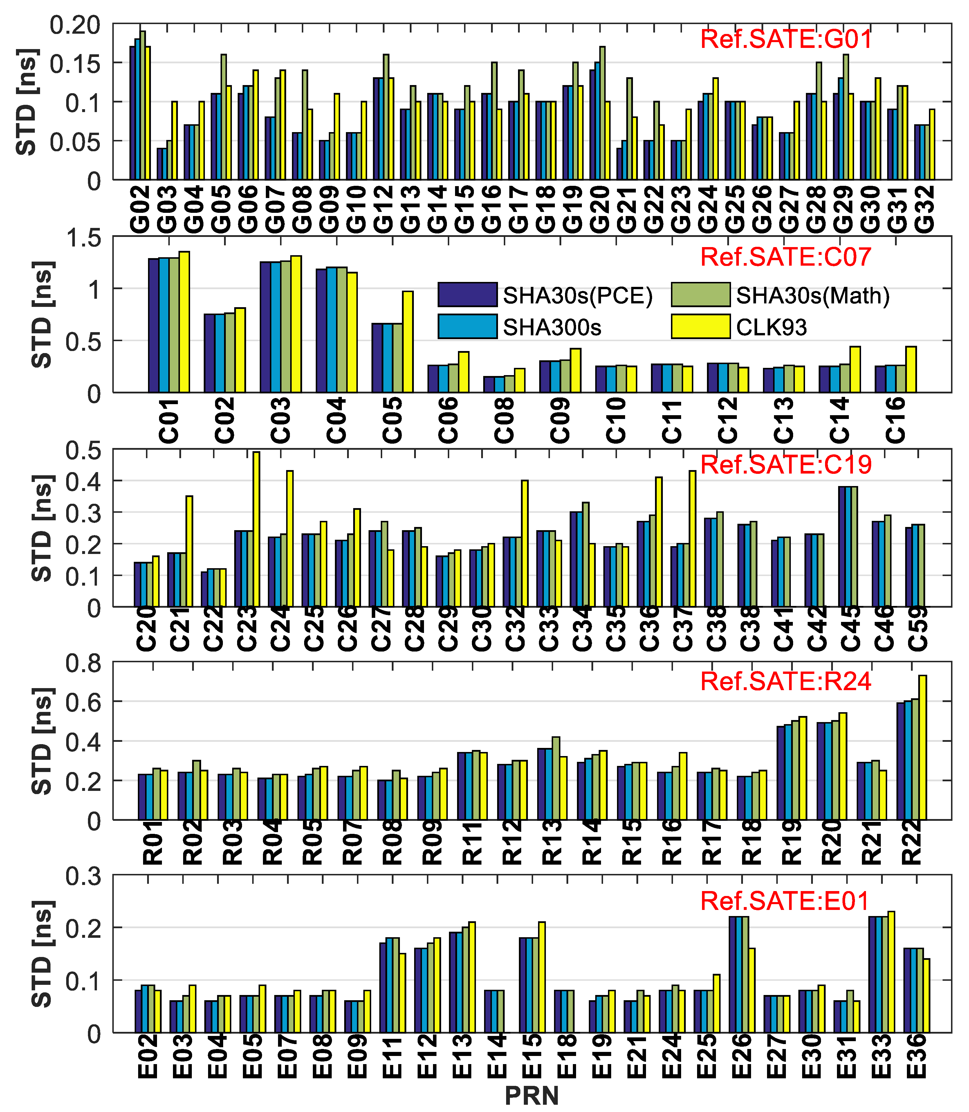
4.2. The Absolute Clock Offsets

The ED clock offsets calculated by the SHA1 strategy are restored to the absolute clock offsets by using Equation (6). The double-difference (DD) method of selecting one satellite to eliminate the clock datum [31] is used to assess the absolute clock. GPS PRN01 (G01), BDS-2 PRN07 (C07), BDS-3 PRN19 (C19), GLONASS PRN24 (R24), and Galileo PRN01 (E01) are selected as the reference satellite to assess the clock of other GNSS satellites. Figure 10 and Figure 11 show the STD and RMS of high-rate and low-rate one-hourly updated GNSS ultra-rapid clock for observation. In addition, the ultra-rapid products are more targeted to real-time and near real-time users; we added the real-time stream products CLK93 released by CNES to discuss the precision of estimated clock and CLK93. When users use the low-rate clock, they need to use mathematical interpolation algorithm to interpolate the low-rate clock, which causes the loss of clock accuracy [14]. In order to reflect the actual applications of low-rate clock, the clock interpolated by the ninth order Lagrange interpolation algorithm was also evaluated.

It can be seen from Figure 10 that the STD of the estimated high-rate clock (SHA30s (PCE)), low-rate clock (SHA300s), and clock offsets interpolated by mathematical interpolation algorithm (SHA30s (Math)) for GPS, BDS-2 GEO, BDS-2 non-GEO, BDS-3, GLONASS, and Galileo satellites are basically better than 0.2, 1.2, 0.3, 0.3, 0.4, and 0.2 ns, respectively. From SHA30s (PCE), SHA300s, and SHA30s (Math), we can find that SHA30s (PCE) has a certain improvement compared with SHA30s (Math), but the improvement is not obvious compared with SHA300s. There are three reasons for the little increase in SHA30s (PCE) compared with SHA300s. Firstly, the weight of the control points is higher than that of the ED clock offsets when the ED clock offsets are restored to the absolute clock offsets by using low-rate clock offsets as control points. Secondly, the accuracy of SHA300s is obtained by evaluating the clock offsets on time node (300s intervals), and there is no precision loss caused by the interpolation algorithm. Finally, the accuracy of SHA300s provide by SHAO is already good.

It is worth mentioning that the STD of the estimated clock offsets is slightly better than CLK93. There are two possible explanations: the clock offsets precision is inevitably disturbed by the stability of real-time observation streams, more commonly, the available observation data for real-time product solution are less than ultra-rapid solutions. In other words, one-hourly updated ultra-rapid orbit and clock offsets products can ensure better accuracy in the case of poor network environment. Whether it is used as backup data or practical data, one-hourly updated ultra-rapid orbit and clock offsets products are very reliable.

Note that RMS, the RMS of SHA30s (PCE), SHA300s, and SHA30s (Math) for GPS, BDS-2, BDS-3, GLONASS, and Galileo satellites are basically better than 0.5, 3.0, 0.9, 1.2, and 0.4 ns. The RMS of satellites such as G04, G14, G18, G23, C11, C12, and C14 are especially large compared with other satellites. Because the different ACs adopt different processing strategies such as the precise attitude model, the solar radiation pressure model, and DCB corrections [11,30,32], these inconsistencies lead to the differences between SHAO and GBM on some satellites. Moreover, the RMS of GLONASS satellites is worse than other GNSSs, which is due to the possible bias caused by the float ambiguity solutions in POD and frequency division multiple access (FDMA) signal transmit mechanism. From the comparison between SHA30s (PCE) and CLK93, we can find that the RMS of SHA30s (PCE) is better than that of CLK93. As commented earlier, the main reasons are as follows: on the one hand, different ACs have differences in data processing strategies, on the other hand, the available observation data for real-time product solution is not as stable as that of ultra-rapid solutions.

Now, pay attention to the mean STD and RMS for the observation session and prediction session. Combined with Figure 10, Figure 11 and Figure 12, we can obtain four key findings. In terms of the precision of the estimated high-rate clock offsets and SHAO low-rate clock offsets, GPS and Galileo are the best, BDS-3 is the second, and GLONASS and BDS-2 are relatively worse. Secondly, SHA30s (PCE) is optimal in both the observation and prediction session. The absolute clock of the prediction and observation sessions has been modified by the improvement of the time resolution. The STD and RMS are improved by (0.97 to 9.09% and 0.12 to 5.56%) in the observation session, (2.82 to 23.08% and 0.95 to 9.09%) in the first hour of the prediction session, and (0 to 3.85% and 0.12 to 4.19%) in the second hour of the prediction session, respectively. Thirdly, the precision of SHA30 (PCE) is slightly better than CLK93 in the observation section and basically the same as CLK93 in the prediction section. Finally, there are some differences between SHAO, GFZ, and CNES in the data processing strategy, and the clock offsets of different ACs show differences in RMS.

4.3. Real-Time PPP Validation

The RT-PPP experiments will be carried out to verify the practicability and reliability of the estimated clocks. The PPP solutions using GBM products (30 s interval) is taken as the reference. Figure 13 depicts the PPP convergence at HUEG for GPS-only, BDS-only, GLONASS-only, Galileo-only, and multi-GNSS (GPS + BDS + GLONASS + Galileo). To show the PPP convergence clearly, only the first 2 h are shown in Figure 13. From Figure 13, we can see that the convergence time for SHA30s (PCE) is obviously improved, and its performance is basically same as that of GBM products. Figure 14 shows the average convergence time. During the observation session, SHA30s (PCE) can improve the convergence time by (48.16, 31.55, 37.06%) for GPS-only PPP, (32.88, 21.96, 22.60%) for BDS-only PPP, (40.78, 31.15, 35.05%) for GLONASS-only PPP, (40.49, 23.49, 25.57%) for Galileo-only PPP, and (64.75, 60.28, 55.07%) for multi-GNSS PPP, compared with SHA300s in north, east, and up directions, respectively. In the first hour of the prediction session, SHA30s (PCE) can improve the convergence time by (49.84, 32.47, 37.63%) for GPS-only PPP, (33.62, 24.53, 28.12%) for BDS-only PPP, (44.16, 27.69, 28.69%) for GLONASS-only PPP, (44.82, 25.03, 23.95%) for Galileo-only PPP, and (65.75, 60.98, 56.21%) for multi-GNSS PPP, respectively. In the second hour of the prediction session, SHA30s (PCE) can improve the convergence time by (57.27, 34.85, 36.03%) for GPS-only PPP, (39.76, 27.80, 31.31%) for BDS-only PPP, (43.99, 28.29, 26.30%) for GLONASS-only PPP, (45.74, 26.30, 28.29%) for Galileo-only PPP, and (62.12, 55.51, 57.14%) for multi-GNSS PPP, respectively. The estimated high-rate one-hourly ultra-rapid clock greatly shortens the PPP convergence time, which is basically the same as GBM and slightly better than CLK93 in the observation session. In the prediction session, SHA30s (PCE) performs good, and the convergence time of SHA30s (PCE) is at the same level as CLK93.

As for positioning accuracy, the final convergence accuracy of SHA30s (PCE) and SHA300s is basically the same in the observation section. However, the positioning accuracy of SHA300s decreases slightly in the prediction session, while the performance of SHA30s (PCE) is still good. From the Figure 15 and Figure 16, it is obvious that the positioning accuracy will decrease with the increase in prediction time. However, using high-rate clock offsets can appropriately avoid the decrease in positioning accuracy. The positioning accuracy of SHA30s (PCE) for GPS-only, BDS-only, GLONASS-only, Galileo-only, and multi-GNSS PPP is improved by 14.90, 21.68, 13.38, 9.06, and 25.74% in the observation session, 12.34, 1.52, 13.37, 8.66, and 12.99% in the first hour of the prediction session, and 7.97, 9.86, 7.76, 22.45, and 11.65% in the second hour of the prediction session, respectively. Similarly, SHA30s (PCE) improves the PPP positioning accuracy, which is slightly better than CLK93 in the observation session. In the prediction session, the positioning accuracy of SHA30s (PCE) is at the same level as CLK93. Even in the case of poor network environment, the estimated high-rate one-hourly ultra-rapid clock can ensure the better PPP performance.

In summary, the estimated high-rate one-hourly ultra-rapid clock can improve the PPP performance in terms of positioning accuracy and convergence time and can be well applied to real-time PPP applications.

5. Conclusions

This contribution focused on the high-rate one-hourly updated ultra-rapid PCE and its application in RT-PPP. We modified the ED PCE model by investigating the influence of tropospheric delays on ED PCE and proposed a new framework to obtain high-rate one-hourly updated ultra-rapid clock. The OpenMP and Intel MKL are used to construct a parallel processing system to improve computation efficiency. Through the analysis and discussion, we can draw the following conclusions.

As for the influence of tropospheric delays on ED PCE, the difference between SHA1 and SHA2 is very tiny, ranging from 0 to 0.35 ps in terms of the statistics of mean, STD, and RMS for multi-GNSS satellites, which can be ignored. From a calculation time-consuming point of view, adding the ZWD parameter will increase the computation complexity. The corresponding time-consuming will increase. The time-consuming of SHA1 is about 16.5 min, and that of SHA2 is about 23.5 min based on the Lenovo SR650 server (4*Inter (R) Xeon (R) Gold 6244 CPU @3.60 GHz). Therefore, SHA1 as the optimal strategy with low time-consuming and high accuracy is recommended to obtain one-hourly updated ultra-rapid clock offsets. From the precision of the clock offsets point of view, improving the time resolution can improve the precision of the absolute clock offsets in both prediction and observation sessions. The STD and RMS are improved by (0.97 to 9.09% and 0.12 to 5.56%) in the observation session, (2.82 to 23.08% and 0.95 to 9.09%) in the first hour of the prediction session, and (0.11 to 3.85% and 0.12 to 4.19%) in the second hour of the prediction session, respectively.

Similarly, the estimated clock offsets perform well in RT-PPP. The estimated clock offsets improve the PPP positioning accuracy and greatly shorten the convergence time. The positioning accuracy can be improved by 9.06~25.74% in the observation session, 1.52~13.37% in the first hour of the prediction session, and 7.76~22.45% in the second hour of the prediction session, respectively. The convergence time can be significantly improved by 21.96~64.75, 23.95~65.75, and 26.30~62.12% for the observation session, the first hour of the prediction session, and the second hour of the prediction session compared with low-rate products, respectively. The RT-PPP performance of SHA30s (PCE) is basically the same as GFZ rapid products and slightly better than CLK93. Whether in the prediction session or in the observation session, the estimated clock shows good performance. The estimated high-rate one-hourly ultra-rapid clock can ensure the better PPP performance in the case of poor network environment.

Synthesizing the analysis and discussion above, the estimated high-rate one-hourly updated ultra-rapid precise clock offsets (URL: ftp://igsdepot.ign.fr/pub/igs/products/mgex/, accessed on 1 March 2022) have excellent performance, which can be well applied to real-time or near real-time applications and research.

References

1. Kouba, J. A Guide to Using International GNSS Service (IGS) Products; Jet Propulsion Laboratory: Pasadena, CA, USA, 2009; p. 34. Available online: http://igscb.jpl.nasa.gov/igscb/resource/pubs/GuidetoUsingIGSProducts.pdf (accessed on 1 March 2022).
2. Dow, J.M.; Neilan, R.E.; Rizos, C. The International GNSS Service in a changing landscape of Global Navigation Satellite Systems. J. Geod. 2009, 83, 191–198. [Google Scholar] [CrossRef]
3. Choi, K.K.; Ray, J.; Griffiths, J.; Bae, T.-S. Evaluation of GPS orbit prediction strategies for the IGS Ultra-rapid products. GPS Solut. 2012, 17, 403–412. [Google Scholar] [CrossRef]
4. Lutz, S.; Beutler, G.; Schaer, S.; Dach, R.; Jäggi, A. CODE’s new ultra-rapid orbit and ERP products for the IGS. GPS Solut. 2014, 20, 239–250. [Google Scholar] [CrossRef] [Green Version]
5. Elsobeiey, M.; Al-Harbi, S. Performance of real-time Precise Point Positioning using IGS real-time service. GPS Solut. 2015, 20, 565–571. [Google Scholar] [CrossRef]
6. Laurichesse, D.; Cerri, L.; Berthias, J.P.; Mercier, F. Real Time Precise GPS Constellation and Clocks Estimation by Means of a Kalman Filter. In Proceedings of the 26th International Technical Meeting of the Satellite Division of The Institute of Navigation (ION GNSS + 2013), Nashville, TN, USA, 16–20 September 2013; pp. 1155–1163. [Google Scholar]
7. Ge, M.; Chen, J.; Douša, J.; Gendt, G.; Wickert, J. A computationally efficient approach for estimating high-rate satellite clock corrections in realtime. GPS Solut. 2011, 16, 9–17. [Google Scholar] [CrossRef]
8. Ge, M.; Gendt, G.; Dick, G.; Zhang, F.P.; Rothacher, M. A New Data Processing Strategy for Huge GNSS Global Networks. J. Geod. 2006, 80, 199–203. [Google Scholar] [CrossRef]
9. Zuo, X.; Jiang, X.; Li, P.; Wang, J.; Ge, M.; Schuh, H. A square root information filter for multi-GNSS real-time precise clock estimation. Satell. Navig. 2021, 2, 28. [Google Scholar] [CrossRef]
10. Li, X.; Chen, X.; Ge, M.; Schuh, H. Improving multi-GNSS ultra-rapid orbit determination for real-time precise point positioning. J. Geod. 2018, 93, 45–64. [Google Scholar] [CrossRef]
11. Chen, Q.; Song, S.; Zhou, W. Accuracy Analysis of GNSS Hourly Ultra-Rapid Orbit and Clock Products from SHAO AC of iGMAS. Remote Sens. 2021, 13, 1022. [Google Scholar] [CrossRef]
12. Guo, J.; Xu, X.; Zhao, Q.; Liu, J. Precise orbit determination for quad-constellation satellites at Wuhan University: Strategy, result validation, and comparison. J. Geod. 2015, 90, 143–159. [Google Scholar] [CrossRef]
13. Ma, H.; Zhao, Q.; Xu, X. A New Method and Strategy for Precise Ultra-Rapid Orbit Determination. In Proceedings of the China Satellite Navigation Conference (CSNC), Shanghai, China, 23–25 May 2017; Lecture Notes in Electrical Engineering. Springer: Singapore, 2017; pp. 191–205. [Google Scholar]
14. Guo, F.; Zhang, X.; Li, X.; Cai, S. Impact of sampling rate of IGS satellite clock on precise point positioning. Geo-Spat. Inf. Sci. 2010, 13, 150–156. [Google Scholar] [CrossRef]
15. Zhang, X.; Li, X.; Guo, F. Satellite clock estimation at 1 Hz for realtime kinematic PPP applications. GPS Solut. 2010, 15, 315–324. [Google Scholar] [CrossRef]
16. Hein, G.W. Status, perspectives and trends of satellite navigation. Satell. Navig. 2020, 1, 22. [Google Scholar] [CrossRef] [PubMed]
17. Bahadur, B.; Nohutcu, M. Comparative analysis of MGEX products for post-processing multi-GNSS PPP. Measurement 2019, 145, 361–369. [Google Scholar] [CrossRef]
18. Bock, H.; Dach, R.; Jäggi, A.; Beutler, G. High-rate GPS clock corrections from CODE: Support of 1 Hz applications. J. Geod. 2009, 83, 1083–1094. [Google Scholar] [CrossRef] [Green Version]
19. Ye, S.; Zhao, L.; Song, J.; Chen, D.; Jiang, W. Analysis of estimated satellite clock biases and their effects on precise point positioning. GPS Solut. 2017, 22, 16. [Google Scholar] [CrossRef]
20. Zhang, W.; Lou, Y.; Gu, S.; Shi, C.; Haase, J.S.; Liu, J. Joint estimation of GPS/BDS real-time clocks and initial results. GPS Solut. 2015, 20, 665–676. [Google Scholar] [CrossRef]
21. Zhang, Q.; Moore, P.; Hanley, J.; Martin, S. Auto-BAHN: Software for near real-time GPS orbit and clock computations. Adv. Space Res. 2007, 39, 1531–1538. [Google Scholar] [CrossRef]
22. Landskron, D.; Bohm, J. VMF3/GPT3: Refined discrete and empirical troposphere mapping functions. J. Geod. 2018, 92, 349–360. [Google Scholar] [CrossRef]
23. Montenbruck, O.; Steigenberger, P.; Prange, L.; Deng, Z.; Zhao, Q.; Perosanz, F.; Romero, I.; Noll, C.; Stürze, A.; Weber, G.; et al. The Multi-GNSS Experiment (MGEX) of the International GNSS Service (IGS)–Achievements, prospects and challenges. Adv. Space Res. 2017, 59, 1671–1697. [Google Scholar] [CrossRef]
24. Rebischung, P.; Schmid, R. IGS14/igs14.atx: A new framework for the IGS products. In Proceedings of the AGU Fall Meeting 2016, San Francisco, CA, USA, 12–16 December 2016; Volume 121, pp. 6109–6131. [Google Scholar]
25. Wu, J.-T.; Wu, S.C.; Hajj, G.A.; Bertiger, W.I.; Lichten, S.M. Effects of antenna orientation on GPS carrier phase. In Proceedings of the Astrodynamics 1991, San Diego, CA, USA, 19–22 August 1991; pp. 1647–1660. [Google Scholar]
26. Petit, G.; Luzum, B. IERS Conventions(2010); IERS Technical Note No. 36; Verlag des Bundesamts für Kartographie und Geodäsie: Frankfurt am Main, Germany, 2010. [Google Scholar]
27. Zhou, W.; Huang, C.; Song, S.; Chen, Q.; Liu, Z. Characteristic Analysis and Short-Term Prediction of GPS/BDS Satellite Clock Correction. In Proceedings of the China Satellite Navigation Conference (CSNC) 2016 Proceedings: Volume III, Changsha, China, 27 April 2016; pp. 187–200. [Google Scholar] [CrossRef]
28. Yang, Y.; Gao, W.; Guo, S.; Mao, Y.; Yang, Y. Introduction to BeiDou-3 navigation satellite system. Navigation 2019, 66, 7–18. [Google Scholar] [CrossRef] [Green Version]
29. Yang, Y.; Li, J.; Wang, A.; Xu, J.; He, H.; Guo, H.; Shen, J.; Dai, X. Preliminary assessment of the navigation and positioning performance of BeiDou regional navigation satellite system. Sci. China Earth Sci. 2013, 57, 144–152. [Google Scholar] [CrossRef]
30. Deng, Z.; Ge, M.; Uhlemann, M.; Zhao, Q. Precise orbit determination of BeiDou satellites at GFZ. In Proceedings of the IGS Workshop, Vienna, Austria, 2 May 2014; pp. 23–27. [Google Scholar]
31. Yao, Y.; He, Y.; Yi, W.; Song, W.; Cao, C.; Chen, M. Method for evaluating real-time GNSS satellite clock offset products. GPS Solut. 2017, 21, 1417–1425. [Google Scholar] [CrossRef]
32. Uhlemann, M.; Gendt, G.; Ramatschi, M.; Deng, Z. GFZ global multi-GNSS network and data processing results. In IAG 150 Years; Springer: Berlin/Heidelberg, Germany, 2015; pp. 673–679. [Google Scholar]
Figure 1. The number of estimated parameters for the different PCE models with the increase in the number of the tracking stations, in which UD PCE, ED PCE, and MED PCE denote undifferenced ionosphere-free PCE model, epoch-difference PCE model, and modified epoch-difference PCE, respectively. Suppose a station can track six satellites for each constellation in one epoch.
Remotesensing 14 01257 g001
Figure 2. Distribution of the selected GNSS tracking stations for PCE and PPP, in which the stations marked red are used for PCE and the stations marked blue are used for RT-PPP.
Remotesensing 14 01257 g002
Figure 3. The slide window for one-hourly updated ultra-rapid orbit and clock offsets products generation.
Remotesensing 14 01257 g003
Figure 4. The data processing flow for one-hourly updated ultra-rapid orbit and clock offsets products generation.
Remotesensing 14 01257 g004
Figure 5. The time series of estimated ED clock offsets and its comparison with GFZ rapid and COD final clock products, in which CC denotes the correlation coefficient.
Remotesensing 14 01257 g005
Figure 6. The difference between GFZ rapid clock offsets and estimated ED clock offsets, in which (a, b, c) denotes (mean, STD, and RMS).
Remotesensing 14 01257 g006
Figure 7. The difference between CODE final clock offsets and estimated ED clock offsets, in which (a, b, c) denotes (mean, STD, and RMS).
Remotesensing 14 01257 g007
Figure 8. The mean, STD, and RMS of each satellite for GPS, BDS-2, BDS-3, GLONASS, and Galileo using two tropospheric processing strategies.
Remotesensing 14 01257 g008
Figure 9. The computation time for 1-day high-rate multi-GNSS PCE using 120 GNSS tracking stations, in which Non, OMP, and MKL denote no acceleration method, OpenMP, and Intel MKL, respectively.
Remotesensing 14 01257 g009
Figure 10. The STD of multi-GNSS ultra-rapid estimated clock for observation session, in which SHA30s (PCE), SHA300s, SHA30s (Math), and CLK93 depict the estimated high-rate clock, low-rate clock, clock interpolated by mathematical interpolation algorithm, and CNES real-time clock, respectively. The Ref.SATE means the reference satellite.
Remotesensing 14 01257 g010
Figure 11. The RMS of high-rate and low-rate one-hourly updated GNSS ultra-rapid clock for observation session, in which SHA30s (PCE), SHA300s, SHA30s (Math), and CLK93 depict the estimated high-rate clock, low-rate clock, clock interpolated by mathematical interpolation algorithm, and CNES real-time clock, respectively.
Remotesensing 14 01257 g011
Figure 12. Average STD and RMS of high-rate and low-rate one-hourly updated GNSS ultra-rapid clock for observation session and prediction session.
Remotesensing 14 01257 g012
Figure 13. PPP convergence at HUEG for GPS-only, BDS-only, GLONASS-only, Galileo-only, and multi-GNSS (GPS + BDS + GLONASS + Galileo) from 0:00 to 2:00 on DOY 121, 2021.
Remotesensing 14 01257 g013
Figure 14. The average convergence time for GPS-only, BDS-only, GLONASS-only, Galileo-only, and multi-GNSS PPP from DOY 121 to 130, 2021.
Remotesensing 14 01257 g014
Figure 15. PPP positioning error at HUEG for GPS-only, BDS-only, GLONASS-only, Galileo-only, and multi-GNSS from 20:00 on DOY 121 to 2:00 on DOY 122, 2021.
Remotesensing 14 01257 g015
Figure 16. The average RMS for GPS-only, BDS-only, GLONASS-only, Galileo-only, and multi-GNSS PPP from DOY 121 to 130, 2021.
Remotesensing 14 01257 g016