
Urban Flood Detection Using TerraSAR-X and SAR Simulated Reflectivity Maps


Abstract
:
1. Introduction
1.1. General
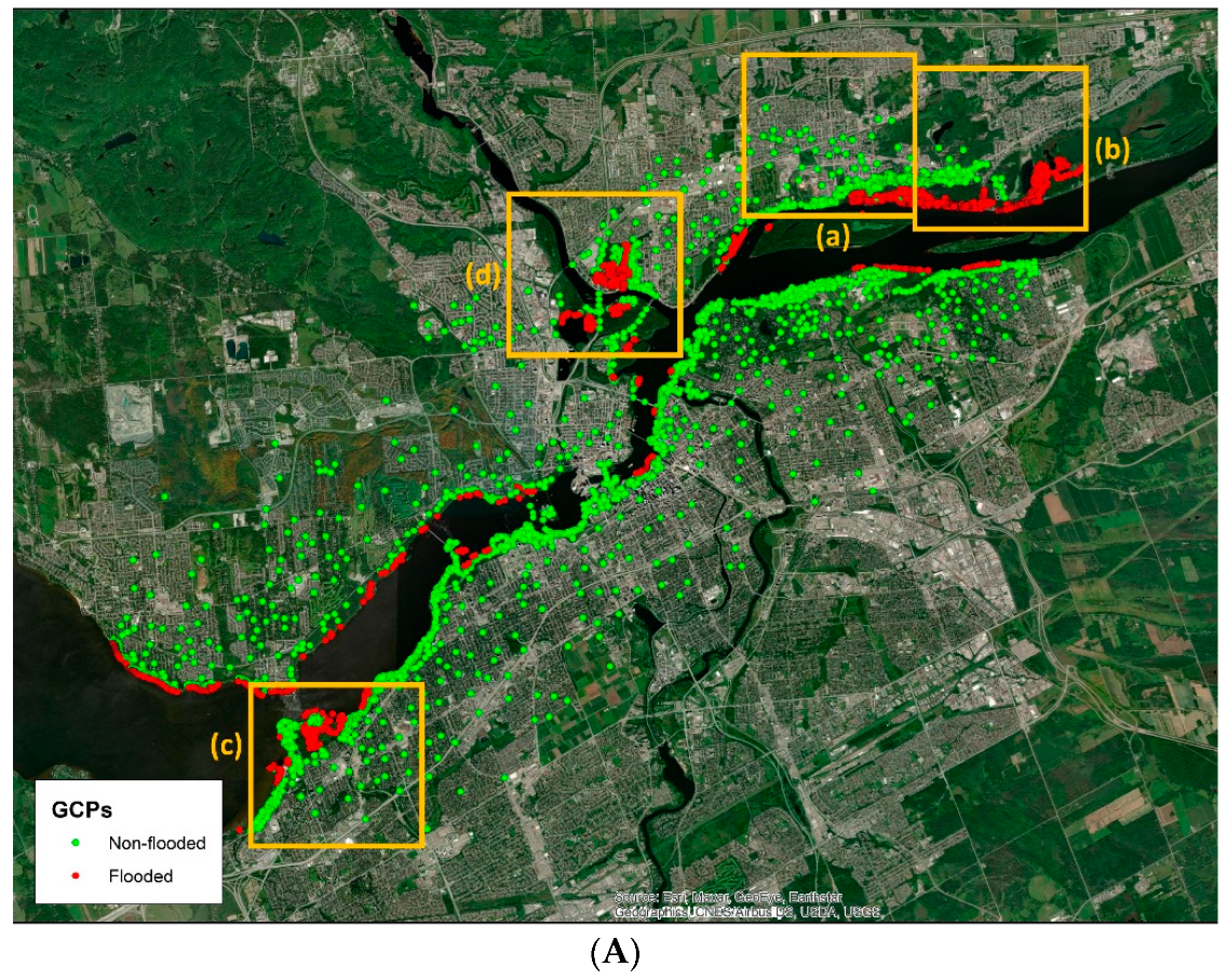
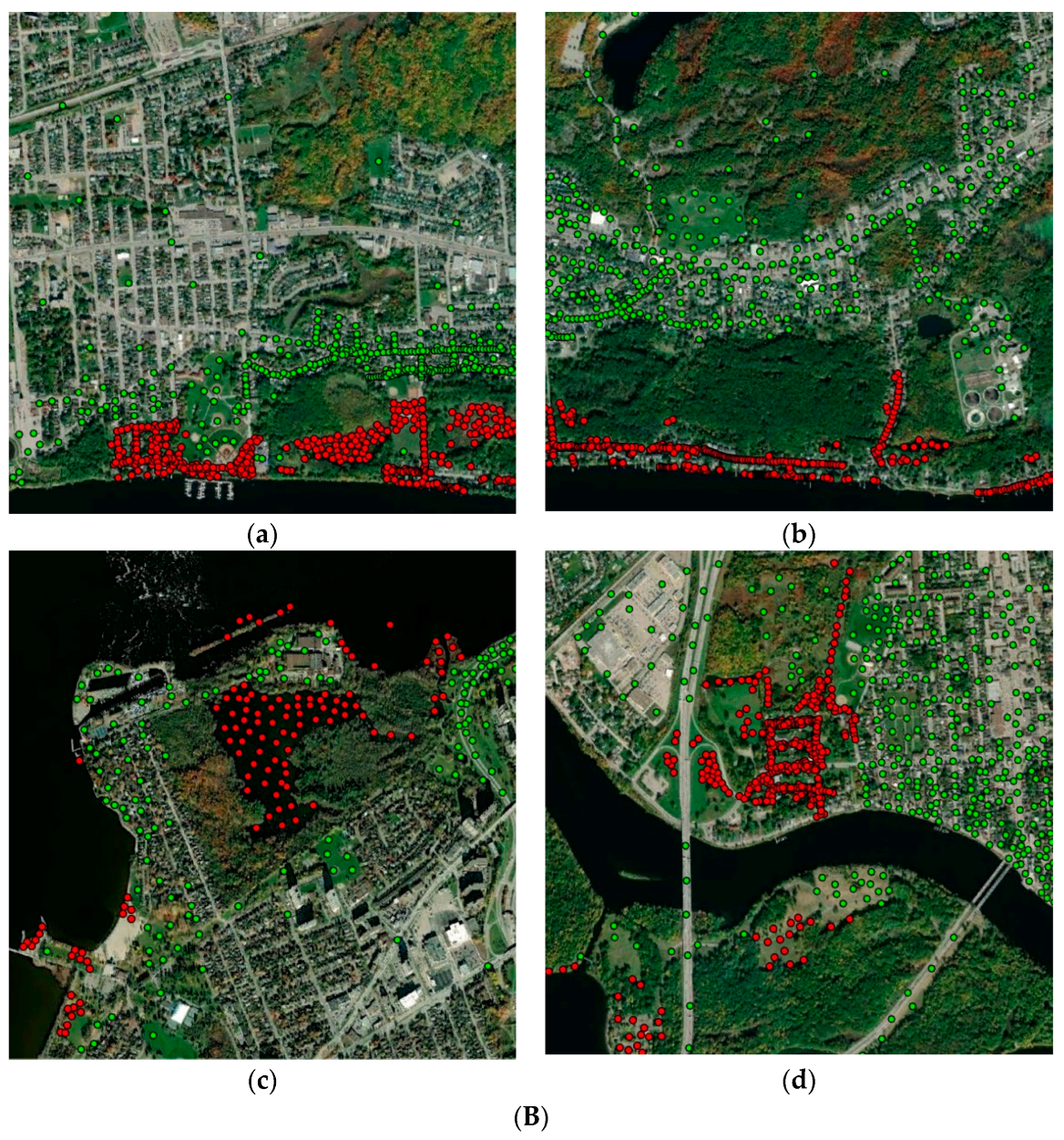
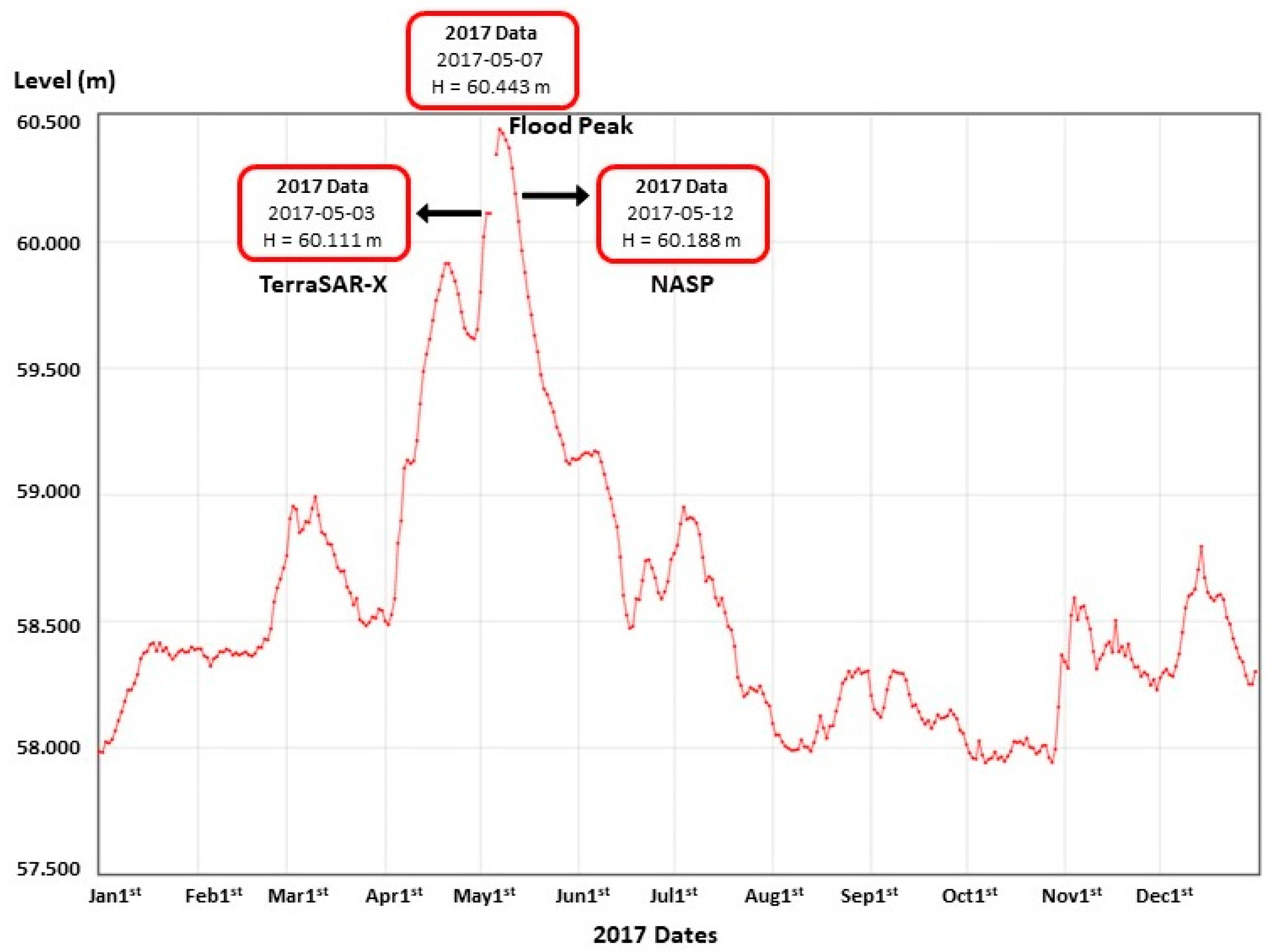
1.2. Study Area
1.3. Datasets
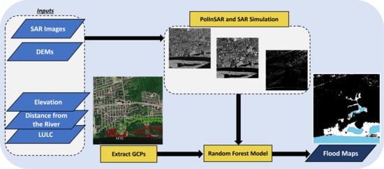
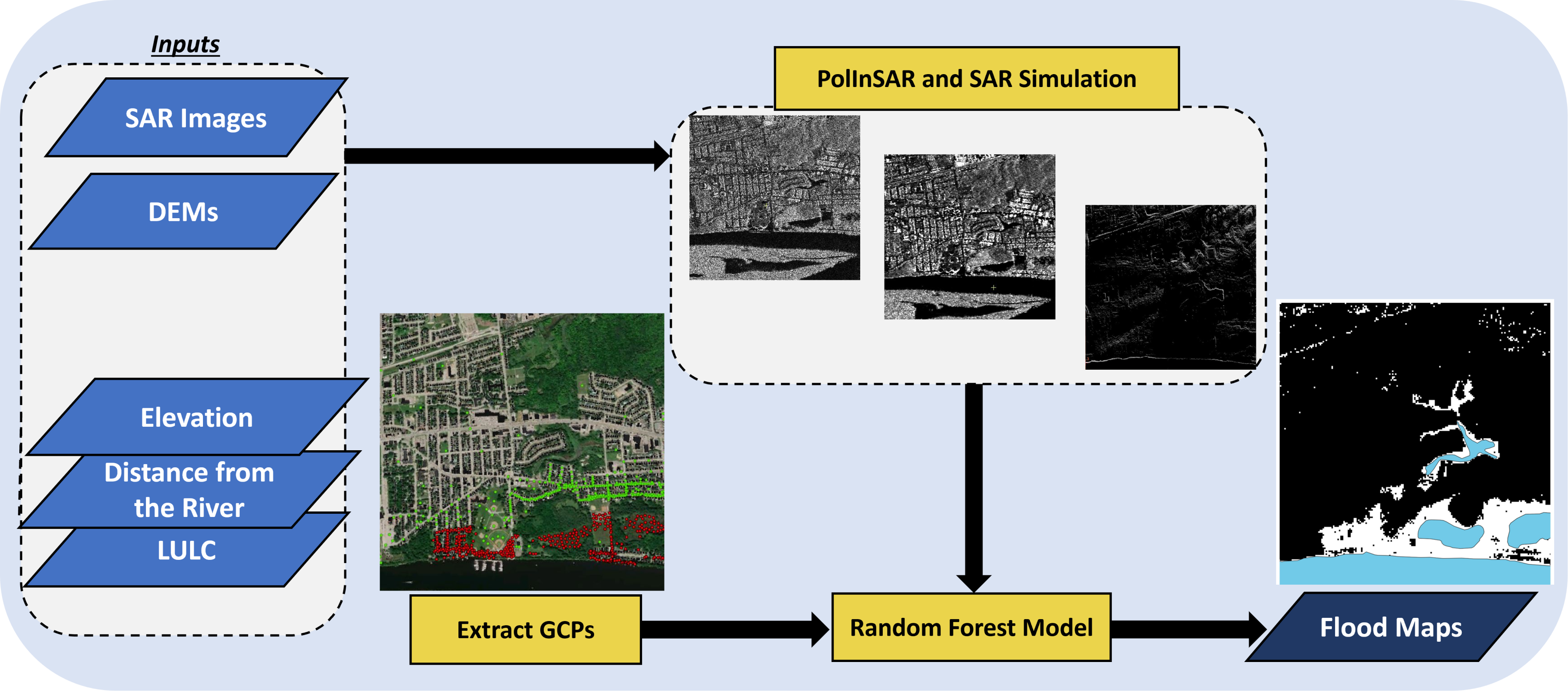
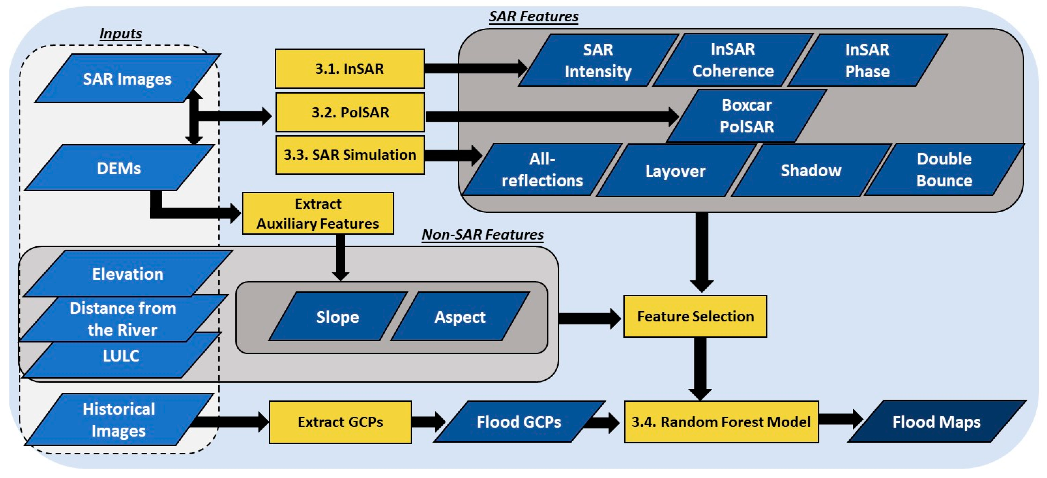
2. Methodology
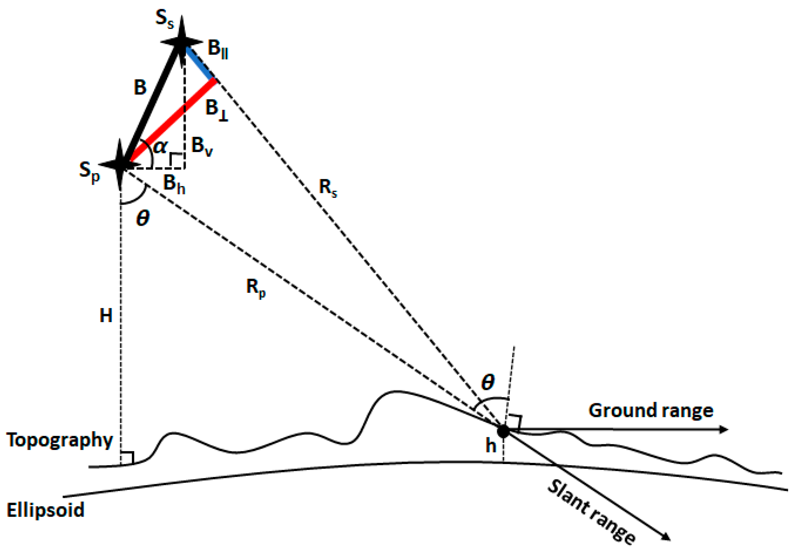
2.1. Interferometric SAR
2.2. Polarimetric SAR
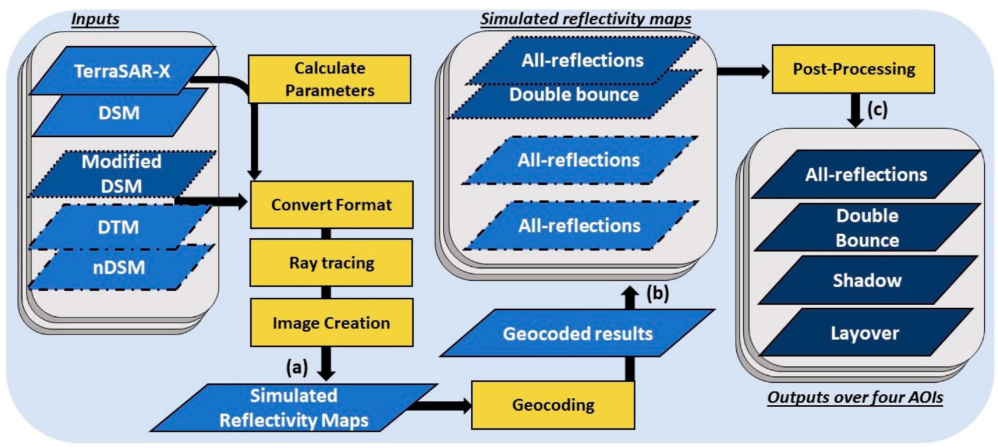
2.3. SAR Simulation
2.4. Random Forest Model
3. Results
4. Discussion
5. Conclusions
Author Contributions
Funding
Acknowledgments
Conflicts of Interest
References
- Olthof, I.; Svacina, N. Testing Urban Flood Mapping Approaches from Satellite and In-Situ Data Collected during 2017 and 2019 Events in Eastern Canada. Remote Sens. 2020, 12, 3141. [Google Scholar] [CrossRef]
- Willner, S.N.; Otto, C.; Levermann, A. Global Economic Response to River Floods. Nat. Clim. Chang. 2018, 8, 594–598. [Google Scholar] [CrossRef]
- Kundzewicz, Z.W.; Kanae, S.; Seneviratne, S.I.; Handmer, J.; Nicholls, N.; Peduzzi, P.; Mechler, R.; Bouwer, L.M.; Arnell, N.; Mach, K. Flood Risk and Climate Change: Global and Regional Perspectives. Hydrol. Sci. J. 2014, 59, 1–28. [Google Scholar] [CrossRef] [Green Version]
- Hirabayashi, Y.; Mahendran, R.; Koirala, S.; Konoshima, L.; Yamazaki, D.; Watanabe, S.; Kim, H.; Kanae, S. Global Flood Risk under Climate Change. Nat. Clim. Chang. 2013, 3, 816–821. [Google Scholar] [CrossRef]
- Lin, Y.N.; Yun, S.-H.; Bhardwaj, A.; Hill, E.M. Urban Flood Detection with Sentinel-1 Multi-Temporal Synthetic Aperture Radar (SAR) Observations in a Bayesian Framework: A Case Study for Hurricane Matthew. Remote Sens. 2019, 11, 1778. [Google Scholar] [CrossRef]
- Chini, M.; Pelich, R.; Pulvirenti, L.; Pierdicca, N.; Hostache, R.; Matgen, P. Sentinel-1 InSAR Coherence to Detect Floodwater in Urban Areas: Houston and Hurricane Harvey as a Test Case. Remote Sens. 2019, 11, 107. [Google Scholar] [CrossRef] [Green Version]
- Li, Y.; Martinis, S.; Wieland, M. Urban Flood Mapping with an Active Self-Learning Convolutional Neural Network Based on TerraSAR-X Intensity and Interferometric Coherence. ISPRS J. Photogramm. Remote Sens. 2019, 152, 178–191. [Google Scholar] [CrossRef]
- Amitrano, D.; Di Martino, G.; Iodice, A.; Riccio, D.; Ruello, G. Unsupervised Rapid Flood Mapping Using Sentinel-1 GRD SAR Images. IEEE Trans. Geosci. Remote Sens. 2018, 56, 3290–3299. [Google Scholar] [CrossRef]
- Wang, Y. Using Landsat 7 TM Data Acquired Days after a Flood Event to Delineate the Maximum Flood Extent on a Coastal Floodplain. Int. J. Remote Sens. 2004, 25, 959–974. [Google Scholar] [CrossRef]
- Reinartz, P.; Müller, R.; Suri, S.; Schwind, P.; Schneider, M. Terrasar-x Data for Improving Geometric Accuracy of Optical High and Very High Resolution Satellite Data. Available online: https://www.isprs.org/proceedings/XXXVIII/part1/11/11_01_Paper_17.pdf (accessed on 8 November 2022).
- Giustarini, L.; Hostache, R.; Matgen, P.; Schumann, G.J.-P.; Bates, P.D.; Mason, D.C. A Change Detection Approach to Flood Mapping in Urban Areas Using TerraSAR-X. IEEE Trans. Geosci. Remote Sens. 2012, 51, 2417–2430. [Google Scholar] [CrossRef]
- Mason, D.C.; Speck, R.; Devereux, B.; Schumann, G.J.-P.; Neal, J.C.; Bates, P.D. Flood Detection in Urban Areas Using TerraSAR-X. IEEE Trans. Geosci. Remote Sens. 2009, 48, 882–894. [Google Scholar] [CrossRef] [Green Version]
- Refice, A.; Capolongo, D.; Pasquariello, G.; D’Addabbo, A.; Bovenga, F.; Nutricato, R.; Lovergine, F.P.; Pietranera, L. SAR and InSAR for Flood Monitoring: Examples with COSMO-SkyMed Data. IEEE J. Sel. Top. Appl. Earth Obs. Remote Sens. 2014, 7, 2711–2722. [Google Scholar] [CrossRef]
- Uddin, K.; Matin, M.A.; Meyer, F.J. Operational Flood Mapping Using Multi-Temporal Sentinel-1 SAR Images: A Case Study from Bangladesh. Remote Sens. 2019, 11, 1581. [Google Scholar] [CrossRef] [Green Version]
- Martinis, S.; Twele, A.; Voigt, S. Towards Operational near Real-Time Flood Detection Using a Split-Based Automatic Thresholding Procedure on High Resolution TerraSAR-X Data. Nat. Hazards Earth Syst. Sci. 2009, 9, 303–314. [Google Scholar] [CrossRef]
- Pulvirenti, L.; Chini, M.; Pierdicca, N.; Guerriero, L.; Ferrazzoli, P. Flood Monitoring Using Multi-Temporal COSMO-SkyMed Data: Image Segmentation and Signature Interpretation. Remote Sens. Environ. 2011, 115, 990–1002. [Google Scholar] [CrossRef]
- Tanguy, M.; Chokmani, K.; Bernier, M.; Poulin, J.; Raymond, S. River Flood Mapping in Urban Areas Combining Radarsat-2 Data and Flood Return Period Data. Remote Sens. Environ. 2017, 198, 442–459. [Google Scholar] [CrossRef] [Green Version]
- Kwak, Y.; Yun, S.; Iwami, Y. A New Approach for Rapid Urban Flood Mapping Using ALOS-2/PALSAR-2 in 2015 Kinu River Flood, Japan. In Proceedings of the 2017 IEEE International Geoscience and Remote Sensing Symposium (IGARSS), Fort Worth, TX, USA, 23–28 July 2017; IEEE: Piscataway, NJ, USA, 2017; pp. 1880–1883. [Google Scholar]
- Mason, D.C.; Davenport, I.J.; Neal, J.C.; Schumann, G.J.-P.; Bates, P.D. Near Real-Time Flood Detection in Urban and Rural Areas Using High-Resolution Synthetic Aperture Radar Images. IEEE Trans. Geosci. Remote Sens. 2012, 50, 3041–3052. [Google Scholar] [CrossRef] [Green Version]
- Hess, L.L.; Melack, J.M.; Simonett, D.S. Radar Detection of Flooding beneath the Forest Canopy: A Review. Int. J. Remote Sens. 1990, 11, 1313–1325. [Google Scholar] [CrossRef]
- Horritt, M.S.; Mason, D.C.; Luckman, A.J. Flood Boundary Delineation from Synthetic Aperture Radar Imagery Using a Statistical Active Contour Model. Int. J. Remote Sens. 2001, 22, 2489–2507. [Google Scholar] [CrossRef]
- Shen, X.; Wang, D.; Mao, K.; Anagnostou, E.; Hong, Y. Inundation Extent Mapping by Synthetic Aperture Radar: A Review. Remote Sens. 2019, 11, 879. [Google Scholar] [CrossRef]
- Matgen, P.; Hostache, R.; Schumann, G.; Pfister, L.; Hoffmann, L.; Savenije, H.H.G. Towards an Automated SAR-Based Flood Monitoring System: Lessons Learned from Two Case Studies. Phys. Chem. Earth Parts A/B/C 2011, 36, 241–252. [Google Scholar] [CrossRef]
- Ohki, M.; Tadono, T.; Itoh, T.; Ishii, K.; Yamanokuchi, T.; Watanabe, M.; Shimada, M. Flood Area Detection Using PALSAR-2 Amplitude and Coherence Data: The Case of the 2015 Heavy Rainfall in Japan. IEEE J. Sel. Top. Appl. Earth Obs. Remote Sens. 2019, 12, 2288–2298. [Google Scholar] [CrossRef]
- Chaabani, C.; Chini, M.; Abdelfattah, R.; Hostache, R.; Chokmani, K. Flood Mapping in a Complex Environment Using Bistatic TanDEM-X/TerraSAR-X InSAR Coherence. Remote Sens. 2018, 10, 1873. [Google Scholar] [CrossRef] [Green Version]
- Pelich, R.; Chini, M.; Hostache, R.; Matgen, P.; Pulvirenti, L.; Pierdicca, N. Mapping Floods in Urban Areas from Dual-Polarization InSAR Coherence Data. IEEE Geosci. Remote Sens. Lett. 2021, 19, 4018405. [Google Scholar] [CrossRef]
- Zhao, J.; Li, Y.; Matgen, P.; Pelich, R.; Hostache, R.; Wagner, W.; Chini, M. Urban-Aware U-Net for Large-Scale Urban Flood Mapping Using Multitemporal Sentinel-1 Intensity and Interferometric Coherence. IEEE Trans. Geosci. Remote Sens. 2022, 60, 4209121. [Google Scholar] [CrossRef]
- Baghermanesh, S.S.; Jabari, S.; McGrath, H. Urban Flood Detection Using Sentinel1-A Images. In Proceedings of the 2021 IEEE International Geoscience and Remote Sensing Symposium IGARSS, Brussels, Belgium, 11–16 July 2021; IEEE: Piscataway, NJ, USA, 2021; pp. 527–530. [Google Scholar]
- Ferretti, A.; Monti-Guarnieri, A.; Prati, C.; Rocca, F. InSAR Principles: Guidelines for SAR Interferometry Processing and Interpretation; ESA: Paris, France, 2007.
- Ustuner, M.; Balik Sanli, F. Polarimetric Target Decompositions and Light Gradient Boosting Machine for Crop Classification: A Comparative Evaluation. ISPRS Int. J. Geo-Inf. 2019, 8, 97. [Google Scholar] [CrossRef] [Green Version]
- Han, Y.; Shao, Y. Full Polarimetric SAR Classification Based on Yamaguchi Decomposition Model and Scattering Parameters. In Proceedings of the 2010 IEEE International Conference on Progress in Informatics and Computing, Shanghai, China, 10–12 December 2010; IEEE: Piscataway, NJ, USA, 2010; Volume 2, pp. 1104–1108. [Google Scholar]
- Charbonneau, F.J.; Brisco, B.; Raney, R.K.; McNairn, H.; Liu, C.; Vachon, P.W.; Shang, J.; DeAbreu, R.; Champagne, C.; Merzouki, A. Compact Polarimetry Overview and Applications Assessment. Can. J. Remote Sens. 2010, 36, S298–S315. [Google Scholar] [CrossRef]
- Mohammadimanesh, F.; Salehi, B.; Mahdianpari, M.; Brisco, B.; Gill, E. Full and Simulated Compact Polarimetry Sar Responses to Canadian Wetlands: Separability Analysis and Classification. Remote Sens. 2019, 11, 516. [Google Scholar] [CrossRef] [Green Version]
- Tao, J.; Auer, S.; Palubinskas, G.; Reinartz, P.; Bamler, R. Automatic SAR Simulation Technique for Object Identification in Complex Urban Scenarios. IEEE J. Sel. Top. Appl. Earth Obs. Remote Sens. 2013, 7, 994–1003. [Google Scholar] [CrossRef]
- Mason, D.C.; Giustarini, L.; Garcia-Pintado, J.; Cloke, H.L. Detection of Flooded Urban Areas in High Resolution Synthetic Aperture Radar Images Using Double Scattering. Int. J. Appl. Earth Obs. Geoinf. 2014, 28, 150–159. [Google Scholar] [CrossRef]
- Esfandiari, M.; Jabari, S.; McGrath, H.; Coleman, D. Flood mapping using random forest and identifying the essential conditioning factors; a case study in fredericton, new brunswick, canada. ISPRS Ann. Photogramm. Remote Sens. Spat. Inf. Sci. 2020, 5, 609–615. [Google Scholar] [CrossRef]
- Kia, M.B.; Pirasteh, S.; Pradhan, B.; Mahmud, A.R.; Sulaiman, W.N.A.; Moradi, A. An Artificial Neural Network Model for Flood Simulation Using GIS: Johor River Basin, Malaysia. Environ. Earth Sci. 2012, 67, 251–264. [Google Scholar] [CrossRef]
- Ottawa River Regulation Planning Board. Summary of the 2017 Spring Flood; Ottawa River Regulation Planning Board: Ottawa, ON, Cannad, 2018.
- Hooper, A.J. Persistent Scatter Radar Interferometry for Crustal Deformation Studies and Modeling of Volcanic Deformation; Stanford University: Stanford, CA, USA, 2006. [Google Scholar]
- Yu, H.; Lan, Y.; Yuan, Z.; Xu, J.; Lee, H. Phase Unwrapping in InSAR: A Review. IEEE Geosci. Remote Sens. Mag. 2019, 7, 40–58. [Google Scholar] [CrossRef]
- Ferretti, A.; Prati, C.; Rocca, F. Multibaseline Phase Unwrapping for InSAR Topography Estimation. Nuovo Cim. C 2001, 24, 159–176. [Google Scholar]
- Bouchemakh, L.; Smara, Y.; Boutarfa, S.; Hamadache, Z. A Comparative Study of Speckle Filtering in Polarimetric Radar SAR Images. In Proceedings of the 2008 3rd International Conference on Information and Communication Technologies: From Theory to Applications, Damascus, Syria, 7–11 April 2008; IEEE: Piscataway, NJ, USA, 2008; pp. 1–6. [Google Scholar]
- Auer, S.J. 3D Synthetic Aperture Radar Simulation forInterpreting Complex Urban Re Scenarios. Doctoral Dissertation, Technische Universität München, Munich, Germany, 2011. [Google Scholar]
- Auer, S.; Hinz, S.; Bamler, R. Ray-Tracing Simulation Techniques for Understanding High-Resolution SAR Images. IEEE Trans. Geosci. Remote Sens. 2009, 48, 1445–1456. [Google Scholar] [CrossRef] [Green Version]
- Whitted, T. An Improved Illumination Model for Shaded Display. ACM Siggraph 2005 Courses 2005, 4-es. Available online: https://dl.acm.org/doi/abs/10.1145/1198555.1198743?casa_token=ZbzPioz44b0AAAAA:zzFPIwPE7A6sxS2AzuxUfGNyV9l6H7x7XcDKqkTSQivavwXtxsA63_HC8H8EAIGBPfO9hbUrS5BeYMQ (accessed on 8 November 2022).
- Glassner, A.S. An Introduction to Ray Tracing; Morgan Kaufmann: Burlington, MA, USA, 1989. [Google Scholar]
- Breiman, L. Random Forests. Mach. Learn. 2001, 45, 5–32. [Google Scholar] [CrossRef] [Green Version]
- Huo, J.; Shi, T.; Chang, J. Comparison of Random Forest and SVM for Electrical Short-Term Load Forecast with Different Data Sources. In Proceedings of the 2016 7th IEEE International conference on software engineering and service science (ICSESS), Beijing, China, 26–28 August 2016; IEEE: Piscataway, NJ, USA, 2016; pp. 1077–1080. [Google Scholar]
- Rodriguez-Galiano, V.; Sanchez-Castillo, M.; Chica-Olmo, M.; Chica-Rivas, M. Machine Learning Predictive Models for Mineral Prospectivity: An Evaluation of Neural Networks, Random Forest, Regression Trees and Support Vector Machines. Ore Geol. Rev. 2015, 71, 804–818. [Google Scholar] [CrossRef]
- Auer, S.; Bamler, R.; Reinartz, P. RaySAR-3D SAR Simulator: Now Open Source. In Proceedings of the 2016 IEEE International Geoscience and Remote Sensing Symposium (IGARSS), Beijing, China, 10–15 July 2016; IEEE: Piscataway, NJ, USA, 2016; pp. 6730–6733. [Google Scholar]


| Data | Ground Sampling Distance | Date | ||
|---|---|---|---|---|
| Pre-Flood | Co-Flood | Post-Flood | ||
| TerraSAR-X (The data was granted based on the proposal approval from the European Space Agency. Accessed on 7 August 2020) | 3 m | 31 March 2017 22 April 2017 (nearest) | 3 May 2017 | 25 May 2017 (nearest) 27 June 2017 |
| DEM (https://open.canada.ca/data/en/dataset/0fe65119-e96e-4a57-8bfe-9d9245fba06b) | 1 m | - | - | 2020 |
| NASP UAV images (https://pscanada.maps.arcgis.com/apps/MapSeries/index.html?appid=fd5c6a7e5e5f4fb7909f67e40e781e06) | - | - | - | 12 May 2017 |
| River Network (The data was downloaded from https://open.ottawa.ca/) | - | - | - | - |
| Water level (https://wateroffice.ec.gc.ca/report/historical_e.html?stn=02KF005&dataType=Daily¶meterType=Level&year=2017&mode=Graph) | - | - | - | - |
| LULC (https://www.openstreetmap.org/#map=2/71.3/-96.8) | - | - | - | - |
| Analysis (Total Number of Features) | Features | Number of Features |
|---|---|---|
| InSAR (8) | InSAR coherence InSAR phase | 4 4 |
| PolSAR (5) | Boxcar filter | 5 |
| PolInSAR (18) | InSAR coherence InSAR phase Boxcar filter SAR intensities | 4 4 5 5 |
| Input Object Models | SAR Simulated Reflectivity Maps from RaySAR | Geocoded Simulation Features Based on Reflectivity Maps |
|---|---|---|
| DTM | All-reflections | All-reflections, Double Bounce, Layover, Shadow |
| Modified DSM | All-reflections + Double Bounce | |
| nDSM | All-reflections |
| A Categories (Number of Features) | Feature Types | Name of Features | All Possible K-Combinations |
|---|---|---|---|
| A1- SAR Intensity (5) | SAR intensities | Pre-, Nearest pre-, co-, nearest post-, and post-flood intensities | |
| A2- InSAR (8) | InSAR phases, InSAR coherences | Pre-, nearest pre-, nearest post-, and post-flood InSAR coherences/phases | |
| A3- PolSAR (5) | Boxcar filtered images | Pre-, Nearest pre-, co-, nearest post-, and post-flood Boxcar filtering | |
| A4- Simulation (4) | Reflectivity maps | All-reflections, double bounce, layover, shadow | |
| A5- Baseline (5) | Auxiliary features | Elevation, slope, aspect, distance from the river, LULC | |
| Total of 363 scenarios |
| B Categories (Number of Features (k)) | Included Selected Features from A Category | Total Examined Combinations = (2k − 1) × k |
|---|---|---|
| B1- PolInSAR (9) | A1 + A2 + A3 | (2 × 9 − 1 = 17) × 9 =153 |
| B2- All SAR (12) | A1 + A2 + A3 + A4 | (2 × 12 − 1 = 23) × 12 = 276 |
| B3- Without Simulation (14) | A1 + A2 + A3 + A5 | (2 × 14 − 1 = 27) × 14 = 378 |
| B4- All Categories (17) | A1 + A2 + A3 + A4 + A5 | (2 × 17 − 1 = 33) × 17 = 561 |
| Total of 1368 scenarios |
| A Categories | Selected Features (Number of Features) |
|---|---|
| A1- SAR Intensity | Co-flood and nearest pre-flood and post-flood intensity (3) |
| A2- InSAR | All four InSAR coherences, nearest post-flood InSAR phase (5) |
| A3- PolSAR | Co-flood PolSAR Boxcar filtered image (1) |
| A4- Simulation | Double bounce, Shadow, All-reflections (3) |
| A5- Auxiliary | Elevation, Slope, Aspect, Distance from the River, LULC (5) |
| B Categories | Selected Features in B Categories | ||||
|---|---|---|---|---|---|
| Intensities | InSAR | PolSAR | Simulation | Auxiliary | |
| B1- PolInSAR | Co-, nearest pre-, and post-flood intensities | All four InSAR coherences, nearest post-flood InSAR phase | Co-flood Boxcar filtered image | - | - |
| B2- All SAR | Co-, nearest pre-, and post-flood intensities | All four InSAR coherences, nearest post-flood InSAR phase | Co-flood Boxcar filtered image | Shadow, Double Bounce, All-reflections | - |
| B3- All without Simulation | Co-, nearest pre-, and post-flood intensities | All four InSAR coherences, nearest post-flood InSAR phase | Co-flood Boxcar filtered image, | - | All Auxiliary Features |
| B4- All Categories | Co-, nearest pre-, and post-flood intensities | All four InSAR coherences, nearest post-flood InSAR phase | Co-flood Boxcar filtered image, | Shadow, Double bounce, All-reflections | All Auxiliary Features |
| A Categories | Classification Overall Accuracies | |||||||
|---|---|---|---|---|---|---|---|---|
| Area1 | Area2 | Area3 | Area4 | |||||
| All Features | Selected Features | All Features | Selected Features | All Features | Selected Features | All Features | Selected Features | |
| A1- Intensity | 84.8 | 85.3 | 85.85 | 86.1 | 60.3 | 61 | 86.1 | 86.5 |
| A2- InSAR | 82.2 | 82.5 | 82.7 | 82.9 | 60.3 | 60.6 | 83.6 | 83.7 |
| A3- PolSAR | 86.9 | 86.9 | 86.2 | 86.2 | 63.2 | 63.2 | 87.1 | 87.1 |
| A4- Simulation | 53.4 | 53.4 | 53.8 | 53.8 | 52.4 | 52.4 | 54.5 | 54.5 |
| A5- Baseline (auxiliary) | 83.1 | 83.6 | 83.5 | 83.6 | 82.5 | 82.5 | 82.7 | 82.8 |
| B Categories | Classification Overall Accuracies | |||
|---|---|---|---|---|
| Area1 | Area2 | Area3 | Area4 | |
| B1- PolInSAR | 88.4 | 89.1 | 61.7 | 90.1 |
| B2- All SAR | 88.6 | 89.3 | 61.7 | 90.3 |
| B3- All without Simulation | 91.3 | 92.2 | 82.1 | 92.8 |
| B4- All Features | 92.6 | 93.5 | 83.8 | 93.2 |
| Category | TP (%) | TN | FP | FN | TP | TN | FP | FN |
|---|---|---|---|---|---|---|---|---|
| Area1 | Area2 | |||||||
| A1 | 92.4 | 78.2 | 21.8 | 7.6 | 92.8 | 79.4 | 20.6 | 7.2 |
| A2 | 93.4 | 71.6 | 28.4 | 6.6 | 93.5 | 72.3 | 27.7 | 6.5 |
| A3 | 97.8 | 76 | 24 | 2.2 | 99.4 | 73 | 27 | 0.6 |
| A4 | 9.8 | 97 | 3 | 90.2 | 9.8 | 97.8 | 2.2 | 90.2 |
| A5 | 92.8 | 74.4 | 25.6 | 7.2 | 87.9 | 79.3 | 20.7 | 12.1 |
| Category | Area3 | Area4 | ||||||
| A1 | 43.1 | 78.9 | 21.1 | 56.9 | 92.2 | 80.8 | 19.2 | 7.8 |
| A2 | 61.6 | 59.6 | 40.4 | 38.4 | 93.9 | 73.5 | 26.5 | 6.1 |
| A3 | 75.3 | 51.1 | 48.9 | 24.7 | 89.9 | 84.3 | 15.7 | 10.1 |
| A4 | 4.8 | 100 | 0 | 95.2 | 10.8 | 98.2 | 1.8 | 89.2 |
| A5 | 91.6 | 73.4 | 26.6 | 8.4 | 87.7 | 77.9 | 22.1 | 12.3 |
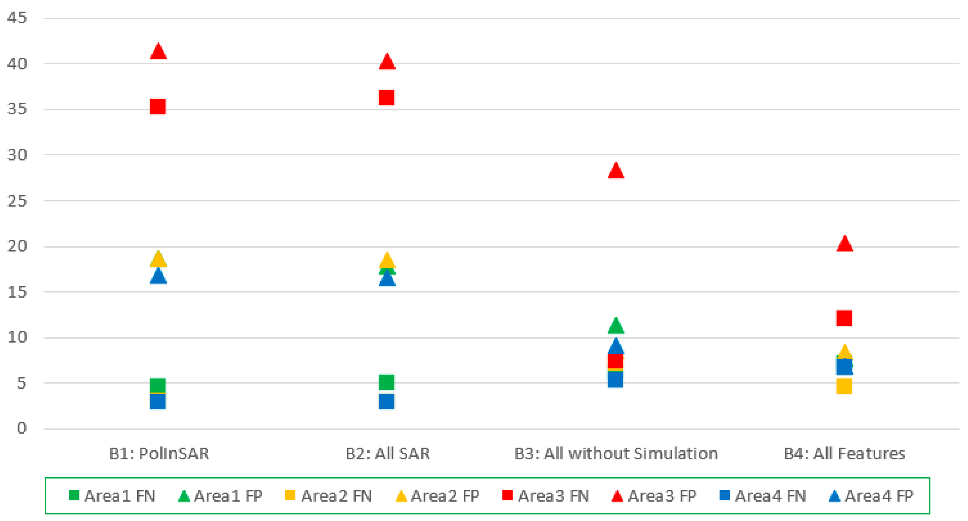
| Category | TP (%) | TN | FP | FN | TP | TN | FP | FN |
|---|---|---|---|---|---|---|---|---|
| Area1 | Area2 | |||||||
| B1 | 95.4 | 81.4 | 18.6 | 4.6 | 96.9 | 81.3 | 18.7 | 3.1 |
| B2 | 95 | 82.2 | 17.8 | 5 | 97.1 | 81.5 | 18.5 | 2.9 |
| B3 | 93.9 | 88.7 | 11.3 | 6.1 | 92.9 | 91.5 | 8.5 | 7.1 |
| B4 | 92.9 | 92.3 | 7.7 | 7.1 | 95.4 | 91.6 | 8.4 | 4.6 |
| Category | Area3 | Area4 | ||||||
| B1 | 64.8 | 58.5 | 41.5 | 35.2 | 97.1 | 83.1 | 16.9 | 2.9 |
| B2 | 63.8 | 59.6 | 40.4 | 36.2 | 97.1 | 83.5 | 16.5 | 2.9 |
| B3 | 92.6 | 71.6 | 28.4 | 7.4 | 94.7 | 90.9 | 9.1 | 5.3 |
| B4 | 87.9 | 79.7 | 20.3 | 12.1 | 93.3 | 93.1 | 6.9 | 6.7 |
| Proposed\Existing | SAR-Based Methods | Non-SAR-Based Method | ||
|---|---|---|---|---|
| A1: Intensity | A2: InSAR | A3: PolSAR | A5: Auxiliary | |
| B4: Incorporated PolInSAR, SAR Simulation, and Auxiliary Features | 7.1% | 10% | 6.3% | 9.7% |
| B2: PolInSAR and SAR Simulation | 3.4% | 6.5% | 2.7% | 6.1% |
Publisher’s Note: MDPI stays neutral with regard to jurisdictional claims in published maps and institutional affiliations. |
© 2022 by the authors. Licensee MDPI, Basel, Switzerland. This article is an open access article distributed under the terms and conditions of the Creative Commons Attribution (CC BY) license (https://creativecommons.org/licenses/by/4.0/).
Share and Cite
Baghermanesh, S.S.; Jabari, S.; McGrath, H. Urban Flood Detection Using TerraSAR-X and SAR Simulated Reflectivity Maps. Remote Sens. 2022, 14, 6154. https://doi.org/10.3390/rs14236154
Baghermanesh SS, Jabari S, McGrath H. Urban Flood Detection Using TerraSAR-X and SAR Simulated Reflectivity Maps. Remote Sensing. 2022; 14(23):6154. https://doi.org/10.3390/rs14236154
Chicago/Turabian StyleBaghermanesh, Shadi Sadat, Shabnam Jabari, and Heather McGrath. 2022. "Urban Flood Detection Using TerraSAR-X and SAR Simulated Reflectivity Maps" Remote Sensing 14, no. 23: 6154. https://doi.org/10.3390/rs14236154