Article

Storm-Time Relative Total Electron Content Modelling Using Machine Learning Techniques

by
Marjolijn Adolfs
1,2,*,
Mohammed Mainul Hoque
1 and
Yuri Y. Shprits
2,3,4
1
German Aerospace Center (DLR), Institute of Solar-Terrestrial Physics, Kalkhorstweg 53, 17235 Neustrelitz, Germany
2
Institute of Physics and Astronomy, University of Potsdam, 14476 Potsdam, Germany
3
Space Physics and Space Weather, Geophysics, GFZ German Research Centre for Geosciences, 14473 Potsdam, Germany
4
Department of Earth, Planetary and Space Sciences, University of California Los Angeles, Los Angeles, CA 90095, USA
*
Author to whom correspondence should be addressed.
Remote Sens. 2022, 14(23), 6155; https://doi.org/10.3390/rs14236155
Submission received: 27 October 2022 / Revised: 30 November 2022 / Accepted: 1 December 2022 / Published: 5 December 2022

Abstract

:
Accurately predicting total electron content (TEC) during geomagnetic storms is still a challenging task for ionospheric models. In this work, a neural-network (NN)-based model is proposed which predicts relative TEC with respect to the preceding 27-day median TEC, during storm time for the European region (with longitudes 30°W–50°E and latitudes 32.5°N–70°N). The 27-day median TEC (referred to as median TEC), latitude, longitude, universal time, storm time, solar radio flux index F10.7, global storm index SYM-H and geomagnetic activity index Hp30 are used as inputs and the output of the network is the relative TEC. The relative TEC can be converted to the actual TEC knowing the median TEC. The median TEC is calculated at each grid point over the European region considering data from the last 27 days before the storm using global ionosphere maps (GIMs) from international GNSS service (IGS) sources. A storm event is defined when the storm time disturbance index Dst drops below 50 nanotesla. The model was trained with storm-time relative TEC data from the time period of 1998 until 2019 (2015 is excluded) and contains 365 storms. Unseen storm data from 33 storm events during 2015 and 2020 were used to test the model. The UQRG GIMs were used because of their high temporal resolution (15 min) compared to other products from different analysis centers. The NN-based model predictions show the seasonal behavior of the storms including positive and negative storm phases during winter and summer, respectively, and show a mixture of both phases during equinoxes. The model’s performance was also compared with the Neustrelitz TEC model (NTCM) and the NN-based quiet-time TEC model, both developed at the German Aerospace Agency (DLR). The storm model has a root mean squared error (RMSE) of 3.38 TEC units (TECU), which is an improvement by 1.87 TECU compared to the NTCM, where an RMSE of 5.25 TECU was found. This improvement corresponds to a performance increase by 35.6%. The storm-time model outperforms the quiet-time model by 1.34 TECU, which corresponds to a performance increase by 28.4% from 4.72 to 3.38 TECU. The quiet-time model was trained with Carrington averaged TEC and, therefore, is ideal to be used as an input instead of the GIM derived 27-day median. We found an improvement by 0.8 TECU which corresponds to a performance increase by 17% from 4.72 to 3.92 TECU for the storm-time model using the quiet-time-model predicted TEC as an input compared to solely using the quiet-time model.

1. Introduction

Geomagnetic storms are disturbances in the Earth magnetosphere caused by enhancements in the solar wind by coronal mass ejections (CMEs) or high-speed solar-winds streams (HSS) [1,2,3]. Interactions of HSS with quiet-time solar wind cause corotating interaction regions (CIRs) [1] which cause geomagnetic storms. Coronal mass injections result from reconfigurations of the solar coronal magnetic field and injection of a magnetic cloud into the interplanetary fields. HSS originate from the coronal holes, where solar wind can escape more easily because of the Sun’s open magnetic field caused by temporary cooler, less dense regions [4]. During the declining phase of the solar cycle, coronal holes occur at lower latitudes and cause more frequent CIRs that can hit the Earth. CMEs have, in general, a higher occurrence during solar maximum [5] while some of the strongest CMEs have been, in fact, observed during the declining phase of the solar cycle. Geomagnetic storms can result in changes in the Earth’s magnetosphere which is two-way coupled to the ionosphere and can produce ionospheric disturbances due to electromagnetic flux heating and the precipitation of particles into the ionosphere. Total electron content (TEC) describes the line-of-sight number of charged particles in the ionosphere, and an increase in TEC corresponds to increasing propagation delays for transionospheric signals. The TEC can be represented by TEC units (TECU), where 1 TECU stands for 1016 free electrons/m2. The dispersive property of the ionosphere can be used to correct for the ionospheric delay by combining two or more frequencies. Single-frequency users, however, are not able to use multiple frequencies and need ionospheric models or external information to correct for this propagation effect [6,7,8]. Higher electron densities cause higher atmospheric drag on low orbiting satellites [9,10] and longer delays on Global Navigation Satellite Systems’ (GNSS) radio signals, which are used for navigation and other GNSS applications. Predicting TEC accurately during these space weather events is a challenging task, because during geomagnetic storms the TEC can dramatically change compared to the quiet-time conditions.
To show an example of how much the ionospheric TEC can be disturbed during a geomagnetic storm, the TEC relative to the 27-day median prior to the event (referred to as the relative TEC) can be used. The relative TEC is plotted in Figure 1 for the Halloween storms that occurred on 29 and 30 October 2003. The relative TEC is computed using the global ionosphere maps (GIMs) from the Universitat Politècnica de Catalunya (UPC) analysis center, downloaded from ftp://newg1.upc.es/upc_ionex/ (accessed on 8 May 2022). In this figure, we see that at certain locations the TEC can increase by more than 200% compared to the preceding 27-day median. Storms do not have to be short-lived phenomena but can have a duration that can last a few hours up to several days [11]. Therefore, it is important to predict ionospheric TEC accurately during disturbed periods as well.
There are neural-network (NN)-based approaches that also investigate the performance of TEC models during storm-time conditions. An NN-based TEC model, trained with data from a Peninsular Malaysia station from the years 2011 to 2014, was used by Akir et al. [12]. The performance of the TEC model was investigated during two geomagnetic storms in 2015. The study indicated that during major geomagnetic storms, the NN TEC model is unable to accurately predict the TEC. The model developed by Akir et al. [12] did not include any of the geomagnetic indices such as Kp, Hp, AE or Dst as input parameters. The Dst index describes the disturbance produced by the asymmetric ring current at low latitudes and the planetary Kp index measures global geomagnetic activity and is inferred from 13 mid-latitude stations. The NN storm-time TEC model over Sutherland, South Africa proposed by Uwamahoro and Habarulema [13] used the geomagnetic input parameter called A, which stands for the daily average level of geomagnetic activity. The model was trained with storm data from 1999 to 2013 and was not able to capture short-term storm features but could accurately predict storms with non-significant ionospheric TEC response and storms that occurred during low-solar-activity (LSA) conditions. The authors of [14] investigated the performance of the Nigerian total electron content (NIGTEC) regional NN-based model during two intense geomagnetic storms in March 2012 and 2013. NIGTEC used the disturbance index Dst as one of its input parameters and was able to capture the morphology of vertical TEC (VTEC) enhancement during the storm but not all storm-time related changes. The performance of several different long short-term memory (LSTM) network-based algorithms for global TEC predictions was investigated by Chen et al. [15]. The authors found that the multi-step-auxiliary-algorithm-based prediction model performed the best. The performance of the model was further validated with four geomagnetic storm events during 2020 (LSA conditions) and showed that the model has low error during a geomagnetic storm. A combination of LSTM, convolutional neural network (CNN) and attention mechanism for an ionospheric forecast model in China was used by Tang et al. [16]. The authors used the Dst, Kp and the magnetic-field southward component Bz as one of the input parameters. The network was tested with data from 2018, which was also a relatively quiet solar period (with an average F10.7 of 69.9 solar flux units).
The various NN-based approaches listed above use different algorithms for their storm-time TEC investigations. During our previous investigations in [17], we found that our FNN-based quiet-time model, developed at the German Aerospace Center (DLR), was capable of showing the small-scale nighttime winter anomaly feature of the ionosphere. The performance of the model deteriorates during storm time; this was also expected since the model does not include any geomagnetic indices as input parameters. Due to the model’s capability of providing predictions containing small-scale features of the ionosphere, the same algorithm was chosen to be used but now focused on storm-time conditions. The models discussed above predict the TEC directly but for the current study another method was chosen. Our work focuses on the prediction of TEC during storm time relative to the 27-day median of the preceding days, from now on referred to as the relative TEC. Predicting the relative TEC instead of the TEC directly, the model’s capability of capturing storm-related perturbations can be seen. The model can be applied using different data sources as well, which will be further explained in the Methods section. In this paper, an FNN model is proposed to predict the relative TEC for the European region (with longitudes 30°W–50°E and latitudes 32.5°N–70°N). The relative TEC is computed using TEC data from GIMs. There are eight Ionospheric Associate Analysis Centers (IAACs) under the International GNSS Service (IGS) that develop the GIMs [18,19]. The GIMs are provided in the ionosphere map exchange (IONEX) format. For this work, rapid UQRG GIMs are used, which have a 15-minute temporal resolution, released by the UPC analysis center. The spatial resolution is 5 degrees longitude by 2.5 degrees latitude. The UQRG GIMs are released with a one-day latency. The high temporal resolution makes these GIMs ideal to be used during storm events to capture small-scale storm-related changes.
The paper is divided into five sections, beginning with a brief description of different NN-based ionospheric TEC models and their capability of predicting TEC accurately during storms. Section 2 explains the database and sources needed for the model development. The method used for designing the storm-time NN-based model’s architecture is discussed in Section 3. Section 4 provides a performance evaluation of the storm-time NN model compared to an NN-based quiet-time model [17] and the Neustrelitz TEC model (NTCM) [20], which is a computationally very fast 12-coefficient model that uses the daily solar flux F10.7 as a driving parameter. The storm-time NN-based model is further evaluated with respect to its capability of predicting TEC using the quiet-time model outputs as an input for the storm-time model in order to improve the quiet-time model’s accuracy. The conclusions are given in Section 5.

2. Database

A storm dataset was needed for this study in order to train and test the model. The dataset contains storms occurring in the time period from 1998 until 2020. The geomagnetic storm-time disturbance index Dst was used to detect storms because it is, according to Wanliss and Showalter, “the most widely used statistical descriptor of space storm activity” [21] and commonly used for storm classifications. In Figure 2, the Dst and SYM-H index, which can be used as a high-resolution Dst index [21], are plotted during a storm that occurred 7–10 December 2013. According to Gonzalez et al. [22], storms can be classified as follows: −50 ≤ Dst ≤ −30 as weak, −100 ≤ Dst ≤ −50 as moderate and Dst ≤ −100 as intense storms. In our study, we classified occurrences as storms if the Dst became lower than −50 nanotesla (nT). The onset time (storm time = 0) was defined as the time of maximum Dst right before the index started decreasing [23], shown as the dashed black line in Figure 2.
It is worth noting that the storm onset of magnetic storms is characterized by increases in magnetic field strength, sudden impulses (SIs) and storm sudden commencements (SSCs). Therefore, the true onset of the magnetic storm in Figure 2 is the rise time before the “ST = 0”. However, for simplicity, we considered the onset as the time of maximum Dst before the decreasing Dst values [23]. We assume that since we are using TEC data of either 15-min or 1-h time resolutions, the difference in true onset and considered onset will not impact the TEC modelling performance.
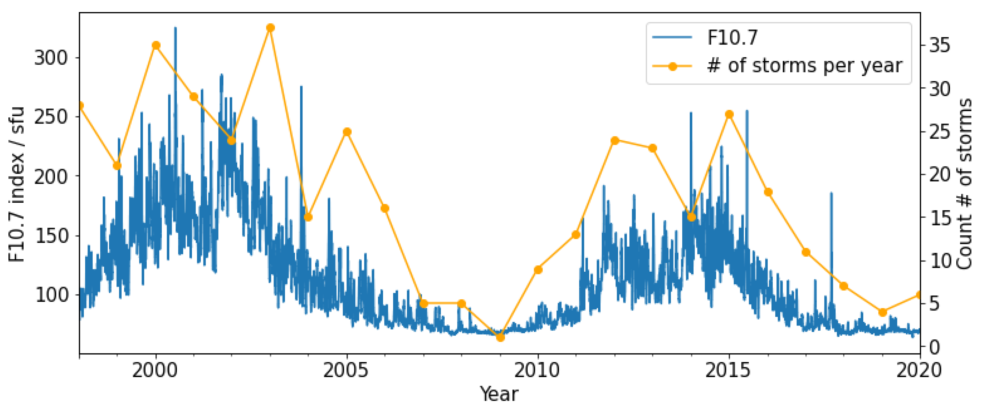
In total, there were 398 storms identified during the investigated time period. Most storms occurred during high-solar-activity (HSA) periods, as shown below in Figure 3, where the daily solar flux F10.7 is plotted together with the number of storms for each year.
We used the relative TEC in order to analyse and model storm-related perturbations, defined in the Equation (1) below.
Relative TEC = T E C T E C 27 d a y m e d i a n T E C 27 d a y m e d i a n · 100 %
In some cases, the median TEC was zero; here, we decided to calculate the relative TEC by substituting the median using a nominal value. The nominal value is 1 TECU during daytime, which is from 6 until 18 universal time (UT), and 0.5 TECU during nighttime, this way, a division by zero is prevented. The nominal values are assumed from our long-term experiences on TEC reconstruction and modelling [20,24,25,26]. The storms were divided into seasons according to their day of year (DOY). This is shown in Table 1, below, together with the number of storms for each season. The DOY used to classify the storms into seasons, listed in Table 1, corresponds to the following months: winter season storms occurred from November until February, summer storms from May until August and equinox storms during March, April, September and October.
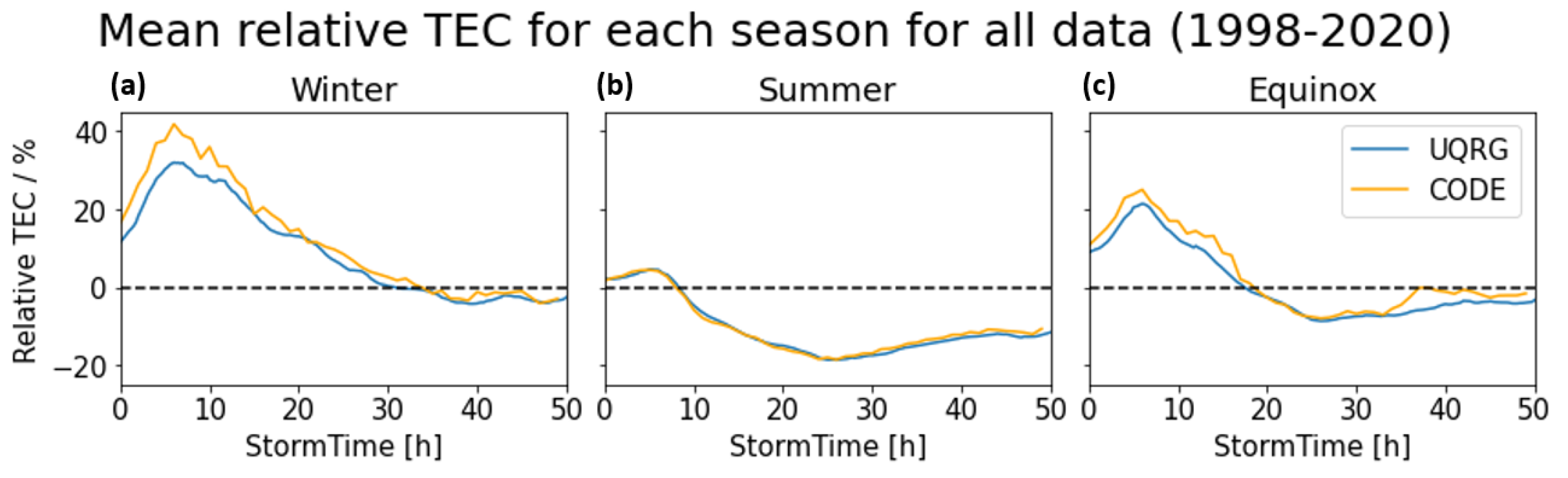
In Figure 4, the relative TEC as a function of storm time (averaged over the complete region) is plotted during each season for UQRG data from UPC and data from the Center for Orbit Determination in Europe (CODE) analysis center. A comparison with data from CODE was made in order to see if the same storm-related perturbations are visible in both datasets. In general, the relative TEC for CODE and UQRG data is very similar but for the winter and equinox storms, a small increase at the beginning of the storm is seen for the CODE relative TEC. This can be partially explained by the differences in temporal resolution between the GIMs, which can result in more extreme peaks because there are fewer data points. However, this does not justify why it only occurs within the positive relative TEC phases and is not seen during summer storms, where negative phases are stronger. From the plots in Figure 4, a strong positive phase (i.e., TEC increase relative to 27-day median) during winter storms can be seen where the summer storms have a negative phase. The equinox storms look like a mixture of the other two seasons. A seasonal effect was also found in [23,27,28,29], where during winter storms the positive phase of TEC is dominant and during summer the decreasing effect is dominant.
The rapid UQRG GIMs provided by UPC were downloaded from ftp://newg1.upc.es/upc_ionex/ (accessed on 8 May 2022). The geomagnetic conditions are described by the global storm index also known as disturbance index SYM-H and the geomagnetic activity index Hp30. The SYM-H index was chosen instead of the disturbance index Dst as an input parameter because it has a 1-minute time resolution [21]. SYM-H was downloaded from http://wdc.kugi.kyoto-u.ac.jp/aeasy/index.html (accessed on 10 March 2022). The high-cadence Hp30 index is a high-resolution Kp index [30,31] and can be accessed at https://www.gfz-potsdam.de/en/hpo-index/ (accessed on 10 March 2022). The Hp30 has a 30-min time resolution, whereas the Kp index has a 3-h time resolution. Both SYM-H and Hp30 indices have been linearly interpolated to a time resolution of 15 min, equal to the UQRG GIMs.

3. Method

In case of the NN-based quiet-time model [17], the DOY, UT, geomagnetic latitude, geographic longitude, solar zenith angle and solar radio flux index F10.7 were used as input parameters. Studies [13,14,15,16] have shown that other NN-based models considered geomagnetic indices as inputs as well. Therefore, for the storm-time model, we considered the same input parameters as the quiet-time model (except for the geomagnetic latitude and the solar zenith angle) together with new inputs such as the storm time (where the storm time = 0 corresponds to the time of maximum Dst right before the Dst starts decreasing), 27-day median TEC of the preceding days and the geomagnetic indices SYM-H and Hp30. Including the storm time as an input parameter, the model could capture the timing of the positive or negative relative TEC phases of the storms better. Since, during this study, the rapid UQRG GIMs were used, there is a latency of one day before the GIMs become available. Therefore, the 27-day median can be computed without complications in the lag time of the release of the GIMs. Adding the solar zenith angle as an input did not improve the accuracy of the model and, therefore, it was not included. The solar zenith angle does not change very much because the model is limited to the European region. This is also the reason why the geographic latitude was used instead of the geomagnetic latitude. Other indices besides the Hp30 and SYM-H, e.g., Bz component of planetary magnetic field, solar-wind flow speed, solar-wind pressure and proton density were also investigated to check whether they would improve the accuracy of the model or not. The indices were downloaded from the OMNIWeb interface, available at https://omniweb.gsfc.nasa.gov/form/dx1.html (accessed on 10 March 2022). Using the Bz, solar-wind flow speed, solar-wind pressure and proton density as input parameters did not improve the accuracy of the network. The temporal resolution of these parameters provided by the OMNIWeb database is 1-h, which may not be sufficient to describe the small-scale perturbations seen in the relative TEC computed with the UQRG GIMs, which have a temporal resolution of 15-min. Finally, the following inputs were selected to train the neural network with: SYM-H, Hp30, DOY, UT, storm time, solar flux index F10.7 and the 27-day median TEC of the preceding days. The features and the correct set of hyperparameters were selected by training different models and comparing the training and validation loss and accuracy. Future selection may be also performed in an automated way using various machine-learning methods such as random forests, mutual information or fast function extraction [32].
The data was divided into training, validation and testing datasets. It was divided by year in order to avoid information leakage, where the model already has information about the test dataset and predictions during testing become too optimistic. This can occur when the dataset contains very short intervals of data instead of complete storms or when a scaler for normalization is also fitted on the testing data. Using the training and validation datasets, the free parameters, also known as hyperparameters, are optimized. A few examples of the different hyperparameters that have to be set are the number of neurons or layers, activation function, regularization, learning rate and optimizer. The validation set was about 20 percent of the training dataset. The testing dataset consists of a total of 33 storms that happened during 2015 (27 storms), which is an HSA period, and 2020 (6 storms), an LSA period. The testing dataset is excluded from the training and validation datasets, which means that the data is unseen until the performance of the model is tested. Early stopping, where the model stops the training process when the validation loss does not decrease for a certain number of epochs, was used so that the model does not overfit the training data and to reduce training time. The data was normalized using the MinMaxScaler function from the Scikit-Learn Python library [33] to a range of [0, 1] and fitted on the training and validation datasets. Using normalized data, the model can converge faster. The FNN is built with Tensorflow [34] and Keras Python libraries [35]. To map non-linearities, the rectified linear unit (ReLU) was chosen as an activation function for the hidden layer, which is a very popular non-linear activation function [36]. The output layer uses the linear identity activation function. Optimization algorithm ’Adam’ was used, which minimizes the mean squared error and is a computationally effective algorithm with low memory requirements [37]. A learning rate of 0.0001 was used for the Adam optimizer. To avoid overfitting, a regularization term can be added which penalizes the model for fitting the training data too well. Therefore, a small regularization term of 0.00004 was added to the network.
The results for training the models with different numbers of neurons in one hidden layer are plotted in Figure 5. In this figure, the results in terms of root mean square error (RMSE) and correlation for the relative TEC and the TEC are displayed. The relative TEC is converted to TEC in order to also show how well the model is performing in terms of TECU. This figure shows that the correlation increases and the RMSE decreases when more neurons are used in the hidden layer. Deeper networks, with architectures similar to the investigations carried out by Orus Perez [38], were tested but the accuracy did not increase when more layers were used, as shown in Table 2 below. After testing different architectures and hyperparameters, a network architecture with one hidden layer containing 40 neurons was chosen. The general architecture of the NN is shown Figure 6. After choosing the hyperparameters and features, the model was trained once more with the validation data included. The model was trained on a personal computer with an Intel Core i7-8665U CPU and 16 GB RAM; therefore, no special hardware was needed. The model was fitted in 30 epochs (the number of cycles that the complete training dataset passes through the network) using a batch size (number of samples that are propagated through the network) of 128.
The model predicts the relative TEC, and the TEC is computed using the 27-day median of the preceding days. The TEC was computed using Equation (2).
T E C = Relative TEC · T E C 27 d a y m e d i a n 100 + T E C 27 d a y m e d i a n
In this study, we also investigated if the quiet-time model VTEC predictions could be used as a substitute for the input of the 27-day median TEC. The quiet-time model was trained with Carrington-rotation-averaged TEC data, which is approximately 27 days. Using the output of the quiet-time model instead of the 27-day median, the relative TEC was predicted. The predicted relative TEC was used to update the quiet-time VTEC predictions in order to see if the quiet-time model was then capable of capturing the storm-time perturbations better. An overview of the method is shown in Figure 7, below. The magnetic latitude, used for the quiet-time model, was not used for the storm-time model but the geographic latitude was used instead.
The performance of the model was tested by comparing the model’s predictions with the NTCM and the quiet-time model. The computationally very fast 12 coefficient NTCM developed at DLR is comparable in its simplicity to the GPS Klobuchar model and achieves a similar performance as the NeQuick G (optimized for Galileo system) and was recently adopted by the European Commission as an alternative to the NeQuick G model [20,24,25,26]. The results are shown in the section below.

4. Results and Discussion

To validate the storm-time model, a comparison with the NTCM and quiet-time model was made. The storm-time model was also coupled with the quiet-time model using the quiet-time TEC predictions as a substitute of the median TEC in order to see if it can increase the quiet-time model’s accuracy during storms. After the comparisons, the performance of the model was investigated by comparing the predictions of the model at each grid point with the GIMs and by analyzing the RMSE for each of the input features of the model.

4.1. Comparison between NTCM and Quiet-Time Model

To validate the model, the performance of the storm model was compared to the performance of the NTCM and the quiet-time NN-based global TEC model. The performance of the models in terms of mean and standard deviation (STD) are shown in Figure 8, below, and an overview of the RMSE is displayed in Table 3. The quiet-time model was trained with CODE GIMs and has a performance of 4.67 TECU when CODE data was used as the true value. When UQRG data was used instead of CODE as true value, the performance of the model is 4.72 TECU, which is slightly worse but not a significant difference (0.05 TECU). Therefore, the UQRG GIMs were used as the true value for all models. The histograms were computed by subtracting the predictions of the storm-time, NTCM and quiet-time model from the true value. The storm model has an overall RMSE of 3.38 TECU, which is an improvement by 1.87 TECU (35.6%) compared to the NTCM, which has an RMSE of 5.25 TECU. The storm model outperformed the quiet-time model by 1.34 TECU which corresponds to a performance increase by 28.4% from 4.72 to 3.38 TECU. From Figure 8, it becomes clear that all models perform better during the LSA year 2020, which is as expected. The difference in performance between the three models during that year is very small, e.g., the RMS residual is approximately 0.7 and 1 TECU less for of the storm-time model compared to the quiet model and NTCM, respectively. The performance of the storm model becomes more significant during the HSA year 2015, which is also the period where the most storms occurred during the last solar cycle.
In Figure 9, the relative TEC as a function of storm time (averaged over the complete region) is plotted with the quiet- and storm-time model predictions for the test dataset, which contains storms during 2015 and 2020. The quiet-time model does not show any storm-related perturbations, which was also expected because the model is not driven by geomagnetic indices. The relative TEC calculated with predictions from the quiet-time model are showing negative percentages. A reason for this behaviour may be that the 27-day median from UQRG GIMs, which are used to compute the relative TEC, are slightly higher than CODE data, causing these negative percentages. The storm-time model shows a positive phase during the winter storms and summer storms have a negative phase. The equinox storms look like a mixture of both of them.

4.2. Using Quiet-Time Model as Input for Storm-Time Model

The quiet-time model is not able to show storm-related perturbations. Therefore, the storm model is coupled with the quiet-time model in order to increase the quiet-time model performance during storms. Applying the quiet-time model as an input for the storm-time model’s median TEC, the accuracy of the predictions improves by approximately 0.8 TECU compared to solely using the quiet-time model. This corresponds to a performance increase by 17% from 4.72 to 3.92 TECU. To visualize the improvement achieved using a combination of the quiet- and storm-time model, the TEC (blue line) and predictions of the quiet-time model (orange line), storm-time model (green line) and storm-time model combined with the quiet-time model (red line) during two storms were plotted along with the SYM-H index in Figure 10. In the left panel, an improvement by 2.94 TECU, which corresponds to a performance increase by 30.9% from 9.52 to 6.58 TECU, is seen when the storm model is coupled with the quiet-time model compared to solely using the quiet-time model. If the storm model uses the 27-day median TEC from UQRG data as an input instead of the predictions of the quiet-time model, the difference between TEC and predictions becomes even smaller (green line), but this is not the case for all storms. In the right panel, the same was plotted but during a different storm. In these plots, comparing the red and green curves, the difference is smaller between the storm model using the 27-day median obtained from the UQRG GIMs as an input and the storm model which is coupled with the quiet-time model. Applying the quiet-time-modelled TEC as input to the storm model during this storm improves the predictions by 3.18 TECU, which corresponds to a performance increase by 50.8% from 6.26 to 3.08 TECU, compared to the quiet-time model.

4.3. Performance Analysis: Storm Model

To investigate the performance of the storm model further, the RMSE and correlation for each season is provided, as shown in Table 4. The storm-time model performs the best in terms of RMSE and correlation in the case of summer storms. During winter storms, a higher RMSE is seen and equinox storms have the lowest correlation for the relative TEC. The same behaviour is seen in Figure 11, where the relative TEC is plotted for the European region averaged for all storms in the test dataset (2015 and 2020) and divided by each season according to the DOY listed in Table 1. In this figure, the top panel shows the mean relative TEC from the GIMs, the middle panel shows the predictions and the bottom panel shows the difference between the model and the GIMs. The differences are computed by subtracting the GIMs relative TEC from the predictions. From this figure, we can see that the model is over-predicting in the winter season in the northern latitudes. During equinox storms, the model is generally over-predicting in the whole European region. The model is under-predicting during summer storms and also winter storms, but in case of winter storms only for lower latitudes with western longitudes.
The RMSE was also plotted against different parameters, e.g., the storm time, local time, DOY, SYM-H, Hp30, F10.7, longitude and latitude, for all the storms from the test dataset, which is shown in Figure 12. Looking at the top left panel, we see that the storm-time model is less accurate during the first part of the storm. As the storm continues, the model becomes more accurate. This was expected because the storms have the largest changes in TEC during the first part of the storm, as also shown in Figure 4 (in the case of winter and equinox storms). The top right panel shows the RMSE for each local time (LT). The lowest RMSE is seen in the morning hours with the minimum at 7–8 LT. The lack of sunlight (lower TEC levels) during the night can explain why the RMSE is dropping and when the sun rises, the ionosphere becomes more active, causing the higher RMSE values during these hours. This only partially explains the RMSE behaviour because the RMSE keeps increasing even though the sun sets in the evening and finally starts decreasing around midnight. From the plot where the RMSE is plotted against DOY, it can be seen that the model performs better during the summer, which is also observed in Figure 9 and in Table 4. As expected, the SYM-H and Hp30 plots show that the accuracy of the model deteriorates when the storms become stronger. The F10p7 plot suggests that higher solar activity does not cause a large difference in prediction errors of the relative TEC. The longitude plot shows a minimum of RMSE at around 30 degree east and the latitude plot shows a minimum at around 55 degree north, but the range is very small.
The general performance of the model is good but the model’s performance can differ for each storm. A reason for this kind of behavior may be that the storms are very different from each other and, therefore, the model cannot predict all of them with the same accuracy. In this paper, an FNN architecture was used to model the storms; this way, the performance could be fairly compared to the quiet-time NN model which used the same architecture. Other NN architectures should also be investigated in the future, e.g., the LSTM architecture.

5. Conclusions

In this work, a storm-time NN-based relative TEC model for the European region (with longitudes 30°W–50°E and latitudes 32.5°N–70°N) was proposed. The model uses the SYM-H, Hp30, DOY, UT, storm time, solar flux index F10.7 and the 27-day median TEC as input parameters in order to predict the relative TEC. The model was trained with UQRG GIM data from the UPC analysis center during storms. The storm dataset contains storms during the period 1998–2019, with the year 2015 excluded. The years 2015 and 2020 were used for testing which are a high-solar-activity and low-solar-activity year, respectively.
The method used for this paper provides the relative TEC with respect to the 27-day median TEC prior to the storm as an output instead of predicting the TEC directly. The 27-day median TEC of the preceding days computed from GIMs or TEC models can be provided as input.
Our investigations show that the model can describe the vertical TEC behavior during storm time well in many cases. The predicted relative TEC shows seasonal behavior, e.g., stronger positive phases during winter and negative phases during summer months. The performance of the model was compared to the quiet-time NN-based TEC model and the NTCM. The storm model outperformed the NTCM by approximately 1.9 TECU, which corresponds to a performance increase by 35.6% from 5.25 to 3.38 TECU. The storm-time model outperforms the quiet-time model by 1.3 TECU, which corresponds to a performance increase by 28.4% from 4.72 to 3.38 TECU. The model was also tested for whether it is capable of improving the quiet-time model performance, because the quiet-time model does not show storm-related perturbations. For this, the output of the quiet-time model was used as an input to the storm-time model, substituting the 27-day median TEC. The relative TEC was then computed and used to calculate the TEC. This method could improve the quiet-time model TEC predictions by 0.8 TECU, which corresponds to a performance increase by 17% from 4.72 to 3.92 TECU.

Author Contributions

Conceptualization, M.A. and M.M.H.; methodology, M.A. and M.M.H.; software, M.A.; formal analysis, M.A. and M.M.H.; visualization, M.A.; writing—original draft preparation, M.A.; writing—review and editing, M.A., M.M.H. and Y.Y.S.; supervision, M.M.H. and Y.Y.S.; funding acquisition, M.M.H. All authors have read and agreed to the published version of the manuscript.

Funding

This research was funded by the German Research Foundation (DFG) under Grant No. HO 6136/1-1 and by the ‘Helmholtz Pilot Projects Information & Data Science II’ (grant support from the Initiative and Networking Fund of the Hermann von Helmholtz Association Deutscher Forschungszentren e.V. (ZT-I-0022)) with the project named ‘MAchine learning based Plasma density model’ (MAP).

Data Availability Statement

Not applicable.

Acknowledgments

The authors would like to thank the IGS and UPC for providing the GIM products, available at: https://cddis.nasa.gov/archive/gnss/products/ionex/ and ftp://newg1.upc.es/upc_ionex/ (accessed on 8 May 2022). The authors would also like to thank GSFC/SPDF OMNIWeb interface for the OMNI data, available at: https://omniweb.gsfc.nasa.gov (accessed on 10 March 2022).

Conflicts of Interest

The authors declare no conflict of interest. The funders had no role in the design of the study; in the collection, analyses, or interpretation of data; in the writing of the manuscript; or in the decision to publish the results.

References

  1. Zhang, J.; Richardson, I.G.; Webb, D.F.; Gopalswamy, N.; Huttunen, E.; Kasper, J.C.; Nitta, N.V.; Poomvises, W.; Thompson, B.J.; Wu, C.C.; et al. Solar and interplanetary sources of major geomagnetic storms (Dst ≤ −100 nT) during 1996–2005. J. Geophys. Res. Space Phys. 2007, 112, A10102. [Google Scholar] [CrossRef] [Green Version]
  2. Patel, K.; Singh, A.; Singh, S.B.; Singh, A.K. Causes responsible for intense and severe storms during the declining phase of Solar Cycle 24. J. Astrophys. Astron. 2019, 40, 4. [Google Scholar] [CrossRef]
  3. Brueckner, G.E.; Delaboudiniere, J.P.; Howard, R.A.; Paswaters, S.E.; St. Cyr, O.C.; Schwenn, R.; Lamy, P.; Simnett, G.M.; Thompson, B.; Wang, D. Geomagnetic storms caused by coronal mass ejections (CMEs): March 1996 through June 1997. Geophys. Res. Lett. 1998, 25, 3019–3022. [Google Scholar] [CrossRef]
  4. Gonzalez, W.D.; Tsurutani, B.T.; Clúa de Gonzalez, A.L. Interplanetary origin of geomagnetic storms. Space Sci. Rev. 1999, 88, 529–562. [Google Scholar] [CrossRef]
  5. Alves, M.V.; Echer, E.; Gonzalez, W.D. Geoeffectiveness of corotating interaction regions as measured by Dst index. J. Geophys. Res. Space Phys. 2006, 111, A7. [Google Scholar] [CrossRef] [Green Version]
  6. Klobuchar, J.A. Ionospheric Time-Delay Algorithm for Single-Frequency GPS Users. IEEE Trans. Aerosp. Electron. Syst. 1987, AES-23, 325–331. [Google Scholar] [CrossRef]
  7. Bidaine, B.; Lonchay, M.; Warnant, R. Galileo single frequency ionospheric correction: Performances in terms of position. GPS Solut. 2013, 17, 63–73. [Google Scholar] [CrossRef] [Green Version]
  8. Yuan, Y.; Wang, N.; Li, Z.; Huo, X. The BeiDou global broadcast ionospheric delay correction model (BDGIM) and its preliminary performance evaluation results. NAVIGATION 2019, 66, 55–69. [Google Scholar] [CrossRef] [Green Version]
  9. Walterscheid, R.L. Solar cycle effects on the upper atmosphere—Implications for satellite drag. J. Spacecr. Rocket. 1989, 26, 439–444. [Google Scholar] [CrossRef]
  10. Chen, G.; Xu, J.; Wang, W.; Lei, J.; Burns, A.G. A comparison of the effects of CIR- and CME-induced geomagnetic activity on thermospheric densities and spacecraft orbits: Case studies. J. Geophys. Res. Space Phys. 2012, 117. [Google Scholar] [CrossRef]
  11. Davies, K. Ionospheric Radio; The Institution of Engineering and Technology: London, UK, 1990; pp. 331–333. [Google Scholar]
  12. Akir, R.M.; Bahari, S.A.; Abdullah, M.; Homam, M.J.; Chellapan, K.; Ngadengon, R. Forecasting Ionospheric Total Electron Content During Geomagnetic Storms. In Proceedings of the 2020 IEEE Student Conference on Research and Development (SCOReD), Batu Pahat, Malaysia, 27–29 September 2020; pp. 1–6. [Google Scholar] [CrossRef]
  13. Uwamahoro, J.C.; Habarulema, J.B. Modelling total electron content during geomagnetic storm conditions using empirical orthogonal functions and neural networks. J. Geophys. Res. Space Phys. 2015, 120, 11000–11012. [Google Scholar] [CrossRef]
  14. Amaechi, P.O.; Humphrey, I.; Adewoyin, D.A. Assessment of the predictive capabilities of NIGTEC model over Nigeria during geomagnetic storms. Geod. Geodyn. 2021, 12, 413–423. [Google Scholar] [CrossRef]
  15. Chen, Z.; Liao, W.; Li, H.; Wang, J.; Deng, X.; Hong, S. Prediction of Global Ionospheric TEC Based on Deep Learning. Space Weather 2022, 20, e2021SW002854. [Google Scholar] [CrossRef]
  16. Tang, J.; Li, Y.; Ding, M.; Liu, H.; Yang, D.; Wu, X. An Ionospheric TEC Forecasting Model Based on a CNN-LSTM-Attention Mechanism Neural Network. Remote Sens. 2022, 14, 2433. [Google Scholar] [CrossRef]
  17. Adolfs, M.; Hoque, M.M. A Neural Network-Based TEC Model Capable of Reproducing Nighttime Winter Anomaly. Remote Sens. 2021, 13, 4559. [Google Scholar] [CrossRef]
  18. Ogwala, A.; Oyedokun, O.J.; Ogunmodimu, O.; Akala, A.O.; Ali, M.A.; Jamjareegulgarn, P.; Panda, S.K. Longitudinal Variations in Equatorial Ionospheric TEC from GPS, Global Ionosphere Map and International Reference Ionosphere-2016 during the Descending and Minimum Phases of Solar Cycle 24. Universe 2022, 8, 575. [Google Scholar] [CrossRef]
  19. Panda a, S.K.; Harikaa, B.; Vineetha, P.; Kumar Dabbakutib, J.R.K.; Akhila, S.; Srujanaa, G. Validity of Different Global Ionospheric TEC Maps over Indian Region. In Proceedings of the 2021 3rd International Conference on Advances in Computing, Communication Control and Networking (ICAC3N), Greater Noida, India, 17–18 December 2021; pp. 1749–1755. [Google Scholar] [CrossRef]
  20. Jakowski, N.; Hoque, M.M.; Mayer, C. A new global TEC model for estimating transionospheric radio wave propagation errors. J. Geod. 2011, 85, 965–974. [Google Scholar] [CrossRef]
  21. Wanliss, J.A.; Showalter, K.M. High-resolution global storm index: Dst versus SYM-H. J. Geophys. Res. Space Phys. 2006, 111, A2. [Google Scholar] [CrossRef]
  22. Gonzalez, W.D.; Joselyn, J.A.; Kamide, Y.; Kroehl, H.W.; Rostoker, G.; Tsurutani, B.T.; Vasyliunas, V.M. What is a geomagnetic storm? J. Geophys. Res. Space Phys. 1994, 99, 5771–5792. [Google Scholar] [CrossRef] [Green Version]
  23. Borries, C.; Berdermann, J.; Jakowski, N.; Wilken, V. Ionospheric storms-A challenge for empirical forecast of the total electron content. J. Geophys. Res. Space Phys. 2015, 120, 3175–3186. [Google Scholar] [CrossRef]
  24. Hoque, M.M.; Jakowski, N.; Berdermann, J. Ionospheric correction using NTCM driven by GPS Klobuchar coefficients for GNSS applications. GPS Solut. 2017, 21, 1563–1572. [Google Scholar] [CrossRef]
  25. Hoque, M.M.; Jakowski, N.; Berdermann, J. Positioning performance of the NTCM model driven by GPS Klobuchar model parameters. J. Space Weather Space Clim. 2018, 8, A20. [Google Scholar] [CrossRef] [Green Version]
  26. Hoque, M.M.; Jakowski, N.; Orús-Pérez, R. Fast ionospheric correction using Galileo Az coefficients and the NTCM model. GPS Solut. 2019, 23, 41. [Google Scholar] [CrossRef]
  27. Blagoveshchensky, D.V.; Maltseva, O.A.; Sergeeva, M.A. Impact of magnetic storms on the global TEC distribution. Ann. Geophys. 2018, 36, 1057–1071. [Google Scholar] [CrossRef] [Green Version]
  28. Kil, H.; Paxton, L.J.; Pi, X.; Hairston, M.R.; Zhang, Y. Case study of the 15 July 2000 magnetic storm effects on the ionosphere-driver of the positive ionospheric storm in the winter hemisphere. J. Geophys. Res. Space Phys. 2003, 108, A11. [Google Scholar] [CrossRef]
  29. Titheridge, J.E.; Buonsanto, M.J. A comparison of northern and southern hemisphere TEC storm behaviour. J. Atmos. Terr. Phys. 1988, 50, 763–780. [Google Scholar] [CrossRef]
  30. Matzka, J.; Bronkalla, O.; Kervalishvili, G.; Rauberg, J.; Stolle, C. Geomagnetic Hpo Index, 2021. V. 1.0. GFZ Data Services. Available online: https://dataservices.gfz-potsdam.de/panmetaworks/showshort.php?id=7d8f890c-9852-11eb-9603-497c92695674 (accessed on 10 March 2022).
  31. Kervalishvili, G.; Matzka, J.; Stolle, C.; Rauberg, J. The open-ended, high cadence, Kp-like geomagnetic Hp30 and Hp60 indices. In Proceedings of the EGU General Assembly 2021, Online, 19–30 April 2021. EGU21-2846. [Google Scholar] [CrossRef]
  32. Zhelavskaya, I.S.; Vasile, R.; Shprits, Y.Y.; Stolle, C.; Matzka, J. Systematic Analysis of Machine Learning and Feature Selection Techniques for Prediction of the Kp Index. Space Weather 2019, 17, 1461–1486. [Google Scholar] [CrossRef]
  33. Pedregosa, F.; Varoquaux, G.; Gramfort, A.; Michel, V.; Thirion, B.; Grisel, O.; Blondel, M.; Prettenhofer, P.; Weiss, R.; Dubourg, V.; et al. Scikit-learn: Machine Learning in Python. J. Mach. Learn. Res. 2011, 12, 2825–2830. [Google Scholar]
  34. Abadi, M.; Agarwal, A.; Barham, P.; Brevdo, E.; Chen, Z.; Citro, C.; Corrado, G.S.; Davis, A.; Dean, J.; Devin, M.; et al. TensorFlow: Large-Scale Machine Learning on Heterogeneous Systems. 2015. Available online: tensorflow.org (accessed on 10 March 2022).
  35. Chollet, F. Keras. 2015. Available online: https://keras.io (accessed on 10 March 2022).
  36. LeCun, Y.; Bengio, Y.; Hinton, G. Deep learning. Nature 2015, 521, 436–444. [Google Scholar] [CrossRef]
  37. Kingma, D.P.; Ba, J. Adam: A Method for Stochastic Optimization. arXiv 2014, arXiv:1412.6980. [Google Scholar]
  38. Orús Pérez, R. Using TensorFlow-based Neural Network to estimate GNSS single frequency ionospheric delay (IONONet). Adv. Space Res. 2019, 63, 1607–1618. [Google Scholar] [CrossRef]
Figure 1. The relative total electron content (TEC) with respect to the preceding 27-day median (calculated according to Equation (1)) for the Halloween storms that occurred on 29 and 30 October 2003. The relative TEC is calculated using the UQRG global ionosphere maps (GIMs) from the Universitat Politècnica de Catalunya (UPC) analysis center. The main phase of the storms was on 29 and 30 October, which are day of year (DOY) 302 and 303, respectively. The recovery phase lasted several days, until 3–4 November 2003. The relative TEC percentages are plotted at 22 universal time (UT) for 29–31 October, which corresponds to DOY 302 (a), 303 (b) and 304 (c), respectively.
Remotesensing 14 06155 g001
Figure 2. The geomagnetic storm time disturbance index Dst plotted together with the SYM-H index during a geomagnetic storm that occurred on 7–9 December 2013. The storm’s onset time (the time where maximum Dst is seen right before it starts decreasing), which corresponds to storm time = 0, is plotted as the dashed black line.
Remotesensing 14 06155 g002
Figure 3. F10.7 solar flux index plotted together with the number (#) of storms counted for each year for the complete dataset which contains storms occurring in the time period from 1998 until 2020.
Remotesensing 14 06155 g003
Figure 4. Comparison of the relative TEC between the UQRG from UPC and Center for Orbit Determination in Europe (CODE) GIM data as a function of storm time (averaged over the complete region) plotted for winter (a), summer (b) and equinox (c). The classification into seasons was performed according to the DOY listed in Table 1. Storm time equals zero corresponds to the time where the Dst index was maximum, right before it started decreasing.
Remotesensing 14 06155 g004
Figure 5. The number (#) of neurons in the hidden layer plotted against the root mean square error (RMSE), shown with the blue line, and the correlation (orange line) for the relative TEC (a) as a percentage and the TEC (b) in TEC Units (TECU).
Remotesensing 14 06155 g005
Figure 6. General overview of the neural network (NN) architecture where ST stands for the storm time and med-TEC for the 27-day median of the preceding days before the storm.
Remotesensing 14 06155 g006
Figure 7. An overview of how the storm-time model is coupled with the quiet-time model. The quiet-time model’s vertical TEC (VTEC) predictions are used as a substitute for the 27-day median TEC.
Remotesensing 14 06155 g007
Figure 8. The performance of the storm model, quiet-time model and Neustrelitz TEC model (NTCM) in TECU. The left panels (a,c) correspond to the high-solar-activity (HSA) year in 2015 and the right panels (b,d) to the low-solar-activity (LSA) year in 2020.
Remotesensing 14 06155 g008
Figure 9. The performance of the quiet-time and the storm-time model in relative TEC as a function of storm time (averaged over complete region) for the test data set (2015 and 2020) during winter (a), summer (b) and equinox (c). The classification into seasons was performed according to the DOY listed in Table 1.
Remotesensing 14 06155 g009
Figure 10. In the top panel is the UQRG TEC (blue curve) plotted together with the predicted TEC by the quiet-time model (orange curve), storm-time model (green curve) and the storm-time model coupled with the quiet-time model (red curve) for a geomagnetic storm on 17 February 2015 (a) with the SYM-H index plotted at the same time (b). The same is plotted for another storm that occurred on 11 May 2015, shown in (c) together with the corresponding SYM-H index (d).
Remotesensing 14 06155 g010
Figure 11. The relative TEC for the European region averaged for all storms in the test dataset (storms during 2015 and 2020) from the GIMs in panel (a), the predictions in panel (b) and the difference maps in (c). The difference maps were computed by subtracting the GIMs relative TEC from the predictions. The classification into seasons was performed according to the DOY listed in Table 1. The top colour bar corresponds to panel (a,b). The colour bar in the bottom to panel (c).
Remotesensing 14 06155 g011
Figure 12. The RMSE of the relative TEC plotted for different parameters which are the storm time (a), local time (b), DOY (c), SYM-H (d), Hp30 (e), F10p7 (f), longitude (g) and latitude (h) for all the storms in the test dataset.
Remotesensing 14 06155 g012
Table 1. Number of storms for each season together with the DOY.
SeasonDOYNumber of Storms
Winter1–59 and 305–365 (366) 1111
Equinox60–120 and 244–304112
Summer121–243175
Total1–365 (366) 1398
1 In case of leap year.
Table 2. The RMSE and correlation results for the relative TEC and the TEC considering different architectures.
ArchitectureRMSECorrelation
Rel TEC (%)TEC (TECU)Rel TEC (%)TEC (TECU)
32-123.813.550.580.93
16-8-121.833.350.590.92
32-16-8-123.783.830.590.92
64-32-16-8-122.003.380.580.92
128-64-32-16-8-122.203.340.570.92
256-128-64-32-16-8-124.703.820.570.92
Table 3. Quality measures, in terms of RMSE and correlation for the TEC, of the NTCM, quiet-time and storm-time relative TEC model.
ModelTEC
RMSE (TECU)Correlation
NTCM5.250.81
Quiet-time model 4.72 0.85
Storm-time Rel TEC model3.380.92
Table 4. Performance of the storm-time model in terms of RMSE and correlation for relative TEC and TEC for the test dataset. The classification into seasons was performed according to the DOY listed in Table 1.
Season# of StormsRMSECorrelation
Rel TEC (%)TEC (TECU)Rel TEC (%)TEC (TECU)
Winter927.163.700.590.91
Equinox1322.923.490.510.92
Summer1115.382.910.650.93
Total3322.113.380.600.92
Publisher’s Note: MDPI stays neutral with regard to jurisdictional claims in published maps and institutional affiliations.

