Article

Spatial Analysis of Flood Hazard Zoning Map Using Novel Hybrid Machine Learning Technique in Assam, India

by
Chiranjit Singha
1,
Kishore Chandra Swain
1,
Modeste Meliho
2,
Hazem Ghassan Abdo
3,4,5,
Hussein Almohamad
6,* and
Motirh Al-Mutiry
7
1
Department of Agricultural Engineering, Institute of Agriculture, Visva-Bharati University, Sriniketan, Birbhum 731236, West Bengal, India
2
Campus de Nancy, AgroParisTech, 14 Rue Girardet, 54000 Nancy, France
3
Geography Department, Faculty of Arts and Humanities, Tartous University, Tartous P.O. Box 2147, Syria
4
Geography Department, Faculty of Arts and Humanities, Damascus University, Damascus P.O. Box 30621, Syria
5
Geography Department, Faculty of Arts and Humanities, Tishreen University, Lattakia P.O. Box 2237, Syria
6
Department of Geography, College of Arabic Language and Social Studies, Qassim University, Buraydah 51452, Saudi Arabia
7
Department of Geography, College of Arts, Princess Nourah bint Abdulrahman University, Riyadh 11671, Saudi Arabia
*
Author to whom correspondence should be addressed.
Remote Sens. 2022, 14(24), 6229; https://doi.org/10.3390/rs14246229
Submission received: 5 October 2022 / Revised: 29 November 2022 / Accepted: 5 December 2022 / Published: 8 December 2022

Abstract

:
Twenty-two flood-causative factors were nominated based on morphometric, hydrological, soil permeability, terrain distribution, and anthropogenic inferences and further analyzed through the novel hybrid machine learning approach of random forest, support vector machine, gradient boosting, naïve Bayes, and decision tree machine learning (ML) models. A total of 400 flood and nonflood locations acted as target variables of the flood hazard zoning map. All operative factors in this study were tested using variance inflation factor (VIF) values (<5.0) and Boruta feature ranking (<10 ranks) for FHZ maps. The hybrid model along with RF and GBM had sound flood hazard zoning maps for the study area. The area under the receiver operating characteristics (AUROC) curve and statistical model matrices such as accuracy, precision, recall, F1 score, and gain and lift curve were applied to assess model performance. The 70%:30% sample ratio for training and validation of the standalone models concerning the AUROC value showed sound results for all the ML models, such as RF (97%), SVM (91%), GBM (97%), NB (96%), DT (88%), and hybrid (97%). The gain and lift curve also showed the suitability of the hybrid model along with the RF, GBM, and NB models for developing FHZ maps.

1. Introduction

In tropical countries, flooding, a natural hazard, occurs very frequently and causes tremendous damage to both the human ecosystem and environmental diversity [1]. Floods can also cause severe disturbances to public health infrastructure and personal property. Nearly 2 billion people were affected by floods from 1998 to 2017 worldwide [2]. These flood events have caused absolute losses in Asian countries, such as China (USD 492.2 billion), India (USD 79.5 billion), and Thailand (USD 52.4 billion) from 1998 to 2017 [3]. Lack of early warning systems and proper awareness of flood risks cause collateral damage, particularly in developing and poor countries. Since 1953, India has been the world’s fifth-largest host to deaths caused by floods. The National Disaster Management Authority, Government of India, reported that nearly 7.5 million hectares of land area were affected by floods, costing around INR 1805 billion and 1600 valuable human lives annually [4].
Major floods occur more than once every five years due to heavy precipitation in the rainy season, mostly due to the southwest monsoon. Northeastern India, along the Brahmaputra catchment area, contains the most flood-vulnerable zones of the country [5]. In 2016, devastating floods killed over 200 wild animals in Kaziranga National Park and affected nearly 1.8 million people in the Assam region. Around 28.75% (2.25 million ha) of land area was affected by floods in Assam from 1998 to 2015. The State Disaster Management Agency of India reported that recent floods have affected over 660,000 people and displaced nearly 40,000 others in 27 districts of Assam. The National Remote Sensing Centre (NRSC), India [6], identified 17 out of the 34 districts of the state as flood hazard zones that are severely affected by floods. The Rashtriya Barh Ayog [7] also stated that around 3.12 million hectares (about 40%) of the total area are prone to flooding in the state of Assam.
The Sendai Framework developed disaster risk assessment procedures, as well as mapping and management of various natural hazards with affected zones located around rivers, mountains, drylands, wetlands, and coastal flood plains. The resulting areas can be identified as safe for the Ecumene zone [8] using the technique. Geospatial technology has great potential to mitigate flood hazards through multidecision support analysis by incorporating a large amount of multisensor data [9]. In addition to the reduction of flood impacts, the socioeconomic growth of rural communities can also help to preserve ecosystems. A variety of flood-causative factors (FCFs) were used to identify the flood hazard zones of historical flood events. Integration of GIS and RS techniques helped to minimize flood damage with the help of flood mapping in Kerala, India [10]. Gupta and Dixit [11] used different multidecision support systems with topographical and geomorphological factors for flood hazard zoning (FHZ) mapping in Assam, India. Swain et al. [12] successfully estimated FHZ mapping through the GIS AHP and Google Earth Engine Cloud using a number of flood conditioning variables, namely, hydrological aspects, soil permeability, terrain distribution, and anthropogenic inferences, in the lower Bihar region of India. Similar studies are required for Assam, India, to protect it from frequent floods. Mapping accuracy should be improved using updated technologies and tools for better measures against flood devastation. AHP-fuzzy logic has been used for ranking the factors of flood hazard zoning maps [13] (Swain et al., 2020). However, the application of the Boruta technique for extended data by creating shuffled copies of the featured factors enhances the accuracy of ranking [14] (Szul et al., 2021) for FHZ mapping.
The machine learning (ML) technique is a type of artificial intelligence where prediction is more accurate by using historical data and records. FHZ mapping can be enriched by using various machine learning models, namely, random forest [15], support vector machine [16], extreme gradient boosting [17], classification and regression tree [18], alternating decision tree [19], optimized tree [20], artificial neural network [21], naïve Bayes [22], genetic algorithm rule-set production [23], Bayesian additive regression tree [24], grid search algorithm [25], logistic regression [26], etc. Recently, the novel ensemble-based machine learning (ML) technique was utilized for parallel high computing performance of flood risk zone mapping on a real-time basis. Sachdeva and Kumar [27] employed an ensemble ML approach of an extremely randomized tree model for FHZ mapping with 14 flood conditioning factors for lower Assam, India, in the year 2020. Prasad et al. [28] used ensemble ML techniques based on adabag classifiers and AUC with 12 flood-inducing factors for FHZ mapping on the central west coast of India. Novel integration of bootstrapping and random subsampling techniques had high precision for FHZ mapping in Ardabil province, Iran [29]. The hybrid autoencoder-MLP coupled with GIS/RS was a powerful ML technique for developing flood risk maps in India and Iran [30]. Ha et al. [31] applied four hybrid ML models to develop flash FHZ from National Highway 6 derived data in 2017, 2018, and 2019 for Vietnam. Ahmadlou et al. [25] used the CART model combined with grid search and the genetic algorithm to have high-level interoperability of FHZ mapping at 222 flood sites in Iran.
Primarily, single ML techniques were used for a limited number of flood condition factors to create FHZ. Nowadays, the hybrid ML approach is preferred over a single model for its higher prediction accuracy and lower bias variance [32]. The hybrid ML model also removes the high misclassification error of the single model. Accurate and intelligent prediction of flood hazard zoning maps requires a greater number of factors through a hybrid ML environment. The novelty of this research lies in the application of Google Earth Engine cloud for analyzing a number of flood monitoring factors, such as geomorphological, topographical, hydrological, terrain distribution, soil permeability, and anthropogenic inferences, through advanced hybrid machine learning techniques for drawing sound flood hazard zoning maps for Assam, India. The application of machine learning models along with Boruta will improve the accuracy of flood hazard identification maps in the GEE platform based on these factors.
The objective of this study is to produce high-precision flood hazard zoning maps using a hybrid of five ML models, namely, random forest (RF), support vector machine (SVM), gradient boosting model (GBM), decision tree (DT) classification regression tree, and naïve Bayes (NB), in the GEE platform. These maps will be recommended to researchers and policymakers to identify the most flood-hazard-affected areas and to implement effective preventive measures in advance.

2. Materials and Methods
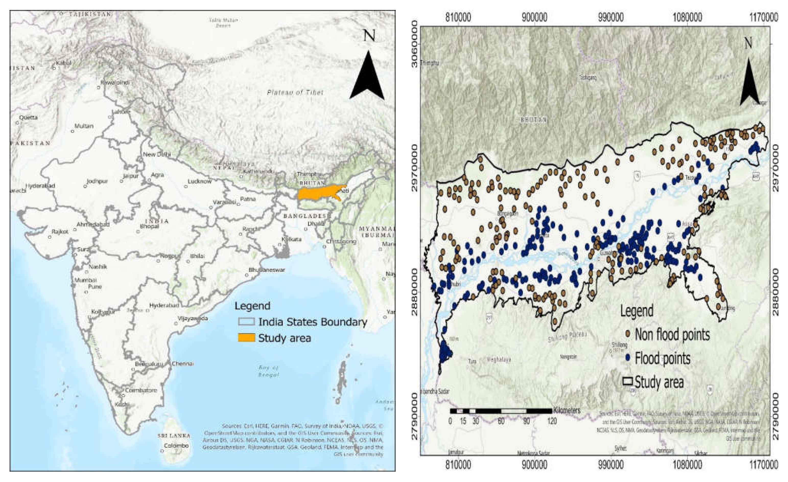
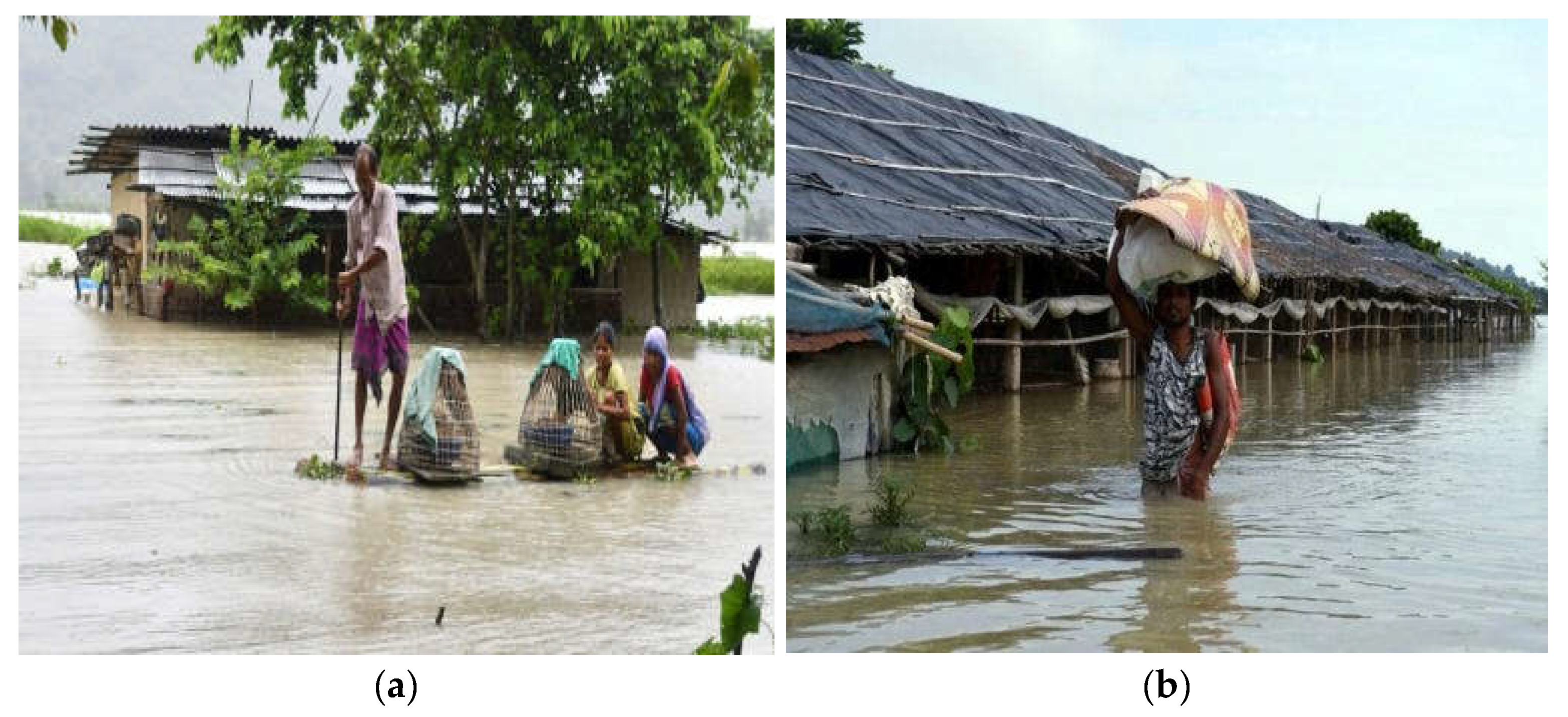
2.1. Study Area

The study area lies in the Assam region, India, extending from 22°19′ to 28°16′ north latitude and 89°42′ to 96°30′ east longitudes (Figure 1). The study area covers around 33,908.14 km2 in the region, with an altitude range of 45–1960 m above mean sea level. As the state of Assam experiences tropical monsoon climates, it receives heavy rainfall (2300 mm annually) and maintains high humidity. Nearly 75% of precipitation occurs during the monsoon spell (July to September) each year. During the winter season, it experiences low humidity and moderate temperatures. The seasonal temperature varies between 8 °C and 32 °C.
Torrential precipitation in the rainy seasons and the rising water levels of the Brahmaputra river and its branches cause floods in different parts of the state every year. The disaster also leads to loss of human life and animals and damage to crops, construction, transportation, communication systems, etc. The devastating floods that hit the state of Assam in 2015 caused a loss of 42 people and affected over 1.6 million households. The disaster also destroyed over 2000 villages and damaged over 440,000 acres of cropland. In July 2016, the flood forced the evacuation of more than 1.7 million people and damaged major roads in the state. Floods in the state of Assam also affect neighboring states such as Nagaland and Manipur. Similarly, in 2018, the floods affected around 0.45 million people and submerged over 11,243 hectares of cropland in four districts of Assam [11]. In 2019, the disaster affected nearly 0.52 million people in 3024 villages. The Assam Disaster Management Authority (ASDMA) reported that, even in the 2020 flood, more than 30,000 households were affected, including half of Kaziranga National Park and Pobitora Wildlife Sanctuary. In addition, around 87,000 hectares of farmland were devastated in the 2020 flood that came along with the COVID-19 pandemic (Figure 2a). During the 2022 flood, more than 6000 households were affected, and more than 60,000 hectares of agricultural land were destroyed across the state (Figure 2b). The frequent flood in the study area demands flood hazard mapping with new technologies.

2.2. Historical Flood Inventory Mapping

Accurate FHZ mapping depends on different flood-causative factors suitable for the study area. Historical flood information is required to validate the flood hazard zones. The annual flood frequency of the study area is as high as 9–10, affecting around 40% of the state. The country has a flood-affected area of around 10%, which makes the region four times more prone to flooding in terms of the national average. The Assam region had major floods in 1954, 1962, 1966, 1972, 1974, 1978, 1983, 1986, 1988, 1996, 1998, 2000, 2004, 2008, 2015, and 2018 (Government of Assam Water Resources) after independence. Historical flood point location data were collected from the flood annual layer of Web Map Service (WMS) maps from 1999 to 2010. The flooding hazard zone developed by the Bhuvan National Remote Sensing Centre (NRSC), India, field photographs, and damage site-based handheld global positioning system (GPS) points of 2020 and 2021 data were also collected for the flood inventory mapping in the study area. In the flood model analysis, the database was assigned a binary composition, with 200 flood points represented as ‘1′ and 200 non-flood points represented as ‘0′ in the study area. For cross-the validation and accuracy of model prediction, the datasets were classified into training and testing groups by 70%:30%.

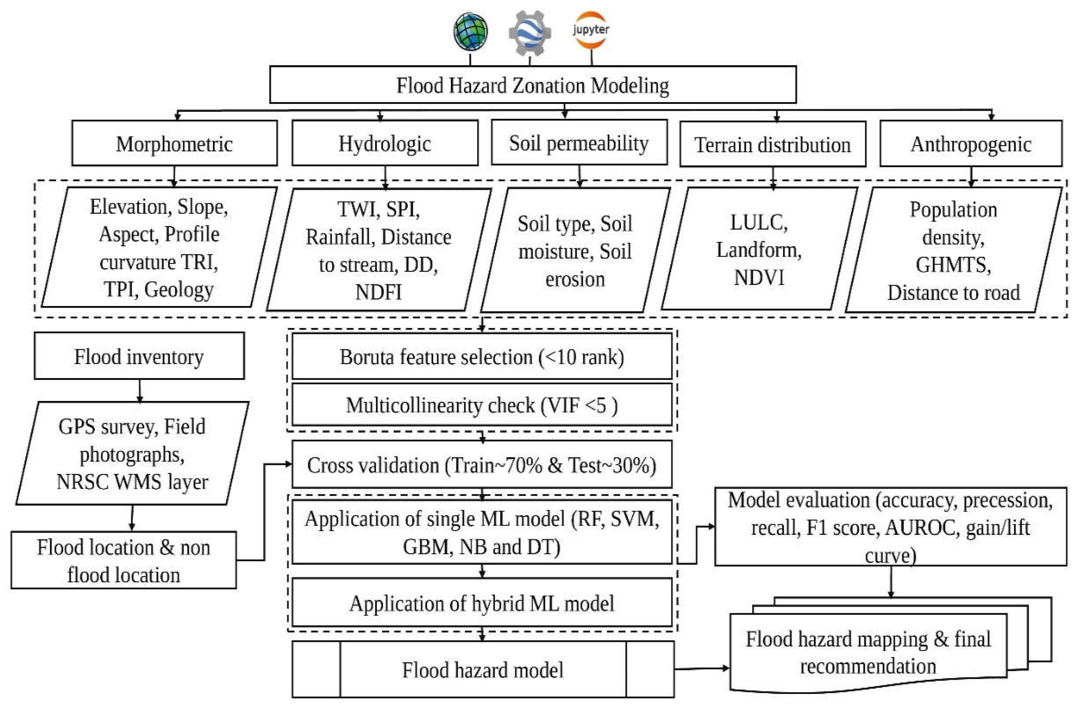
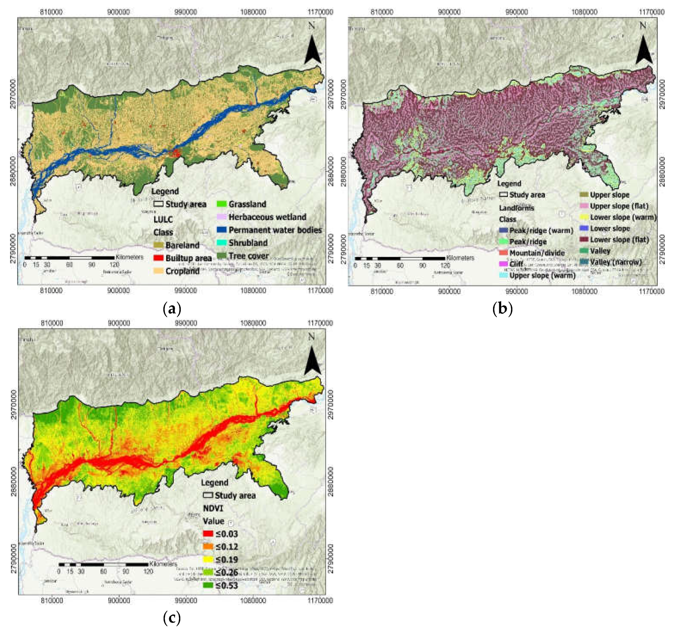
2.3. Flood-Causative Factors

Characteristics of floods vary from location to location based on their geoenvironmental variability. The geographical behaviors of the study area were analyzed by selecting the flood-causative factors (FCFs). A comprehensive literature review and communication with local hydrologists and administrators were carried out to assist in choosing the twenty-two factors, including seven morphometric factors (elevation, aspect, slope, profile curvature, topographic ruggedness index (TRI), topographic position index (TPI), and geology), six hydrological factors (topographic wetness index (TWI), standardized precipitation index (SPI), rainfall, distance to stream, drainage density (DD), and normalized difference flood index (NDFI)), three soil permeability factors (soil type, soil moisture, and soil erosion), three terrain distribution factors (land use/land cover (LULC), landform, and normalized differential vegetation index (NDVI)), and three anthropogenic factors (population density, Global Human Modification of Terrestrial System (GHMTS), and distance to road) for FHZ analysis. All the thematic maps (30 m spatial resolution) were prepared using the data sources for FHZ in the ArcGIS 10.7 (ESRI, Redlands, CA, USA) environment. The details of FCFs used in this study, including all the preprocessing steps and methodological framework for FHZ, were formulated in a flowchart for the research work (Table 1 and Figure 3).

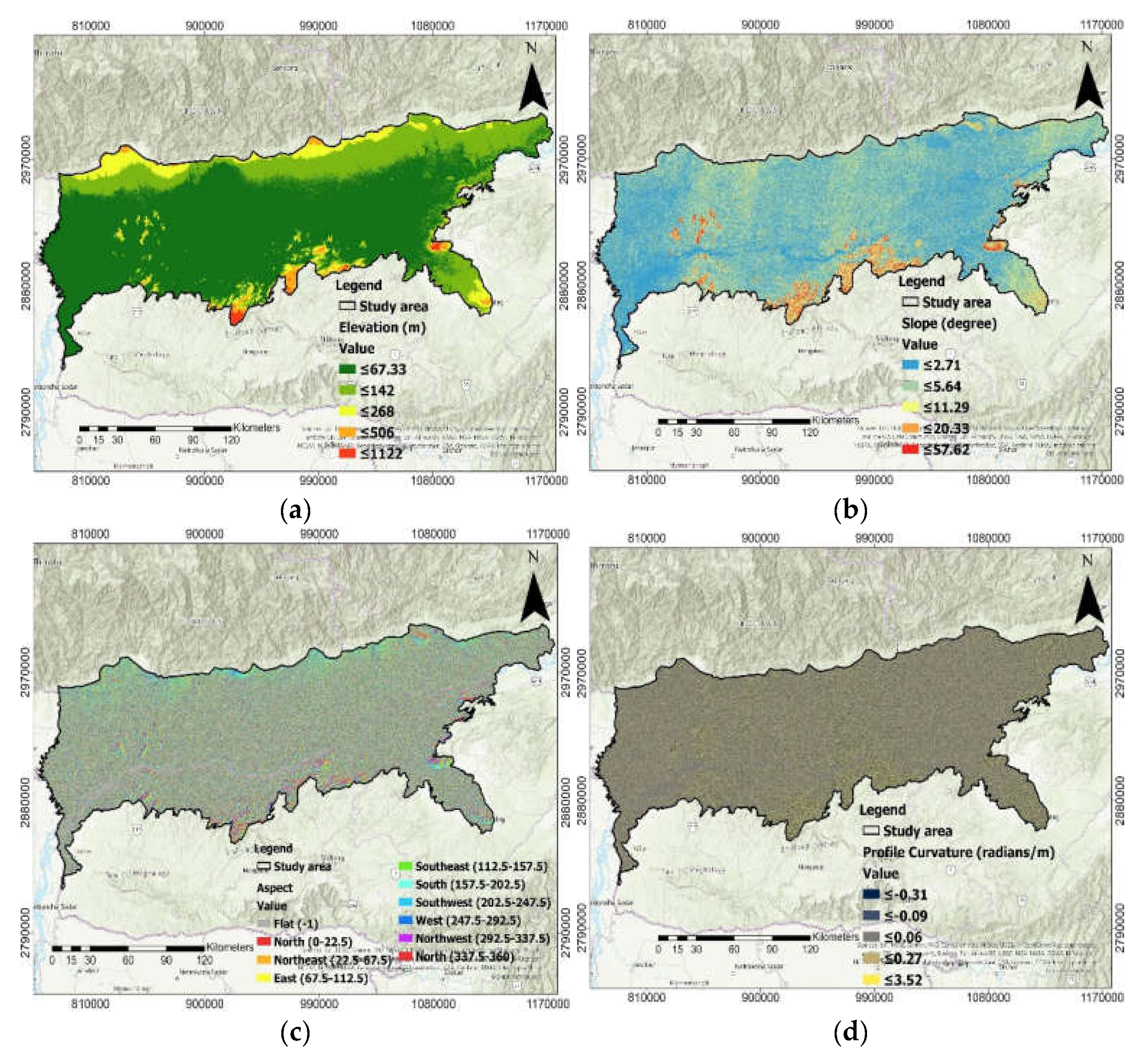
2.4. Morphometric Factors

The seven depicted flood conditioning factors, grouped under morphometric criteria, were derived from the Advanced Spaceborne Thermal Emission and Reflection Radiometer (ASTER) (GDEM) data of 30 m resolution. Elevation is the main criterion for predicting areas of flood occurrence. Flood occurrences are high in low-elevation zones in comparison to high-elevation areas [33]. Slope also monitors subsurface runoff amount, sedimentation, infiltration rate, and flow accumulation level. Flood direction and duration are also delineated by aspect and slope gradient factors. Degree of slope and aspect map were extracted through the Google Earth Engine code editor. Profile curvature represents the variation of convexity and concavity of relief features [34]. Topographic position index (TPI), a component of terrain surface plane, represents deviation from the central cell to the surrounding cell. Topographic ruggedness index (TRI), which represents the region’s undulating characteristics, has an inverse relationship with flood susceptibility level [35]. TPI and TRI were derived from DEM using ArcGIS software v10.7 (Equations (1) and (2)).
T P I = E c e l l E s u r r o u n d i n g
T R I = A b s m a x 2 m i n 2
where E c e l l represents the elevation of the pixel;
E s u r r o u n d i n g represents the average elevation of the neighboring cell;
max and min represent maximum and minimum elevations, respectively.
Five geological units (mesozoic and paleozoic intrusive metamorphic rocks, undivided precambrian rocks, paleogene sedimentary rocks, undivided paleozoic rocks, and quaternary sediments) were identified. Quaternary sedimentary geological units occupy a maximum area of 70% in the study zone.
The elevation of the study region varies from 67 to 1122 m (Figure 4). The profile curvature in the study area ranges from −0.31 to 3.52 (Figure 4d). TPI and TRI were categorized into five classes using the natural break Jenks method. TPI and TRI ranged from −2.41 to 24.12 and 24.93 to 397.38 within the region of study in the categorical geological map extracted from the U.S. Geological Survey World Energy Project, 2000 (Figure 4e,f).

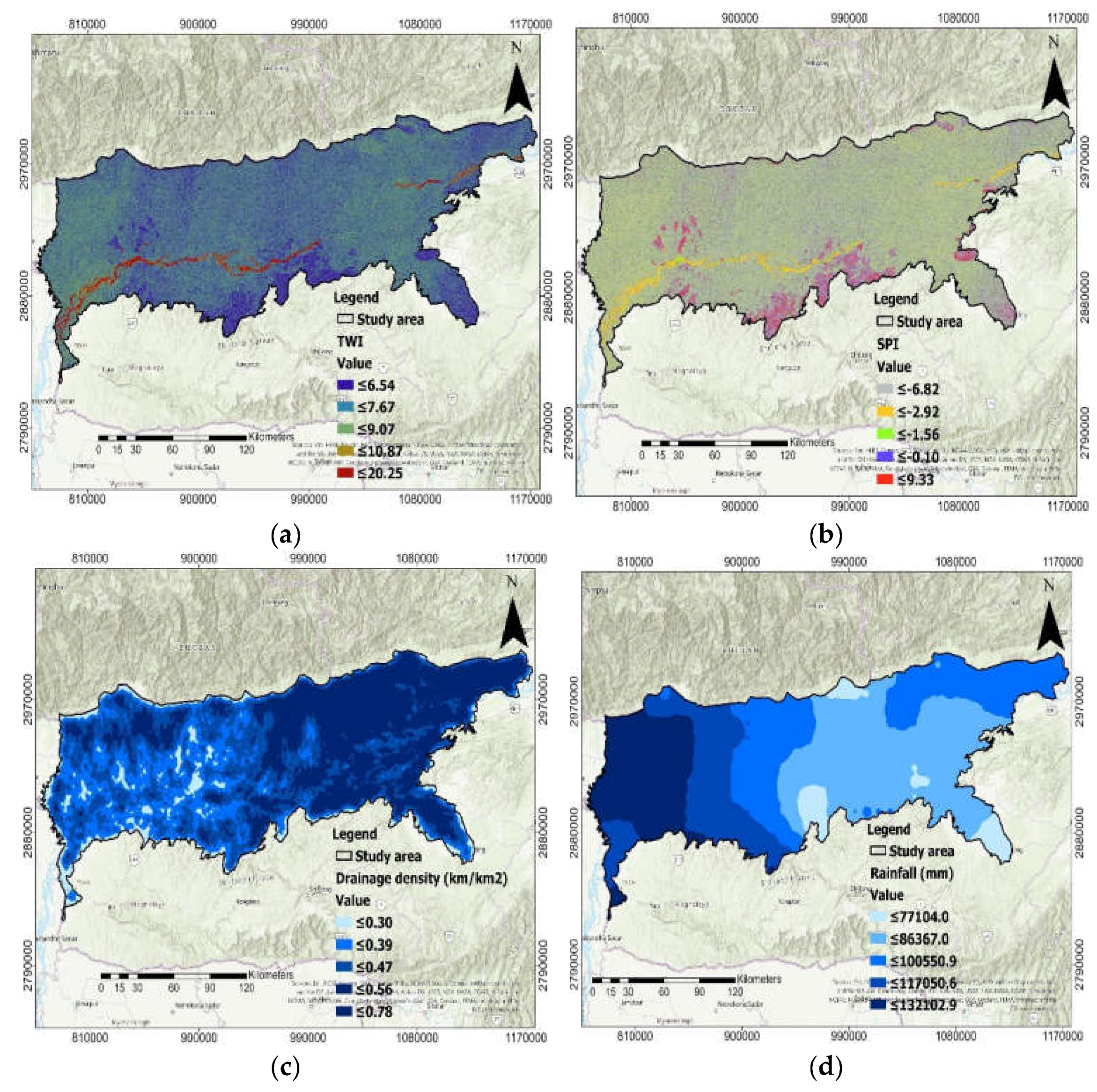
2.5. Hydrologic Factors

Topographic wetness index (TWI) and standardized precipitation index (SPI) factors were estimated from digital elevation model (DEM) data using the ArcGIS tool (Equations (3) and (4)). Flood flow intensity is greatly controlled by the gravitational effect, which accounts for TWI distribution. TWI is a widely used geohydrological process influencing basin moisture level, soil depth, water table, and saturated zone management [36]. SPI explains the erosive efficiency of flowing water within a particular point, reciprocal to flood occurrences [37]. The drainage density (DD) map was computed through the line density tool in the ArcGIS software environment with the help of the HydroSHEDS free-flowing river network tool (Equation (5)).
Duration and intensity of rainfall generally determine flood acceleration rate after a rainfall event. Mean annual rainfall data for the years 2000–2020 were extracted from Climate Hazards Group InfraRed Precipitation with Station data (CHIRPS v2.0, developed by USGS Earth Resources Observation and Science (EROS) Center, Santa Barbara, CA, USA) in ArcGIS 10.7 software environment through the inbuilt inverse distance weighting (IDW) tool and were used for preparing the rainfall distribution map. Annual rainfall in the study region varied between 771 mm and 1321 mm (Figure 5d). Drainage density monitors runoff rate, infiltration rate, and permeability, which employs the supplementary likelihoods of a flood event. Flood occurrence was directly proportional to the distance of the location from the rivers [38]. The Euclidean distance tool was used for producing the distance stream map in the ArcGIS environment. The normalized difference flood index (NDFI) was computed using the RED and SWIR2 bands of Sentinel 2B MSI data in the GEE platform [39] (Equation (6)).
T W I = I n A i / tan β
S P I = A i × tan β
where A i : basin area;
β : degree of gradient slope.
D D = i = 1 n Z i A i
where: i = 1 n   z i sum of stream length (Z);
A i : total basin area;
‘n’: number of streams within the area.
N D F I = R E D S W I R 2 R E D + S W I R 2
where NDFI: normalized difference flood index; RED and SWIR2: reflectance values for the Red and SWIR2 band spectrum, respectively.
TWI and SPI values ranged from 6.54 to 20.25 and −6.82 to 9.33 (Figure 5a,b). Drainage density was classified into five zones, namely, ≤0.30 km/km2, ≤0.39 km/km2, ≤0.47 km/km2, ≤0.56 km/km2, and ≤0.78 km/km2 (Figure 4c). Distance to rivers was categorized into five classes (≤327 m, ≤695 m, ≤1076 m, ≤1567 m, and ≤3475 m). The range of the NDFI value was between 0.16 and 0.99.

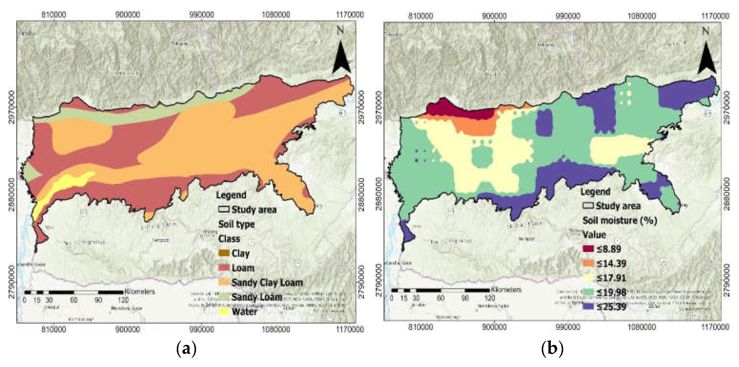
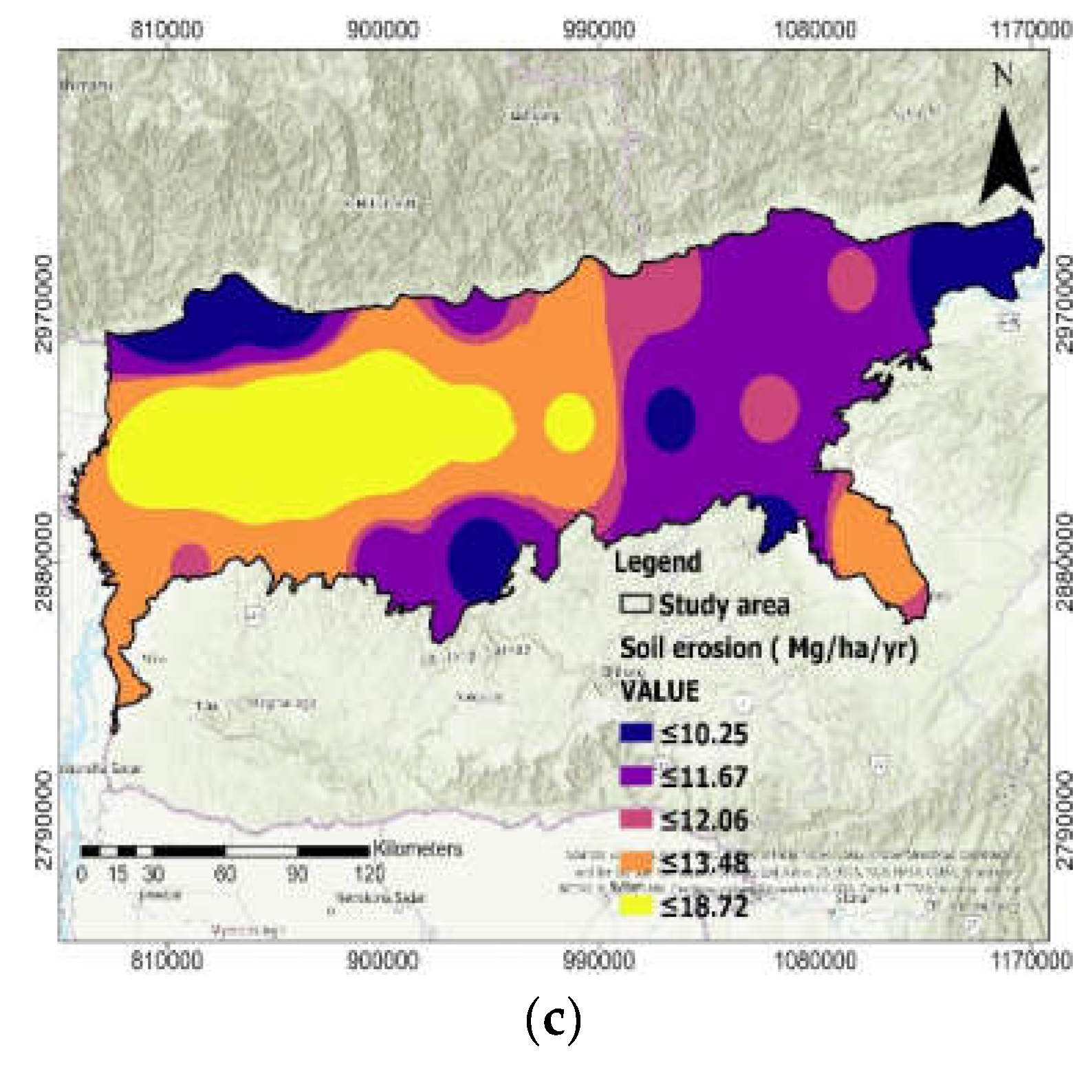
2.6. Soil Permeability Factors

Soil type, a predisposing factor of floods, determines the soil permeability rate, soil percolation rate, and rate of runoff. The soil map of the study site was extracted from the Harmonized World Soil Database v1.2 portal. The soil moisture active and passive (SMAP) satellite-derived L-band was used for developing the soil moisture distribution map through the GEE platform. Soil erosion could also trigger flood events due to their sediment load [40]. The soil erosion map was developed from the Global Land Degradation as Debts database.
Four soil types were defined in ascending order of their area coverage in percentages, such as clay (0.06%), sandy loam (8.68%), loam (39.02%), and sandy clay loam (49.88%) (Figure 6a). Five soil moisture zones were demarcated for the study area (Figure 5b). Soil erosion maps were developed from the Global Land Degradation as Debts of the European Soil Data Centre (Figure 6c). The soil erosion rate ranged from 10.25 to 18.72 Mg/ha/y. The central region of the study area received very high soil erosion incidents in the range of ≤18.72 Mg/ha/y (Figure 6c).

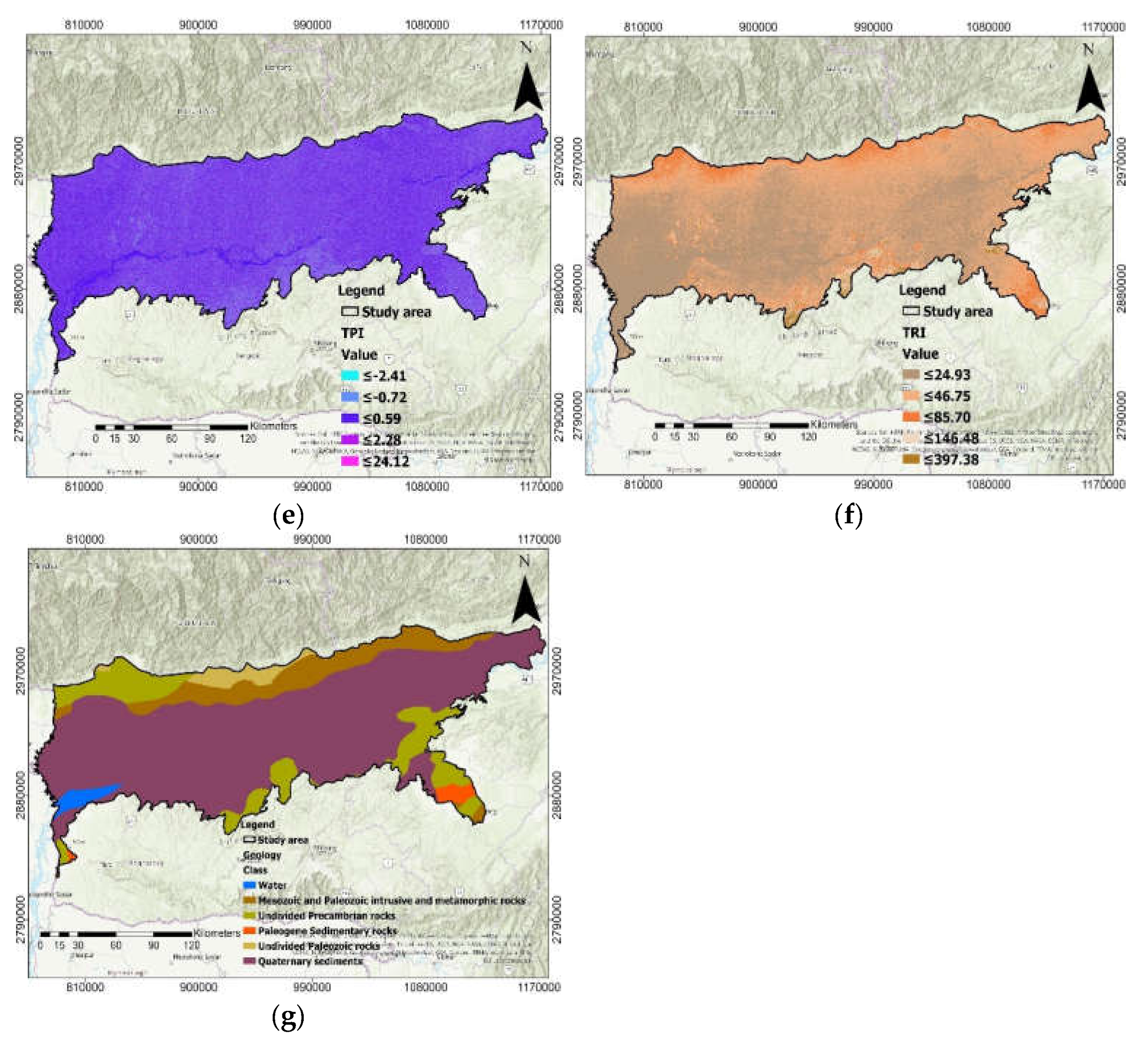
2.7. Terrain Distribution Factors

Land use/land cover (LULC) pattern directly impacts the occurrence of a flash flood. Land area covered with vegetation is less prone to flooding compared to barren land [41]. The LULC map of 2020 was obtained from the European Space Agency (ESA/WorldCover datasets). Global Advanced Land Observing Satellite (ALOS) landform classes are very sensitive to the quantification of land cover zones, as they are ecologically relevant to the physiographic process [42]. The landform layers were obtained from ALOS Polarimetric phased array L-band synthetic aperture radar (PALSAR) data. Twelve landform classes were utilized for FHZ, i.e., peak/ridge (warm), peak/ridge, mountain/divider, cliff, upper slope (warm), upper slope, upper slope (flat), lower slope (warm), and lower slope. NDVI is a good indicator of vegetation coverage, largely inducing soil moisture, evapotranspiration, infiltration, sediment transportation, and runoff. High NDVI minimizes flood events [28] and vice versa. The NDVI layer was prepared from the Sentinel 2B MSI image of 2021 using the NDVI estimation equation (Equation (7)).
N D V I = N I R R E D N I R + R E D
where NDVI: normalized differential vegetation indices;
NIR and RED: reflectance indices for NIR and Red band, respectively.
Eight LU/LC classes were distinguished for the study region. Cropland demarcated the maximum area (47.49%), followed by tree cover (35.51%), permanent water bodies (8.56%), barren land (5.21%), grassland (1.65%), built-up (1.18%), shrubland (0.20%), and herbaceous wetland (0.20%) (Figure 7a). The annual NDVI layer was classified into five levels, and the levels of ≤0.19 occupied the maximum (62.03%) area, followed by the level of ≤0.12 (21.38%), ≤0.26 (14.26%), ≤0.03 (2.03%), and 0.53 (0.30%) (Figure 7c).

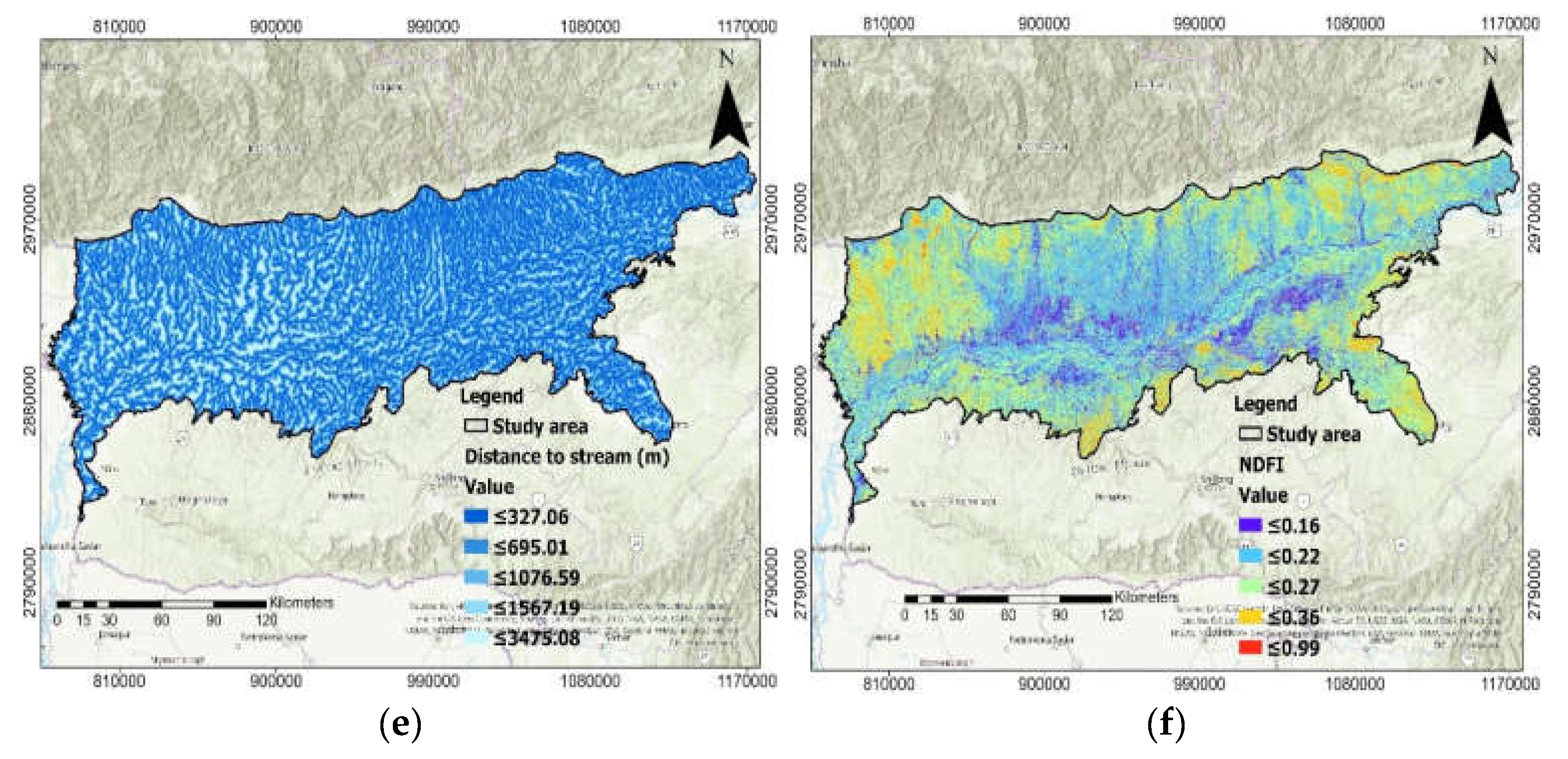
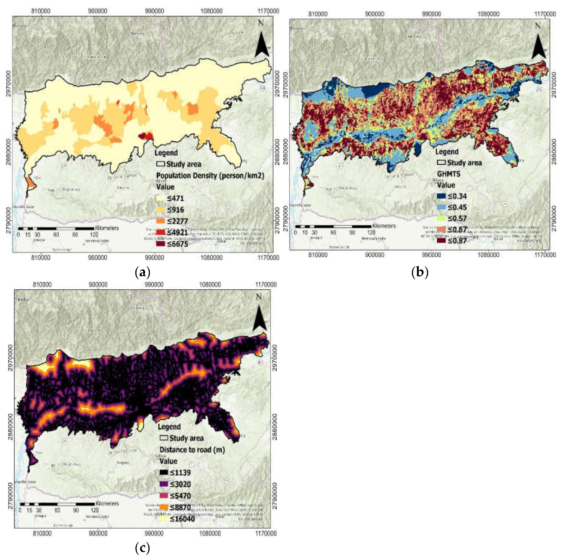
2.8. Anthropogenic Inferences Factors

Population density (PD), one of the major anthropogenic factors affecting all resources, monitors the recharge or discharge of water, infiltration rate, and water flow. The PD map was obtained from the Landsat v1-based GPWv4.11 database through the GEE platform. The Global Human Modification of Terrestrial System (GHMTS) implies different human modification stress that could impact the degree of flood risk [43]. The GHMTS layer was produced from the NASA Socioeconomic Data and Applications Centre database. The distance to the road factor was computed through the Euclidean distance tool in ArcGIS 10.7 software.
This current study has identified five classes of person/km2 level e.g., ≤471, ≤916, ≤2277, ≤4921, and ≤6675 in person/km2 (Figure 8a) for population density analysis. The range of the GHMTS layer was demarcated between 0.34 and 0.87 (Figure 8b). As we know, the nearby roads are highly prone to flood occurrences with their impervious surface and water blockage [12], and distance to road has some impact on the frequency of floods. Distance to road maps is also classified into five categories, namely, ≤1139 m, ≤3020 m, ≤5470 m, ≤8870 m, and ≤16,040 m (Figure 8c).

2.9. Boruta Feature Ranking and Multicollinearity Check

The comparative importance of the flood-influencing factors was visualized before the model’s validation. This step can help in determining the model’s ability to improve prediction accuracy to cope with flood hazard zoning. The efficiency of each factor was measured using the statistical properties of its correlation with flooding and classification status. The Boruta feature ranking technique was used to identify the most significant factors for the forecast of FHZ [14]. Here, the randomness was given to the data set by creating shuffled copies of all features (shadow data set). Then, the iteration process checked whether a real feature has a higher importance than the best of its shadow features. The iteration continued until all the features were either confirmed or rejected. The Boruta feature selection helped in achieving the optimum accuracy and reducing the model overfitting problems. The random forest method identified the relative importance of the flood susceptibility factor in the Boruta feature selection. The variance inflation factor (VIF) technique was used for checking the multicollinearity problem of each FCF. The model can give sound performance when the VIF is less than 5, indicating the absence of collinearity in the factors [44]. The VIF was calculated as follows (Equations (8) and (9)).
T o l e r a n c e = R j 2
where R J 2 : coefficient of determination of regression of explanatory J on all the other explanatories
V I F = 1   T o l e r a n c e  
where VIF: variance inflation factor; Tolerance: tolerance level.

2.10. Machine Learning Model

2.10.1. Random Forest

The random forest (RF) model is an ensemble tree-based machine learning model coined by Breiman [45]. The goal of an ensemble learning technique is to combine the training of various decision trees into a single prediction. RF can also be used to estimate the accuracy of various decision tree classifiers on different subsample points (bootstrapping) when building trees (ntree). It uses simple averaging to improve its accuracy and control overfitting while maintaining the subsample size. In the RF technique, if the bootstrap criterion is True, then the whole dataset is used to build the tree.

2.10.2. Support Vector Machine

The support vector machine is very efficient in high-dimensional spaces. It can be very useful where the number of samples is greater than the number of training points. It also uses a subset of the decision function (support vectors) and regularizes factors to perform memory-efficient calculations. There are many types of kernels, e.g., ‘linear’, ‘radial basis (rbf)’, ‘sigmoid’, ‘poly’, and ‘precomputed’, that can be specified for the decision attributes of the model. Several studies have reported that the ‘rbf’ function outperforms others for flood risk modeling [46].

2.10.3. Gradient Boosting Model

The powerful ensemble gradient boosting algorithm (GBM) is used for performing various calculations associated with the regression and classification of tabular data. The GB model is an additive framework that permits the execution of differentiable loss functions in a forward-looking manner and reduces the error gradient. In each stage, a regression tree is fitted to the negative classifier of the calculated loss function. The main parameters that the GBM algorithm considers for FHZ when it comes to performing various hyperparameters are learning rate, maximum tree depth, minimum tree weight, regularization alpha, and lambda [47].

2.10.4. Naïve Bayes

Naïve Bayes methods are based on the Bayes theorem, which states that every feature of a class variable has conditional independence of probability [48]. The ability to decouple the class conditional feature agrees with Bayes methods to accomplish fast and precise classification and learning tasks. This eliminates the need for further investigation related to dimensionality patterns.

2.10.5. Decision Tree

A decision tree (DT) is a type of supervised learning method that can model simple decision rules found in the data features. DT takes place in a tree structure such as decision nodes and end nodes with categorical, binary, and continuous variables [49]. It works as a white box model for feature selection. Gini index, information gain, and chi-square methods were used for making a decision tree.

2.10.6. Hybrid Modeling

All four above-mentioned models used the stacking method to develop the hybrid machine learning model. Model evaluation and performance analysis were used through VotingClassifier in the scikit-learn library through the Anaconda Jupyter notebook v6.1.4. Currently, hybrid machine learning is very popular for FHZ [16,24,50]. All ML classifier analyses use the sklearn OneHotEncoder, GridSearchCV, and the pipeline approach in Python for continuous and categorical data to generate FHZ. All the ML models performed well through the best tuning optimization incorporated into twenty-two flood-causative factors (Table 2).

2.11. Model Validation and Performance Evaluation

As statistical measures, the precision, recall, F1 score, area under the curve (AUC), and model accuracy were applied to assess the performances of the ML models (Equations (10)–(13)). Model accuracy can specify the validation result for witnessed flood pixels and nonflood pixels. AUROC analysis represents the true-positive rate (specificity value) and false-positive rate (sensitivity value) of the probability of floods and nonflood pixel ratios, which are correctly classified. AUC performance considers model reliability and exactness. An AUC value range between 0 and 1 was used in Equation (14). A higher AUC value influenced the better acceptability of the model optimization [22].
p r e c i s i o n = T P T P + F P
r e c a l l = T P T P + F N  
F 1 = 2 × p r e c i s i o n × r e c a l l p r e c i s i o n + r e c a l l
Accuracy   = T P + T N T P + F P + T N + F N
where true positive (TP) and true negative (TN) are correctly predicted pixel numbers;
False positive (FP) and false negative (FN) are falsely predicted pixel numbers;
P: total number of floods;
N: total number of nonfloods denoted by N.
The cumulative gain curve is used for the model benefits and effectiveness of flood and nonflood pixels. The cumulative gain curve shows the performance of the mentioned model when it estimates new targets that can be reached based on a given population. It shows the percentage of individuals that our model can realistically reach with the highest probability of being successful. The cumulative gain curve is a graphical representation between the gain on the vertical axis and the decile (percentage of the sample) on the horizontal axis. The lift curve is a ratio of the number of positives that the model can influence the probable number of negative observations that it considers zero within a random space. The lift curve demonstrates the association between the positive and negative records of deciles. The larger the area between the gain/lift and baseline, the better the model works (Equations (14) and (15)).
Gain   =   Cumulative   number   of   positive   observations   upto   decile   k     Total   number   of   positive   observations   in   the   sample  
Lift   =   Cumulative   number   of   positive   observations   up   to   decile   k   using   ML   model     Cumulative   number   of   positive   observations   up   to   decile   k   using   a   random   model  
where Gain: gain in terms of positive observations;
Lift: association between positive and negative records.

3. Results

3.1. Multicollinearity Test and Boruta Feature Ranking

Multicollinearity testing and Boruta feature ranking of the twenty-two flood monitoring factors were carried out (Table 3). The VIF ranged between 1.07 and 3.28, and the uppermost and lowermost values of VIF were assigned with NDFI and TWI. As all the values of VIF were within the limit (<5.0), there was no multicollinearity problem among the flood-influencing factors. The result of the Boruta method found that fourteen factors were the most important (Rank 1) for the current study, namely, elevation, landform, soil moisture, slope, TRI, LULC, NDVI, NDFI, distance to stream, rainfall, population density, GHMTS, distance to road, and geology (Figure 4a). In contrast, SPI, TWI, and soil erosion had a moderate (Rank 2) influence on flood events, whereas drainage density, profile curvature, TPI, soil type, and aspect had the least importance (Ranks 3, 4, 5, 6, and 7) for FHZ [19].

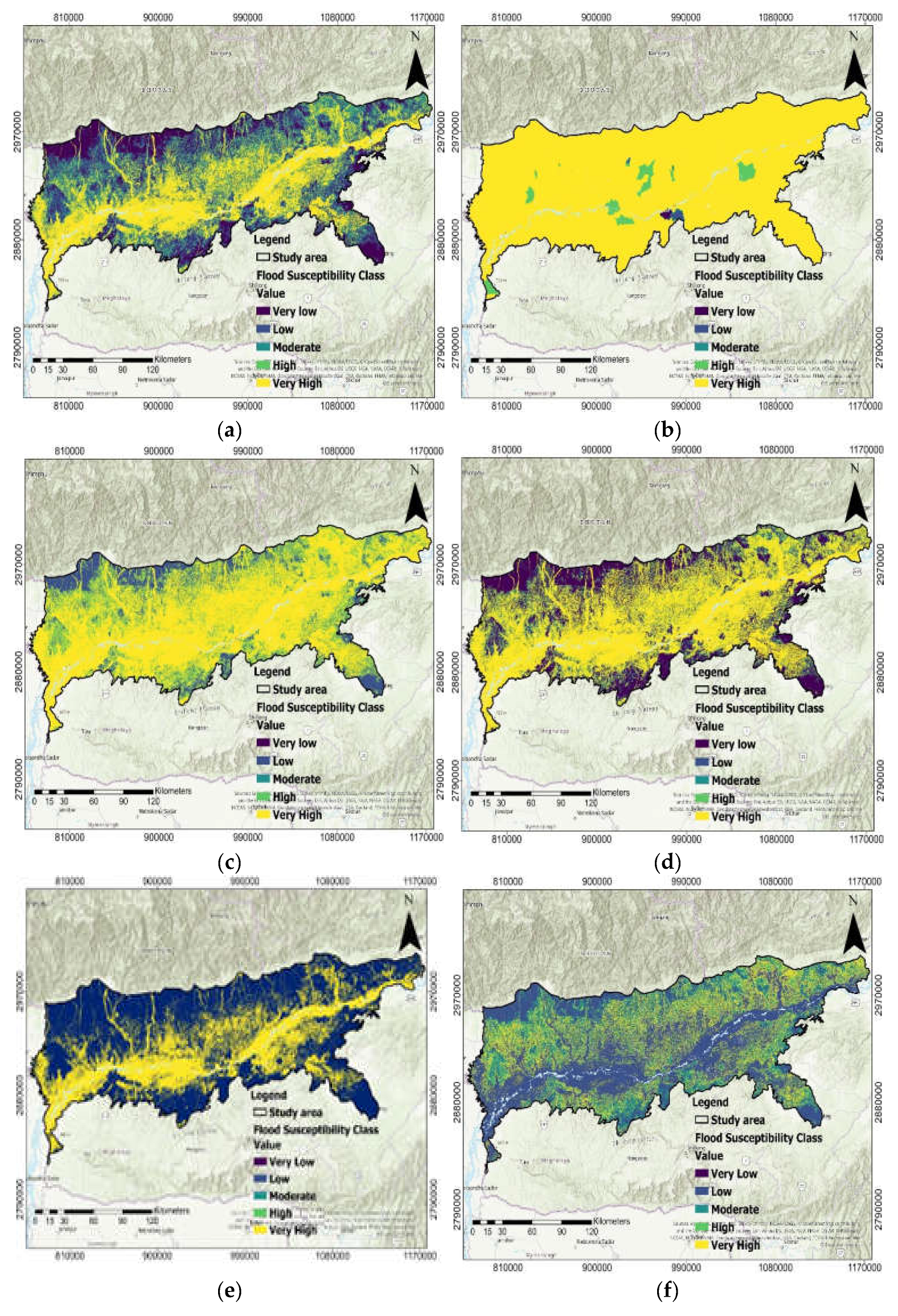
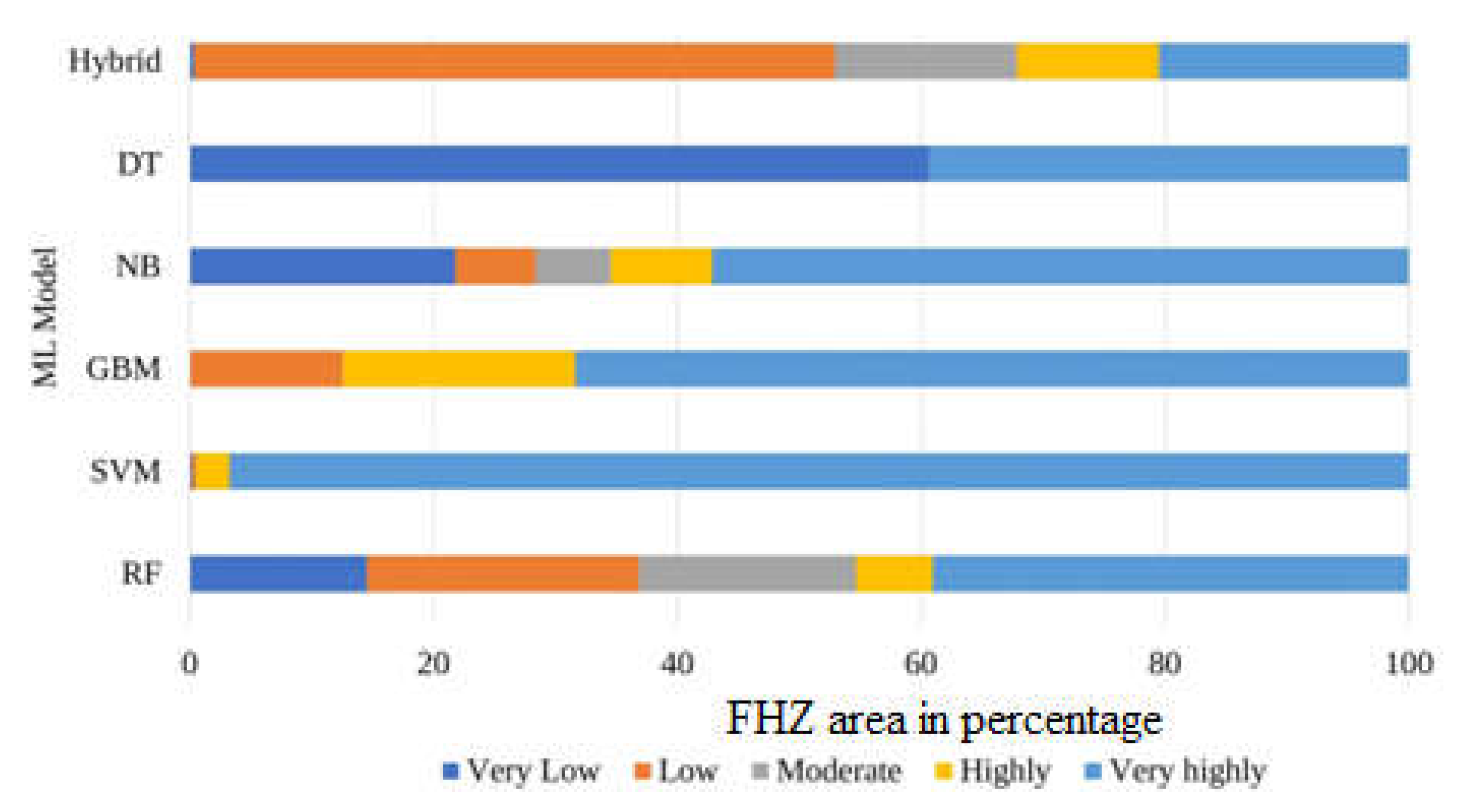
3.2. Flood Hazard Zoning

Spatial analysis of FHZ was created using five ML models of RF, SVM, GBM, NB, and DT and one hybrid model in the Assam region of India. All of these ML models’ output maps were reclassified into five flood hazard zones (i.e., very low, low, moderate, high, and very high) using the well-defined natural Jenks method through the ArcGIS tool (Figure 8). Based on the RF model, 39.07% of the study region was classified as a very high flood hazard zone, whereas 14.52% and 22.32% of the region were very low and low flood-prone areas, respectively (Figure 8a). In the SVM model, the aerial coverage of very high and high flood-prone areas was 96.74% and 2.73%, respectively. In the instance of the GBM model, the arranged FHZ map revealed in terms of aerial coverage for the five zones was very high, 23,180.38 (68.36%); high, 6471.47 (19.08%); moderate, 0.23 (0.001%); low, 4252.89 (12.54%); and very low, 3.18 (0.009%) km2. In the NB model, the areal coverage of very low, low, moderate, high, and very high flood-prone zones was 7387.47 (21.79%), 2233.54 (6.59%), 2092.41 (6.17%) 2815.44 (8.30%), and 19,379.27 (57.15%) km2, respectively (Figure 8). According to the DT model, 39.35% and 60.65% of the study area fall into the very high and very low flood hazard zones (Figure 9). Lastly, the outcomes produced in the hybrid ML proposed that 6952.78 km2 (20.50%) of the study region was in very high flood hazard zones, whereas 5076.56 (14.97%) km2 had a moderate chance of flooding (Figure 9f). According to this model, 52.55% of the study region was under a low flood-prone area (Figure 10), which was represented as the optimum area among all the models. The general rule of thumb as revealed during the research was that the area near the courses of the river was very high flood-prone, and the remote to upper part courses was very low flood-prone.
This region is more prone to floods because of the presence of the Brahmaputra river, with high sediment load during monsoon periods and high runoff coming down from the uphill to the lower confluence river, causing a flash flood event. Accordingly, the blend of morphometric, hydrologic, soil permeability, terrain distribution, and anthropogenic inferences is the main monitoring factor for a higher inclination of overflowing along the courses of the riverbank of the study area.

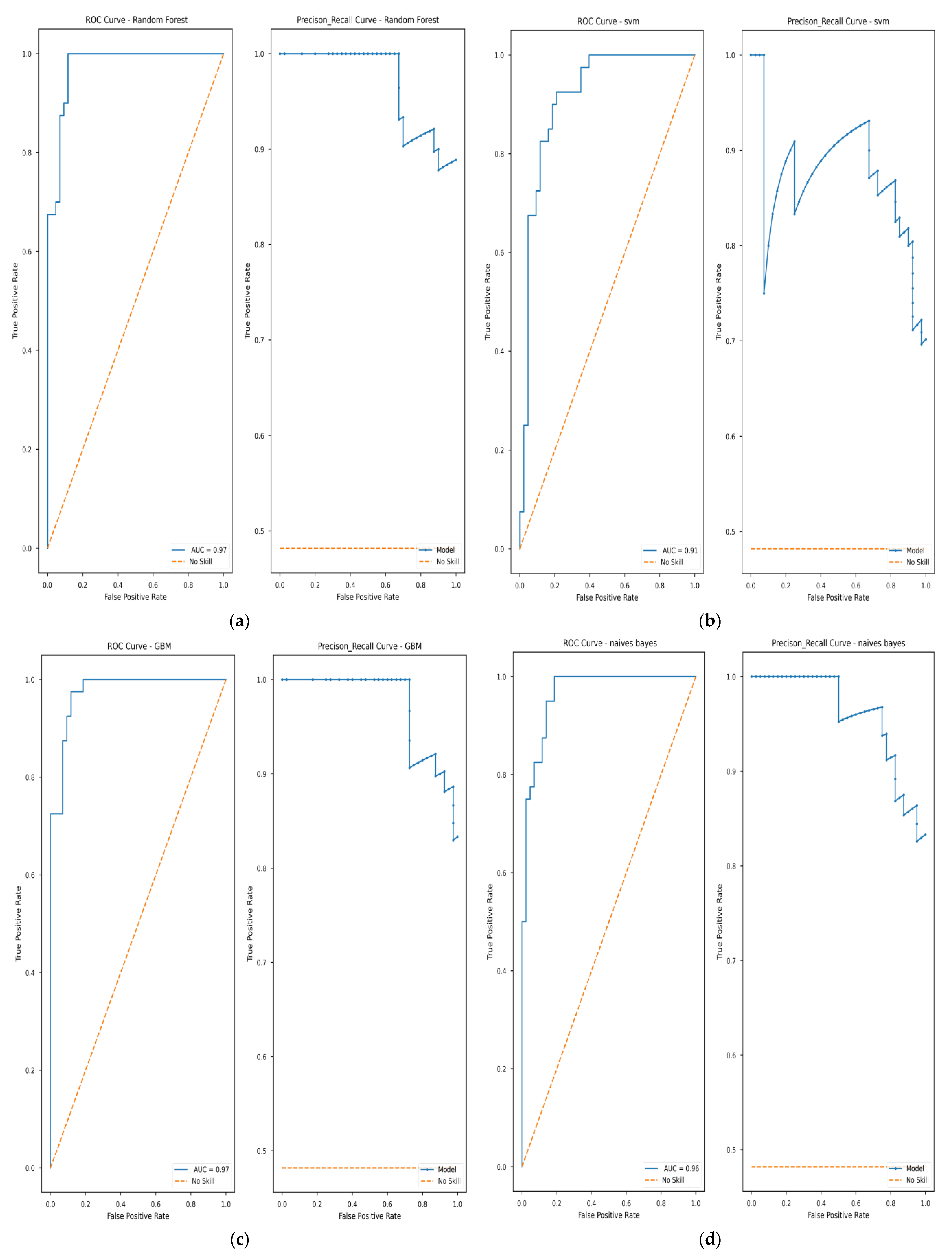
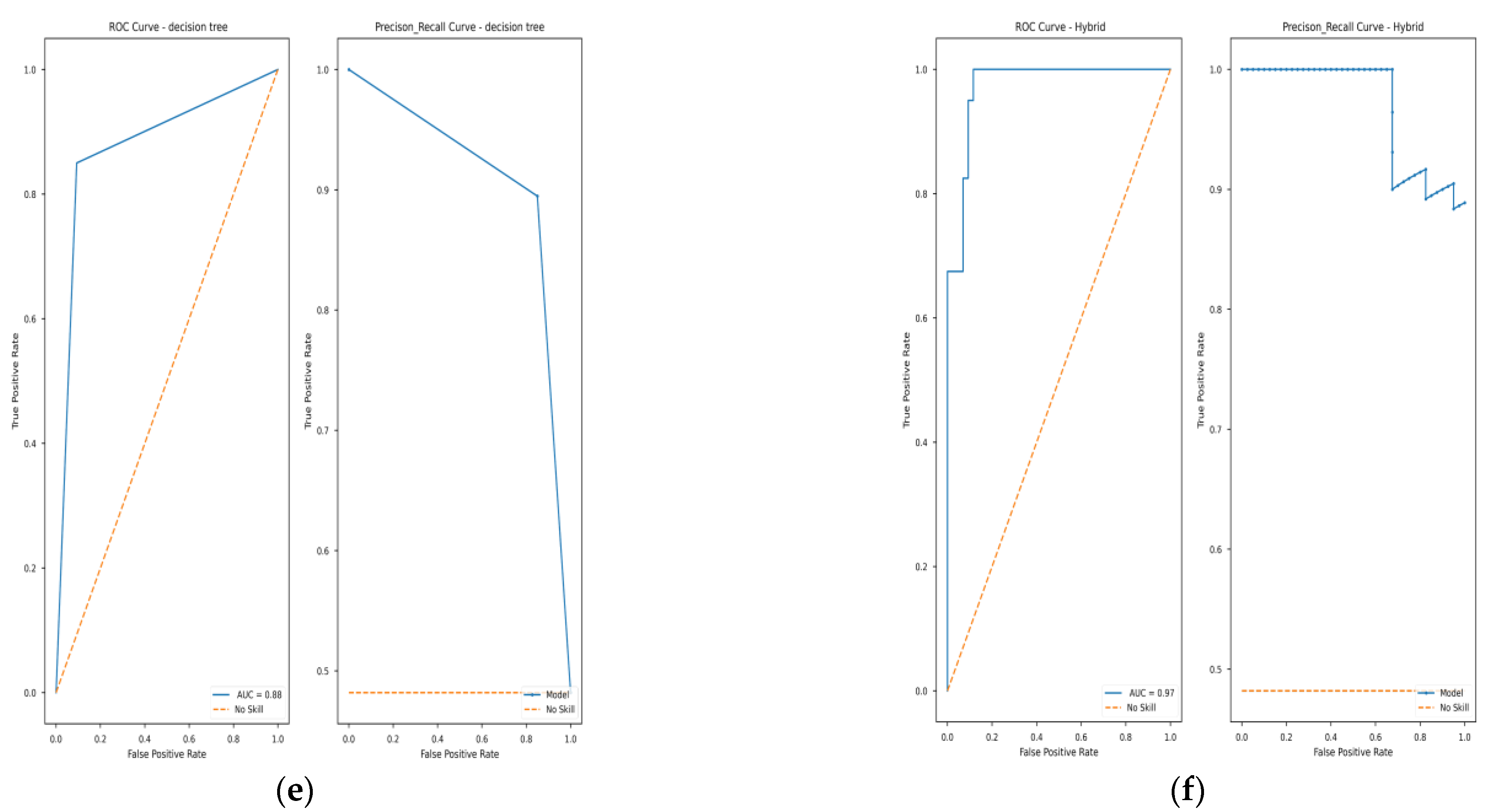
3.3. Validation of ML Models

The single validation method is inadequate for the verification of the flood susceptible zones with the uncertainty of the data variability. Therefore, in this study, we used different ML metrics to verify the outcome, such as accuracy, precision, recall, F1 score, and AUROC.

3.3.1. AUROC Evaluation

The model accuracy of the testing sample and the NB model was very well fitted compared to the others. The AUROC value was higher than 95% for the hybrid, RF, NB, and GBM models, followed by SVM (91%) and DT (88%) (Figure 11). The precision values of the RF and hybrid models were 0.94 and 0.95, respectively (Table 4). Similarly, the recall values of the SVM and hybrid models were 0.97 and 0.92, respectively (Figure 11). The F1 scores of the GBM and hybrid models were 0.91 and 0.93, respectively. This research found that the hybrid model and others, namely, the RF, GBM, and NB models, performed well with their higher metrics value for FHZ analysis.

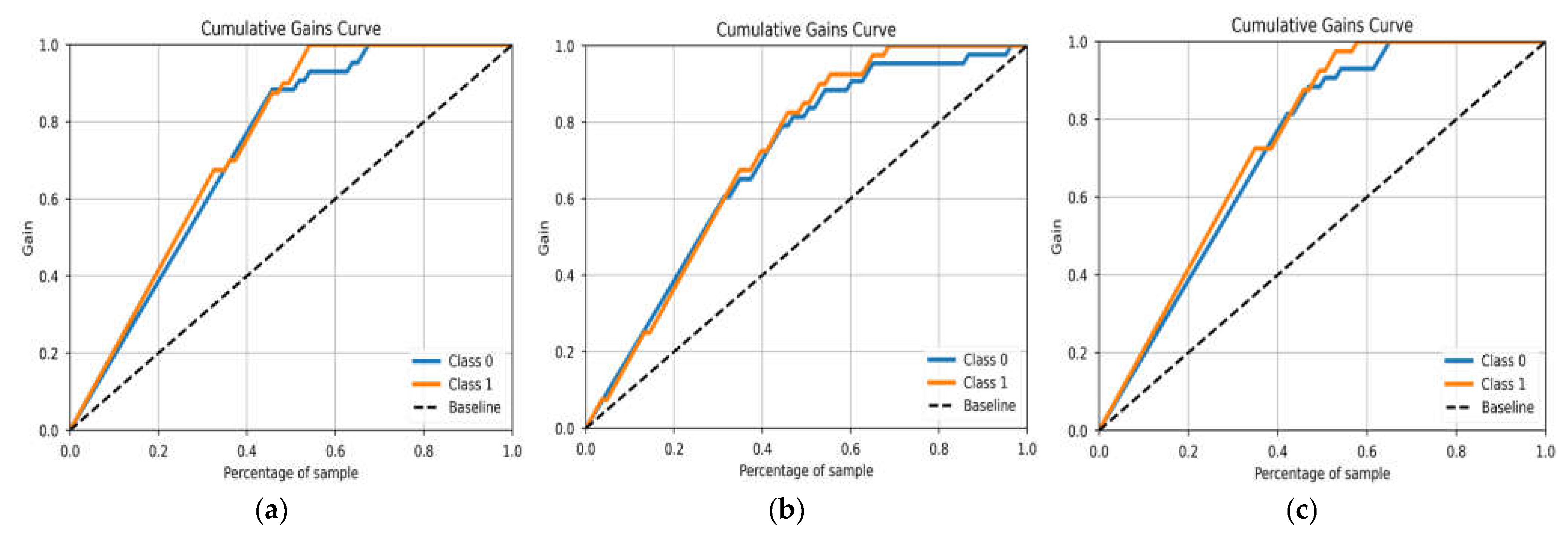
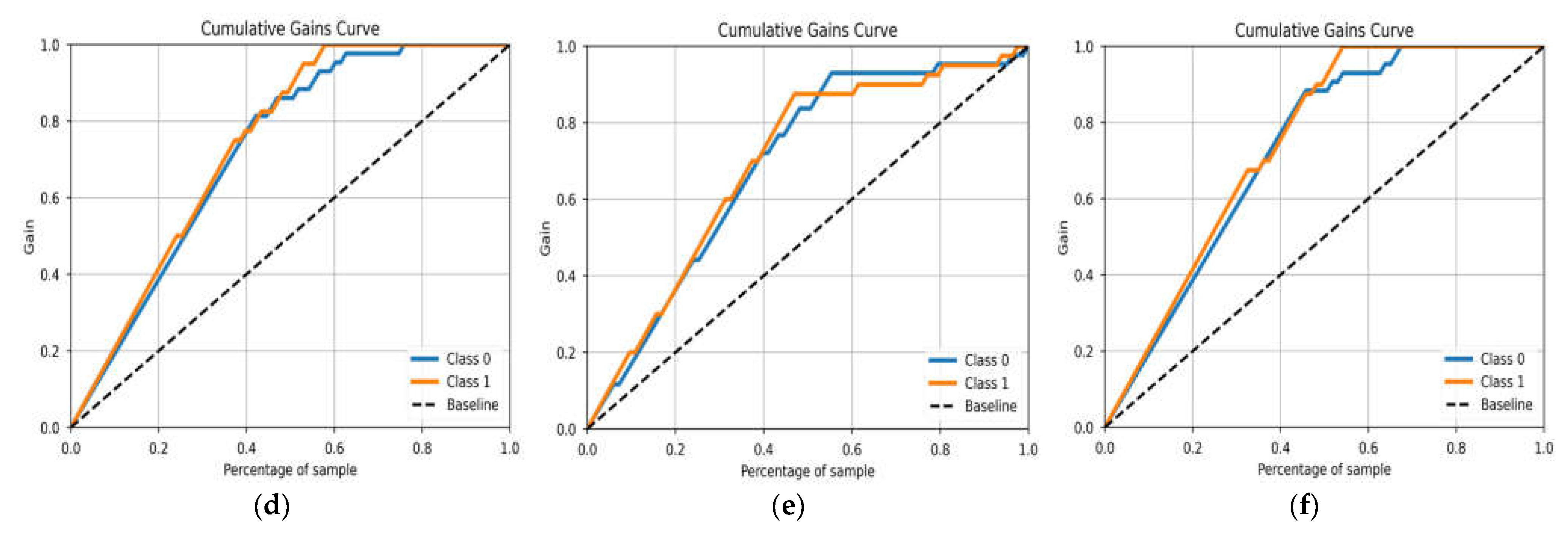
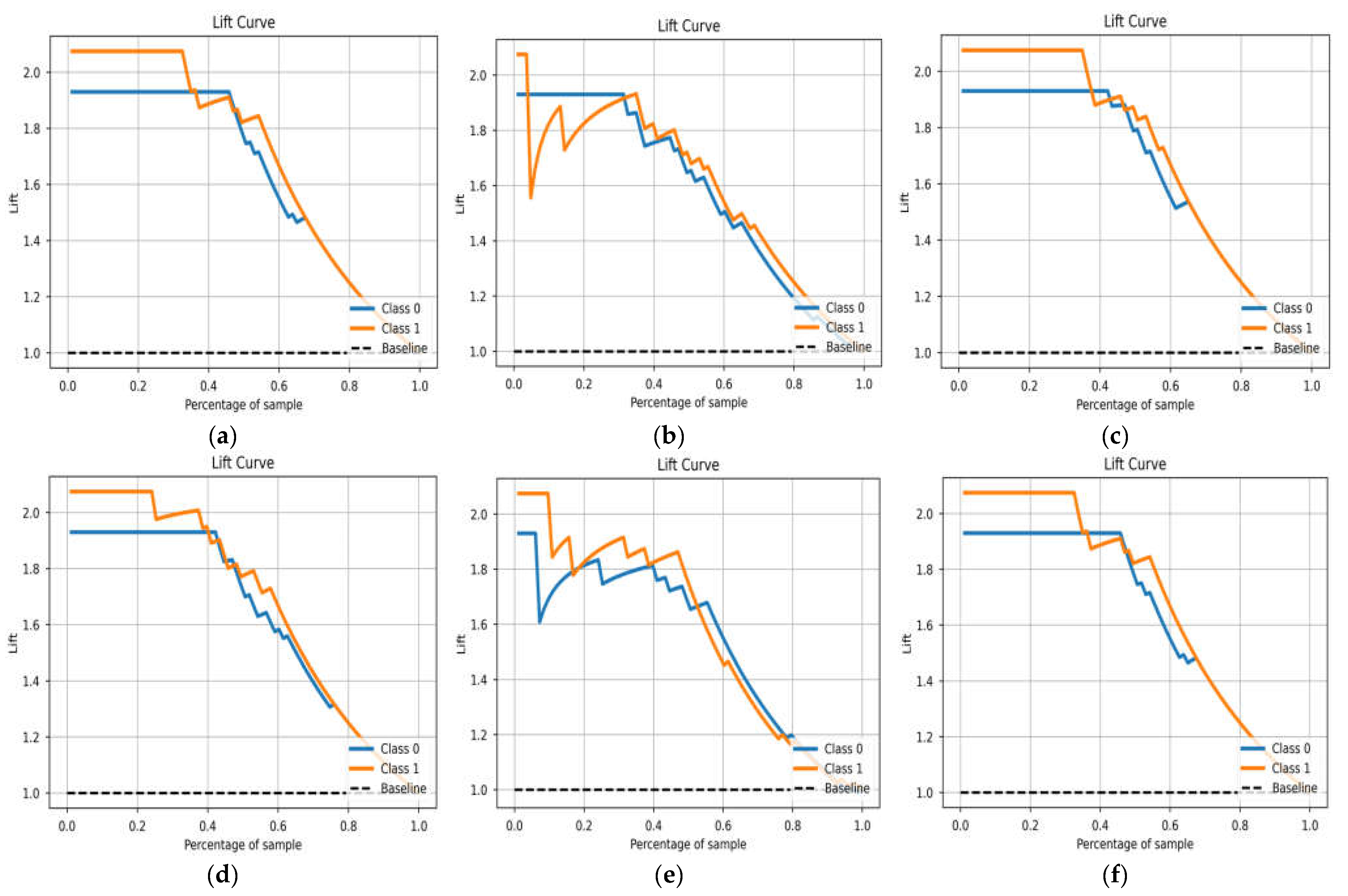
3.3.2. Cumulative Gain and Lift Curve Evaluation

The gain and lift curve was used to evaluate the performance of the tested ML models. It refers to how much better the model can perform when comparing the predictive model with the baseline. As we know, the more the area between the model and the baseline, the better the model performed. According to the cumulative gain and lift curve, the hybrid, RF, GBM, and NB models were identified as the best predictive models (Figure 12 and Figure 13).

4. Discussion

Geospatial technology is the most promising and superior technology for the identification of flood-prone areas and for quantifying and reducing the damages triggered by flood disasters. Various research works have demarcated the spatial analysis of flood hazard zoning maps through the multicriteria decision support architecture with a single machine learning model and few factors. Currently, hybrid machine learning is very popular for flood susceptibility mapping due to its optimal accuracy, computational power robust approach, execution time, and satisfactory performance [16,50]. The recently developed Google Earth Engine Cloud provides several FCFs to monitor floods on a near-real-time basis [12].

4.1. Flood Hazard Zoning Criteria Selection

In this study, the twenty-two most flood-influencing factors were analyzed through hybrid machine learning and GIS/RS technology for flood susceptibility mapping in Assam, India. The twenty-two individual factors were grouped through morphometric, hydrologic, soil permeability, terrain distribution, and anthropogenic inference classes. These factors were selected from a previous work having a major contribution towards or against flood occurrence in the study area [16]. Some of the factors were classified into more than five classes, which were later regrouped into five classes (for instance, aspect had ten classes, and land use/land cover had eight classes). In addition, for some factors, the majority of the study area was classified under one or two classes instead of five (e.g., topographic position index, population density, soil type, etc.). Factors such as geology, soil erosion, etc., have distinct areas under all five classes. Distance to river factors mostly measured the distance of the area from the Brahmaputra river or its branches, showing the contribution of the Brahmaputra river towards flood hazards in the region.

4.2. Multicollinearity Test and Boruta Feature Rank

The permissible limit (5) of the VIF value is not exceeded for all the individual factors used for ML model development. Similarly, all the factors were ranked below 10 (threshold of ranking) through the Boruta feature rank. Therefore, all 22 selected factors were later included in FHZ mapping through machine learning models. As per the Boruta ranking, factors such as elevation, soil moisture, slope, TRI, LULC, NDVI, NDFI, and rainfall were the most influential factors causing floods in the region. The proximity of the riverbank causes a large amount of sediment load and generates runoff with higher water depth, mostly responsible for flood inundation incidents during torrential rainfall [51]. However, vegetation cover reduces soil erosion and sediment-free runoff, and soil moisture availability assists in the reduction in the number of flood occurrences [52]. Factors such as elevation, slope, TRI, TPI, SPI, TWI, and drainage density, grouped under morphometric factors, had a substantial influence on the extent of flood inundation, depth of the riverbed, recharge and discharge rate, runoff speed, and sediment distribution pattern [53,54]. Factors such as land use/land cover, soil type, soil erosion, and geology, which also affect soil depth, groundwater table, and infiltration rate, are directly associated with flood events [55]. Urbanization, industrialization, and climate change events along with deforestation, reduced agricultural land use, degradation of ecosystem biodiversity, etc., lead to severe flood disasters [56]. Population density and GHMTS with different human modification stressors can also greatly impact the degree of flood risk [43]. Built-up areas and road infrastructure modified the terrestrial ecosystem, producing larger impervious surfaces, which blocked the groundwater recharge and created a conducive environment for flash flood events.

4.3. Flood Hazard Zoning

The current research applied different machine learning models, i.e., RF, SVM, GBM, NB, DT, and hybrid, for FHZ mapping in the Assam region, India. As expected, the hybrid model has better prediction along with the RF and GBM models. The application of machine learning has been carried out in a number of fields, including medical science, agriculture, etc. The applications of these models for disaster prediction and mapping are novel in terms of their approach. The accuracy will definitely improve by applying these techniques for developing flood hazard zoning maps along with remote sensing and GIS in the Google Earth Engine platform.

4.4. ML Model Validation

All the ML model evaluations included different matrices such as precision, recall, F1 score, and area under the curve (AUC). The validation results presented that the AUC values ranged from 0.88 to 0.97 for the ML models. AUROC values of >95% for the hybrid, RF, NB, and GBM models outperformed the SVM (91%) and DT (88%) models. The outcomes of our study validated the suitability hybrid model with accuracy—0.94, precision—0.95, recall—0.94, and F1 score—0.94 to perform the FHZ analysis. In this research, the gain and lift curves were mainly demarcated with the rank order of the chances of flood at each observation point. The technique can be used for the quick and accurate prediction of floods in an area to prevent loss of life and properties.
Future flood monitoring can be incorporated with advanced AI, hybrid deep learning, UAV, IoT, LiDAR, and real-time cloud and web-based models to optimize the accuracy level of spatial analysis for flood monitoring.

5. Conclusions

The northern part of Assam is located in one of the major flood-prone areas of India. A total of twenty-two flood condition factors were nominated and tested through multicollinearity testing and Boruta feature ranking for flood hazard zoning maps in the northern part of Assam, India. The current research deployed five machine learning models and a hybrid model for an intelligent spatial analysis of flood hazard zoning. A total of 400 flood and nonflood locations acted as target variables of flood hazard zoning. The AUROC mechanism identified the model performance and correctly predicted flood pixels in the region. The validation result presented that the AUC value ranged from 0.88 to 0.97 for all tested models. The outcome of the hybrid model was outstanding (with an AUROC of 0.97) along with the RF and GBM models for successful FHZ. The flood hazard zoning tool will support the local administrator in making conducive policy decisions against flood damage control and remaining vigilant to carry out preventive measures in flood probability zones. The proposed methodological framework will be very effective for decision-making planners, insurance estimators, and governmental disaster authorities in their tactical planning for flood monitoring and management.

Author Contributions

Methodology, C.S.; Software, K.C.S. and M.M.; Validation, C.S.; Formal analysis, K.C.S.; Investigation, M.M. and H.G.A.; Resources, H.A. and M.A.-M.; Data curation, C.S.; Visualization, M.A.-M.; Project administration, H.G.A. and H.A.; Funding acquisition, H.G.A., H.A. and M.A.-M. All authors have read and agreed to the published version of the manuscript.

Funding

This project was funded by Princess Nourah bint Abdulrahman University Research Supporting Project Number PNURSP2022R24, Princess Nourah bint Abdulrahman University, Riyad, Saudi Arabia. The article processing charge was funded by the Deanship of Scientific Research, Qassim University.

Data Availability Statement

Data will be available on request.

Acknowledgments

The researchers would like to thank the Deanship of Scientific Research, Qassim University for funding the publication of this project.

Conflicts of Interest

The authors declare no conflict of interest.

References

  1. Arora, A.; Arabameri, A.; Pandey, M.; Siddiqui, M.A.; Shukla, U.K.; Bui, D.T.; Mishra, V.N.; Bhardwaj, A. Optimization of State-of-the-Art Fuzzy-Metaheuristic Anfis-Based Machine Learning Models for Flood Susceptibility Prediction Mapping in the Middle Ganga Plain, India. Sci. Total. Environ. 2020, 750, 141565. [Google Scholar] [CrossRef] [PubMed]
  2. WHO (World Health Organization). Floods. 2017. Available online: https://www.who.int/health-topics/floods (accessed on 13 January 2022).
  3. UNISDR (United Nations Office for Disaster Risk Reduction). Economic 1998-2017 Losses, Poverty & DISASTERS, 2017.1-30. Available online: www.unisdr.org (accessed on 21 January 2022).
  4. NDMA. (National Disaster Management Authority), Government of India, Floods. 2018. Available online: https://ndma.gov.in/Natural-Hazards/Floods (accessed on 21 January 2022).
  5. López, P.L.; Sultana, T.; Kafi, M.A.H.; Hossain, M.S.; Khan, A.S.; Masud, M.S. Evaluation of Global Water Resources Reanalysis Data for Estimating Flood Events in the Brahmaputra River Basin. Water Resour. Manag. 2020, 34, 2201–2220. [Google Scholar] [CrossRef]
  6. NRSC (National Remote Sensing Centre). India, Flood Inundation Maps -2022. 2016. Available online: https://www.nrsc.gov.in/Floods_Inundation_2022?language_content_entity=en (accessed on 10 January 2022).
  7. RBA. (Rashtriya Barh Ayog). Flood and Erosion Problem. 2009. Available online: https://waterresources.assam.gov.in/portlets/flood-erosion-problems (accessed on 14 March 2021).
  8. UNISDR. (United Nations Office for Disaster Risk Reduction). Sendai Framework for Disaster Risk Reduction 2015—2030, 2015,1-35, UNISDR/GE/2015—ICLUX EN5000 1st edition. Available online: https://www.unisdr.org (accessed on 13 April 2022).
  9. El-Haddad, B.A.; Youssef, A.M.; Pourghasemi, H.R.; Pradhan, B.; El-Shater, A.-H.; El-Khashab, M.H. Flood susceptibility prediction using four machine learning techniques and comparison of their performance at Wadi Qena Basin, Egypt. Nat. Hazards 2021, 105, 83–114. [Google Scholar] [CrossRef]
  10. Vilasan, R.T.; Kapse, V.S. Evaluation of the prediction capability of AHP and F-AHP methods in flood susceptibility mapping of Ernakulam district (India). Nat. Hazards 2022, 112, 1767–1793. [Google Scholar] [CrossRef]
  11. Gupta, L.; Dixit, J. A GIS-based flood risk mapping of Assam, India, using the MCDA-AHP approach at the regional and administrative level. Geocarto Int. 2022. [Google Scholar] [CrossRef]
  12. Swain, K.C.; Singha, C.; Nayak, L. Flood Susceptibility Mapping through the GIS-AHP Technique Using the Cloud. ISPRS Int. J. Geo-Inf. 2020, 9, 720. [Google Scholar] [CrossRef]
  13. Parsian, S.; Amani, M.; Moghimi, A.; Ghorbanian, A.; Mahdavi, S. Flood Hazard Mapping Using Fuzzy Logic, Analytical Hierarchy Process, and Multi-Source Geospatial Datasets. Remote Sens. 2021, 13, 4761. [Google Scholar] [CrossRef]
  14. Szul, T.; Tabor, S.; Pancerz, K. Application of the BORUTA Algorithm to Input Data Selection for a Model Based on Rough Set Theory (RST) to Prediction Energy Consumption for Building Heating. Energies 2021, 14, 2779. [Google Scholar] [CrossRef]
  15. Hen, W.; Li, Y.; Xue, W.; Shahabi, H.; Li, S.; Hong, H.; Wang, X.; Bian, H.; Zhang, S.; Pradhan, B.; et al. Modeling flood susceptibility using data-driven approaches of naïve Bayes tree, alternating decision tree, and random forest methods. Sci. Total. Environ. 2019, 701, 134979. [Google Scholar] [CrossRef]
  16. Islam, A.R.M.T.; Talukdar, S.; Mahato, S.; Kundu, S.; Eibek, K.U.; Pham, Q.B.; Kuriqi, A.; Linh, N.T.T. Flood susceptibility modelling using advanced ensemble machine learning models. Geosci. Front. 2020, 12, 101075. [Google Scholar] [CrossRef]
  17. Madhuri, R.; Sistla, S.; Raju, K.S. Application of machine learning algorithms for flood susceptibility assessment and risk management. J. Water Clim. Chang. 2021, 12, 2608–2623. [Google Scholar] [CrossRef]
  18. Pandey, M.; Arora, A.; Arabameri, A.; Costache, R.; Kumar, N.; Mishra, V.N.; Nguyen, H.; Mishra, J.; Siddiqui, M.A.; Ray, Y.; et al. Flood Susceptibility Modeling in a Subtropical Humid Low-Relief Alluvial Plain Environment: Application of Novel Ensemble Machine Learning Approach. Front. Earth Sci. 2021, 9, 659296. [Google Scholar] [CrossRef]
  19. Costache, R.; Arabameri, A.; Elkhrachy, I.; Ghorbanzadeh, O.; Pham, Q.B. Detection of areas prone to flood risk using state-of-the-art machine learning models. Geomat. Nat. Hazards Risk 2021, 12, 1488–1507. [Google Scholar] [CrossRef]
  20. Eslaminezhad, S.A.; Eftekhari, M.; Azma, A.; Kiyanfar, R.; Akbari, M. Assessment of flood susceptibility prediction based on optimized tree-based machine learning models. J. Water Clim. Chang. 2022, 13, 2353–2385. [Google Scholar] [CrossRef]
  21. Costache, R.; Pham, Q.B.; Avand, M.; Linh, N.T.T.; Vojtek, M.; Vojteková, J.; Lee, S.; Khoi, D.N.; Nhi, P.T.T.; Dung, T.D. Novel hybrid models between bivariate statistics, artificial neural networks and boosting algorithms for flood susceptibility assessment. J. Environ. Manag. 2020, 265, 110485. [Google Scholar] [CrossRef]
  22. Sankaranarayanan, S.; Prabhakar, M.; Satish, S.; Jain, P.; Ramprasad, A.; Krishnan, A. Flood prediction based on weather parameters using deep learning. J. Water Clim. Chang. 2020, 11, 1766–1783. [Google Scholar] [CrossRef]
  23. Eini, M.; Kaboli, H.S.; Rashidian, M.; Hedayat, H. Hazard and vulnerability in urban flood risk mapping: Machine learning techniques and considering the role of urban districts. Int. J. Disaster Risk Reduct. 2020, 50, 101687. [Google Scholar] [CrossRef]
  24. Janizadeh, S.; Vafakhah, M.; Kapelan, Z.; Dinan, N.M. Novel Bayesian Additive Regression Tree Methodology for Flood Susceptibility Modeling. Water Resour. Manag. 2021, 35, 4621–4646. [Google Scholar] [CrossRef]
  25. Ahmadlou, M.; Ghajari, Y.E.; Karimi, M. Enhanced Classification and Regression Tree (Cart) by Genetic Algorithm (Ga) and Grid Search (Gs) for Flood Susceptibility Mapping and Assessment. Geocarto Int. 2022. [Google Scholar] [CrossRef]
  26. Janizadeh, S.; Avand, M.; Jaafari, A.; Van Phong, T.; Bayat, M.; Ahmadisharaf, E.; Prakash, I.; Pham, B.T.; Lee, S. Prediction Success of Machine Learning Methods for Flash Flood Susceptibility Mapping in the Tafresh Watershed, Iran. Sustainability 2019, 11, 5426. [Google Scholar] [CrossRef]
  27. Sachdeva, S.; Kumar, B. Flood susceptibility mapping using extremely randomized trees for Assam 2020 floods. Ecol. Inform. 2022, 67, 101498. [Google Scholar] [CrossRef]
  28. Prasad, P.; Loveson, V.J.; Das, B.; Kotha, M. Novel ensemble machine learning models in flood susceptibility mapping. Geocarto Int. 2021, 37, 4571–4593. [Google Scholar] [CrossRef]
  29. Dodangeh, E.; Choubin, B.; Eigdir, A.N.; Nabipour, N.; Panahi, M.; Shamshirband, S.; Mosavi, A. Integrated machine learning methods with resampling algorithms for flood susceptibility prediction. Sci. Total Environ. 2020, 705, 135983. [Google Scholar] [CrossRef] [PubMed]
  30. Ahmadlou, M.; Al-Fugara, A.; Al-Shabeeb, A.R.; Arora, A.; Al-Adamat, R.; Pham, Q.B.; Al-Ansari, N.; Linh, N.T.T.; Sajedi, H. Flood susceptibility mapping and assessment using a novel deep learning model combining multilayer perceptron and autoencoder neural networks. J. Flood Risk Manag. 2020, 14, e12683. [Google Scholar] [CrossRef]
  31. Ha, H.; Luu, C.; Bui, Q.D.; Pham, D.-H.; Hoang, T.; Nguyen, V.-P.; Vu, M.T.; Pham, B.T. Flash flood susceptibility prediction mapping for a road network using hybrid machine learning models. Nat. Hazards 2021, 109, 1247–1270. [Google Scholar] [CrossRef]
  32. Hosseini, F.S.; Choubin, B.; Mosavi, A.; Nabipour, N.; Shamshirband, S.; Darabi, H.; Haghighi, A.T. Flash-flood hazard assessment using ensembles and Bayesian-based machine learning models: Application of the simulated annealing feature selection method. Sci. Total Environ. 2020, 711, 135161. [Google Scholar] [CrossRef]
  33. Xi, W.; Li, G.; Moayedi, H.; Nguyen, H. A particle-based optimization of artificial neural network for earthquake-induced landslide assessment in Ludian county, China. Geomat. Nat. Hazards Risk 2019, 10, 1750–1771. [Google Scholar] [CrossRef] [Green Version]
  34. Al-Abadi, A.M.; Al-Najar, N.A. Comparative assessment of bivariate, multivariate and machine learning models for mapping flood proneness. Nat. Hazar. 2020, 100, 461–491. [Google Scholar] [CrossRef]
  35. Tehrany, M.S.; Kumar, L.; Jebur, M.N.; Shabani, F. Evaluating the application of the statistical index method in flood susceptibility mapping and its comparison with frequency ratio and logistic regression methods. Geomat. Nat. Hazards Risk 2018, 10, 79–101. [Google Scholar] [CrossRef] [Green Version]
  36. Tang, X.; Li, J.; Liu, M.; Liu, W.; Hong, H. Flood susceptibility assessment based on a novel random Naïve Bayes method: A comparison between different factor discretization methods. Catena 2020, 190, 104536. [Google Scholar] [CrossRef]
  37. Chapi, K.; Singh, V.P.; Shirzadi, A.; Shahabi, H.; Bui, D.T.; Pham, B.T.; Khosravi, K. A novel hybrid artificial intelligence approach for flood susceptibility assessment. Environ. Model. Softw. 2017, 95, 229–245. [Google Scholar] [CrossRef]
  38. Choubin, B.; Moradi, E.; Golshan, M.; Adamowski, J.; Sajedi-Hosseini, F.; Mosavi, A. An Ensemble Prediction of Flood Susceptibility Using Multivariate Discriminant Analysis, Classification and Regression Trees, and Support Vector Machines. Sci. Total Environ. 2019, 651, 2087–2096. [Google Scholar] [CrossRef]
  39. Goffi, A.; Stroppiana, D.; Brivio, P.A.; Bordogna, G.; Boschetti, M. Towards an automated approach to map flooded areas from Sentinel-2 MSI data and soft integration of water spectral features. Int. J. Appl. Earth Obs. Geoinf. 2020, 84, 101951. [Google Scholar] [CrossRef]
  40. Rawat, A.; Bisht, M.P.S.; Sundriyal, Y.P.; Banerjee, S.; Singh, V. Assessment of soil erosion, flood risk and groundwater potential of Dhanari watershed using remote sensing and geographic information system, district Uttarkashi, Uttarakhand, India. Appl. Water Sci. 2021, 11, 119. [Google Scholar] [CrossRef]
  41. Mind’je, R.; Li, L.; Amanambu, A.C.; Nahayo, L.; Nsengiyumva, J.B.; Gasirabo, A.; Mindje, M. Flood susceptibility modeling and hazard perception in Rwanda. Int. J. Disas Risk Reduc. 2019, 38, 101211. [Google Scholar] [CrossRef]
  42. Theobald, D.M.; Harrison-Atlas, D.; Monahan, W.B.; Albano, C.M. Ecologically-Relevant Maps of Landforms and Physiographic Diversity for Climate Adaptation Planning. PLoS ONE 2015, 10, e0143619. [Google Scholar] [CrossRef] [Green Version]
  43. Kennedy, C.M.; Oakleaf, J.R.; Theobald, D.M.; Baruch-Mordo, S.; Kiesecker, J. Global Human Modification of Terrestrial Systems. 2020, Palisades, NY: NASA Socioeconomic Data and Applications Center (SEDAC). Available online: https://sedac.ciesin.columbia.edu/data/set/lulc-human-modification-terrestrial-systems (accessed on 13 January 2021).
  44. Saha, S.; Roy, J.; Arabameri, A.; Blaschke, T.; Tien Bui, D. Machine Learning-Based Gully Erosion Susceptibility Mapping: A Case Study of Eastern India. Sensors 2020, 20, 1313. [Google Scholar] [CrossRef] [Green Version]
  45. Breiman, L. Random forests. Mach. Learn. 2001, 45, 5–32. [Google Scholar] [CrossRef] [Green Version]
  46. Chen, J.; Li, Q.; Wang, H.; Deng, M. A machine learning ensemble approach based on random forest and radial basis function neural network for risk evaluation of regional flood disaster: A case study of the yangtze river delta, China. Int. J. Environ. Res. Public Health 2020, 17, 49. [Google Scholar] [CrossRef] [Green Version]
  47. Mirzaei, S.; Vafakhah, M.; Pradhan, B.; Alavi, S.J. Flood susceptibility assessment using extreme gradient boosting (EGB). Iran. Earth Sci. Inform. 2020, 14, 51–67. [Google Scholar] [CrossRef]
  48. Abu El-Magd, S.A. Random forest and naïve Bayes approaches as tools for flash flood hazard susceptibility prediction, South Ras El-Zait, Gulf of Suez Coast, Egypt. Arab. J. Geosci. 2022, 15, 217. [Google Scholar] [CrossRef]
  49. Luu, C.; Nguyen, D.D.; Van Phong, T.; Prakash, I.; Pham, B.T. Using Decision Tree J48 Based Machine Learning Algorithm for Flood Susceptibility Mapping: A Case Study in Quang Binh Province, Vietnam. In CIGOS 2021, Emerging Technologies and Applications for Green Infrastructure. Lecture Notes in Civil Engineering; Ha-Minh, C., Tang, A.M., Bui, T.Q., Vu, X.H., Huynh, D.V.K., Eds.; Springer: Singapore, 2022; Volume 203. [Google Scholar] [CrossRef]
  50. Liu, J.; Wang, J.; Xiong, J.; Cheng, W.; Sun, H.; Yong, Z.; Wang, N. Hybrid Models Incorporating Bivariate Statistics and Machine Learning Methods for Flash Flood Susceptibility Assessment Based on Remote Sensing Datasets. Remote Sens. 2021, 13, 4945. [Google Scholar] [CrossRef]
  51. Lombana, L.; Martínez-Graña, A. A Flood Mapping Method for Land Use Management in Small-Size Water Bodies: Validation of Spectral Indexes and a Machine Learning Technique. Agronomy 2022, 12, 1280. [Google Scholar] [CrossRef]
  52. Song, D.; Zhang, Q.; Wang, B.; Yin, C.; Xia, J. A Novel Dual Branch Neural Network Model for Flood Monitoring in South Asia Based on CYGNSS Data. Remote Sens. 2022, 14, 5129. [Google Scholar] [CrossRef]
  53. Askar, S.; Zeraat Peyma, S.; Yousef, M.M.; Prodanova, N.A.; Muda, I.; Elsahabi, M.; Hatamiafkoueieh, J. Flood Susceptibility Mapping Using Remote Sensing and Integration of Decision Table Classifier and Metaheuristic Algorithms. Water 2022, 14, 3062. [Google Scholar] [CrossRef]
  54. Panahi, M.; Dodangeh, E.; Rezaie, F.; Khosravi, K.; Van Le, H.; Lee, M.J.; Lee, S.; Pham, T.B. Flood spatial prediction modeling using a hybrid of meta optimization and support vector regression modeling. Catena 2021, 199, 105114. [Google Scholar] [CrossRef]
  55. Shahabi, H.; Shirzadi, A.; Ghaderi, K.; Omidvar, E.; Al-Ansari, N.; Clague, J.J.; Geertsema, M.; Khosravi, K.; Amini, A.; Bahrami, S.; et al. Flood Detection and Susceptibility Mapping Using Sentinel-1 Remote Sensing Data and a Machine Learning Approach: Hybrid Intelligence of Bagging Ensemble Based on K-Nearest Neighbor Classifier. Remote Sens. 2020, 12, 266. [Google Scholar] [CrossRef] [Green Version]
  56. Chen, Y.J.; Lin, H.-J.; Liou, J.-J.; Cheng, C.-T.; Chen, Y.-M. Assessment of Flood Risk Map under Climate Change RCP8.5 Scenarios in Taiwan. Water 2022, 14, 207. [Google Scholar] [CrossRef]
Figure 1. Study area map.
Remotesensing 14 06229 g001
Figure 2. Flood inundation in the study area: (a) year 2020; (b) year 2022.
Remotesensing 14 06229 g002
Figure 3. Flow diagram of the research work.
Remotesensing 14 06229 g003
Figure 4. Morphometric flood conditioning factors: (a) elevation; (b) slope; (c) aspect; (d) profile curvature; (e) topographic position index (TPI); (f) topographic ruggedness index (TRI); (g) geology.
Remotesensing 14 06229 g004aRemotesensing 14 06229 g004b
Figure 5. Hydrologic flood conditioning factors: (a) topographic wetness index (TWI); (b) stream power index (SPI); (c) drainage density; (d) rainfall; (e) distance to stream; (f) normalized difference flood index (NDFI).
Remotesensing 14 06229 g005aRemotesensing 14 06229 g005b
Figure 6. Soil permeability flood conditioning factors: (a) soil type; (b) soil moisture; (c) soil erosion.
Remotesensing 14 06229 g006aRemotesensing 14 06229 g006b
Figure 7. Terrain distribution flood conditioning factors: (a) LU/LC; (b) landform; (c) normalized difference vegetation index (NDVI).
Remotesensing 14 06229 g007
Figure 8. Terrain distribution flood conditioning factors: (a) population density; (b) Global Human Modification of Terrestrial System (GHMTS); (c) distance to road.
Remotesensing 14 06229 g008
Figure 9. ML model of FHZ: (a) random forest (RF); (b) support vector machine (SVM); (c) gradient boosting model (GBM); (d) naïve Bayes (NB); (e) decision tree (DT); (f) hybrid.
Remotesensing 14 06229 g009
Figure 10. FHZ area coverage by different machine learning models.
Remotesensing 14 06229 g010
Figure 11. Area under receiver operating curve (AUROC), precision and recall analysis of FHZ models: (a) random forest (RF); (b) support vector machine (SVM); (c) gradient boosting model (GBM); (d) naïve Bayes (NB); (e) decision tree (DT); (f) hybrid.
Remotesensing 14 06229 g011aRemotesensing 14 06229 g011b
Figure 12. Gain curve analysis of FHZ for different ML models: (a) random forest (RF); (b) support vector machine (SVM); (c) gradient boosting model (GBM); (d) naïve Bayes (NB); (e) decision tree (DT); (f) hybrid.
Remotesensing 14 06229 g012aRemotesensing 14 06229 g012b
Figure 13. Lift curve analysis of FHZ for different ML models: (a) random forest (RF); (b) support vector machine (SVM); (c) gradient boosting model (GBM); (d) naïve Bayes (NB); (e) decision tree (DT); (f) hybrid.
Remotesensing 14 06229 g013
Table 1. Different data source and description for FCFs.
SL No.Data TypeSourcesDescriptionSpatial Map
1.Digital elevation model (DEM)https://earthexplorer.usgs.gov *ASTER DEM (30 m)Elevation, Aspect, Slope, Profile curvature TWI, TRI, TPI, and SPI,
2.European Union/ESA/CopernicusGoogle Earth EngineSentinel-2B MSI (10 m)NDVI, NDFI
3.ESA/World CoverGoogle Earth EngineESA/WorldCover/v100, (10 m)LULC
4.Global ALOS LandformsGoogle Earth EngineCSP/ERGo/1_0/Global/ALOS_landforms (90 m)Landform
5.Soil datahttps://www.fao.org/soils-portal/soil-survey/soil-maps-and-databases/harmonized-world-soil-database-v12/en/ *Harmonized World Soil Database v1.2 (30 arc-second raster)Soil type
6.NASA-USDA Enhanced SMAP Global Soil Moisture NASA GSFC/Google Earth EngineNASA_USDA/HSL/SMAP10KM_soil_moisture (10 km)Soil moisture
7.Rainfall (mm/day)UCSB/CHG/Google Earth EngineUCSB-CHG/CHIRPS/DAILY (0.05°)Rainfall
8.Soil erosion (Mg/ha/y) European Soil Data Centre (ESDAC)Global Land Degradation as Debts. (0.4 degrees)Soil erosion
9.GeologicUSGSU.S. Geological Survey World Energy Project,2000, Version 2.0, vector layerGeology
10.Stream networkhttps://www.hydrosheds.org/ **WWF/HydroSHEDS/v1/FreeFlowingRivers, vector layerDrainage density, distance to stream
11.Road networkhttps://www.openstreetmap.org/export#map=7/26.069/92.855 **Road network in Assam region, vector layerdistance to stream
12.NASA Socioeconomic Data and Applications Center Google Earth EngineCIESIN/GPWv4.11/GPW_Population_Density (927.67 m)Population Density
13.The Global Human Modification of Terrestrial SystemsNASA Socioeconomic Data and Applications CenterThe Global Human Modification of Terrestrial Systems v1 (2016), 1 kmGHMTS
* Accessed on 11 May 2022; ** Accessed on 12 May 2022.
Table 2. Best tuning parameters of the ML model for FHZ.
Model Name Best Tuning Parameters
Random forest‘estimator__criterion’: ‘gini’;
‘estimator__max_depth’: 5,
‘estimator__min_samples_split’: 2,
‘estimator__n_estimators’: 100,
‘estimator__bootstrap’: True,
Support vector machine‘estimator__C’: 1.0,
‘estimator__kernel’: ‘rbf’,
‘estimator__tol’: 0.001,
‘n_features_to_select’: 5,
‘estimator__cache_size’: 200,
‘estimator__probability’: True
Gradient boosting‘estimator__learning_rate’: 0.05,
n_estimators = 15,
‘estimator__criterion’: ‘friedman_mse’,
‘estimator__max_depth’: 3,
‘estimator__tol’: 0.0001,
max_features = ‘log2′
‘estimator__min_samples_split’: 2
Naïve Bayes‘verbose’: False,
‘kbest’: SelectKBest (k = 6),
‘model’: GaussianNB (),
‘kbest__k’: 6,
‘model__var_smoothing’: 1 × 10⁻⁹
Decision tree‘estimator__criterion’: ‘gini’,
‘estimator__max_depth’: 4,
‘estimator__min_samples_leaf’: 1,
‘estimator__min_samples_split’: 2,
‘n_features_to_select’: 5,
‘estimator__splitter’: ‘best’,
Table 3. Multicollinearity test and Boruta feature rank analysis for FHZ.
FactorsVIFBoruta Rank
Elevation2.101
Landform1.991
Soil moisture1.281
Slope1.571
TRI2.011
LULC2.331
NDVI2.451
NDFI1.071
Distance to stream1.431
Rainfall1.671
Population density1.401
GHMTS1.461
Distance to road1.541
Geology1.391
SPI2.722
TWI3.282
Soil erosion1.682
Drain density1.573
Profile curvature2.334
TPI2.675
Soil type1.336
Aspect1.077
Table 4. Different ML model metrics for FHZ.
ClassifiersTest accuracyPrecisionRecallF1 ScoreAUROC
RF0.900.940.890.910.97
SVM0.860.780.970.870.91
GBM0.900.950.870.910.97
NB0.950.850.950.890.96
DT0.930.920.920.930.88
Hybrid0.940.950.940.940.97
Publisher’s Note: MDPI stays neutral with regard to jurisdictional claims in published maps and institutional affiliations.

