Article

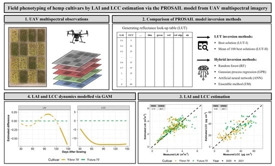
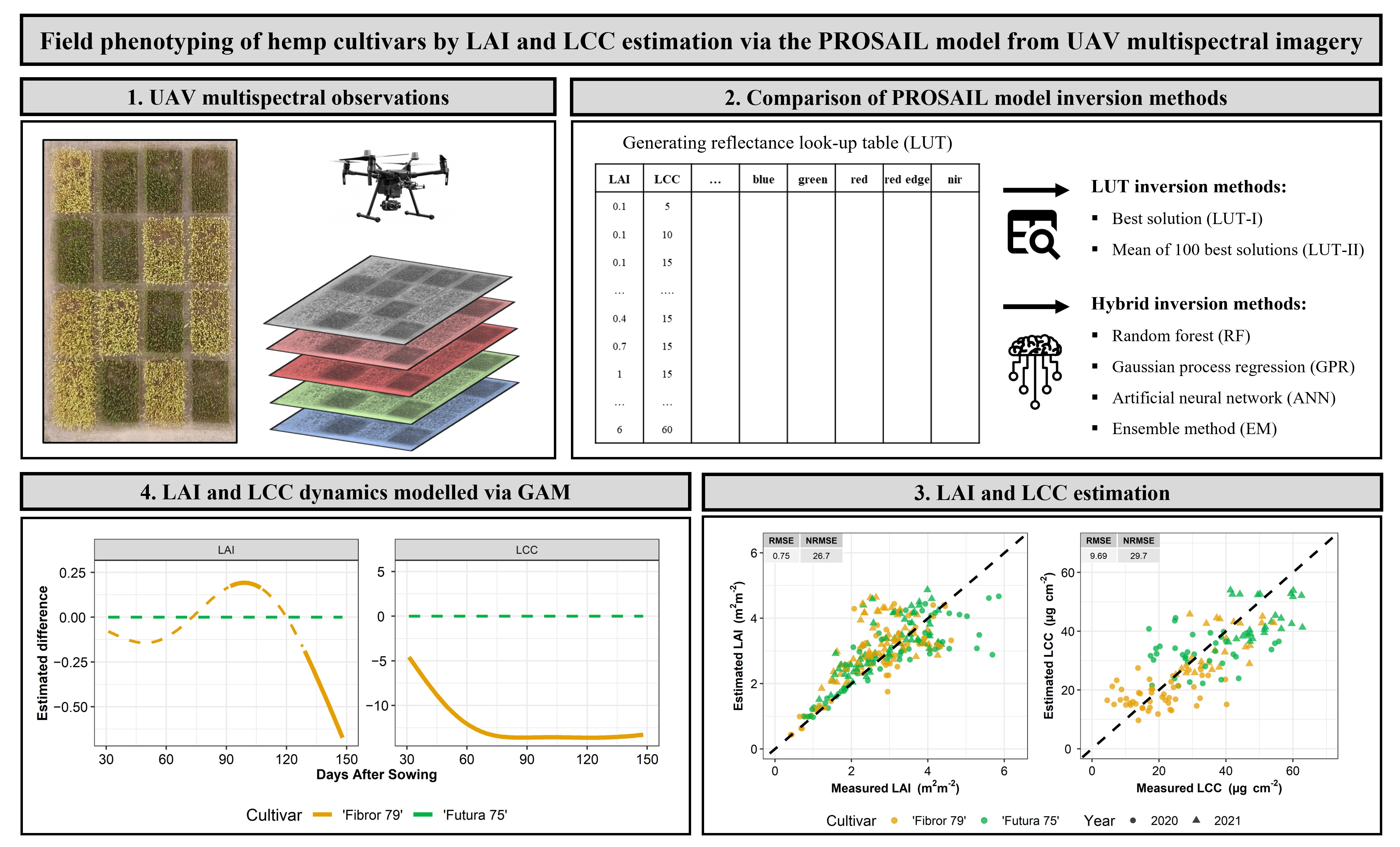
Comparison of PROSAIL Model Inversion Methods for Estimating Leaf Chlorophyll Content and LAI Using UAV Imagery for Hemp Phenotyping

by
Giorgio Impollonia
1,2,*,
Michele Croci
1,2,
Henri Blandinières
1,
Andrea Marcone
1,2 and
Stefano Amaducci
1,2
1
Department of Sustainable Crop Production, Università Cattolica del Sacro Cuore, 29122 Piacenza, Italy
2
Remote Sensing and Spatial Analysis Research Center (CRAST), Università Cattolica del Sacro Cuore, 29122 Piacenza, Italy
*
Author to whom correspondence should be addressed.
Remote Sens. 2022, 14(22), 5801; https://doi.org/10.3390/rs14225801
Submission received: 28 September 2022 / Revised: 12 November 2022 / Accepted: 15 November 2022 / Published: 17 November 2022
(This article belongs to the Special Issue UAS Technology and Applications in Precision Agriculture)

Abstract

:
Unmanned aerial vehicle (UAV) remote sensing was used to estimate the leaf area index (LAI) and leaf chlorophyll content (LCC) of two hemp cultivars during two growing seasons under four nitrogen fertilisation levels. The hemp traits were estimated by the inversion of the PROSAIL model from UAV multispectral images. The look-up table (LUT) and hybrid regression inversion methods were compared. The hybrid methods performed better than LUT methods, both for LAI and LCC, and the best accuracies were achieved by random forest for the LAI (0.75 m2 m−2 of RMSE) and by Gaussian process regression for the LCC (9.69 µg cm−2 of RMSE). High-throughput phenotyping was carried out by applying a generalised additive model to the time series of traits estimated by the PROSAIL model. Through this approach, significant differences in LAI and LCC dynamics were observed between the two hemp cultivars and between different levels of nitrogen fertilisation.

Graphical Abstract

1. Introduction

Interest in hemp (Cannabis sativa L.) cultivation, which is expanding internationally [1], is related to its high yield potential as this crop was reported to produce up to 20 Mg ha−1 of dry aboveground biomass in a few months of cultivation in given environments [2,3,4]. Additionally, hemp does not require phytosanitary products, it has low fertilisation requirements [5], and its integration into crop rotation systems can disrupt the weeds and disease cycles, increasing the sustainability of agrosystems [6]. All these features cause hemp to be an ideal crop in the frame of the expanding bioeconomy, by providing biomass for various low and high value bio-based applications (e.g., building materials, specialty papers, composite materials) [7]. Furthermore, not only hemp produces raw material for a wide range of bio-based applications, but it also produces seeds for food applications [1,3], in this way avoiding issues linked to indirect land use change. Despite the large interest in hemp, its cultivation has not significantly expanded in recent years due to legislative issues in link with the presence of psychoactive phyto-cannabinoids, but also due to limited innovation along the whole value chain [8]. In a recent EU project (MultiHemp), for the first time, innovative biotechnological tools have been applied for hemp breeding, but, so far, the management of hemp cultivation and the monitoring of its growth have not benefitted from the application of innovative precision agriculture technologies [9].
Unmanned aerial vehicle (UAV) remote sensing is a precision agriculture technology widely used to monitor crop growth [10,11]. UAV remote sensing platforms acquire a large volume of spectral data with high spatial and temporal resolutions, which are needed for applications in both precision agriculture [12] and high-throughput phenotyping (HTP) in the frame of breeding programs [13,14]. The spectral data acquired from the UAV HTP platforms are used to estimate crop traits during the growing season [15,16]. The leaf area index (LAI) and leaf chlorophyll content (LCC) are among the most important crop traits estimated in HTP applications [17,18]. The spatial and temporal information on LAI and LCC are usually regarded as relevant traits to monitor the status of crop growth [19,20]. Two main methods are used to estimate LAI and LCC using spectral data via remote sensing: (i) statistical methods such as linear regression or machine learning and (ii) physical methods based on radiative transfer models (RTMs) inversion. RTM-based methods have the advantage of overcoming the problem of lack of transferability and they minimise the reliance on in situ data over the statistical methods, which are site-specific [21]. The good reproducibility across environments makes RTMs particularly interesting for phenotyping applications, when field trials are carried out at multiple locations, in multiple years, and involving several genotypes. One of the most popular RTMs is the PROSAIL model [22], which simulates the canopy reflectance by combining the leaf PROSPECT model [23] and the canopy SAIL model [24]. Two main methods are commonly used for the PROSAIL model inversion: (i) look-up tables (LUTs) [25,26] based on a cost function and (ii) hybrid regression method [27] based on machine learning techniques such as artificial neural network (ANN) [28], Gaussian process regression (GPR) [29], and random forest (RF) [30]. The hybrid methods combine elements of statistical and physical methods using RTM-generated data to train machine learning (ML) algorithms. These algorithms enable the description of a non-linear relationship between the simulated canopy reflectance and relevant crop traits [31]. On the contrary, the LUT methods use a cost function to find the solution, i.e., the input parameters combination corresponding to the RTMs simulated canopy reflectance that most closely resembles the measured one [27]. However, the diverse combinations of crop traits can generate similar canopy reflectance causing the ill-posed problem of the PROSAIL model inversion [32]. To solve the ill-posed problem, to which no unique solution can be found, several strategies have been proposed, such as the use of multiple solutions (instead of the single best solution) [33,34] and the use of a priori knowledge on the ranges of input parameters [35]. Recently, several studies have demonstrated that the coupling of UAV remote sensing and the PROSAIL model provides reliable estimations of crop traits for HTP purposes, such as LAI and LCC [36,37,38,39,40]. However, these studies only evaluated the ability of the PROSAIL model to estimate crop traits, without characterising the dynamic of crop traits evolution along the growing season using the values estimated by the PROSAIL model. On the contrary, Impollonia et al. [41] and Antonucci et al. [42] demonstrated that the HTP of seasonal dynamic of crop traits can be characterised by combining multiple UAV observations, estimation models (i.e., machine learning and PROSAIL model), and a generalised additive model (GAM). The advantage of using the GAM in comparison to the use of smoothing functions is that the interactions of the variables can be used for fitting the models. These interactions are particularly important for multi-seasonal time series, which are typical of HTP field trials.
In this context, the main goal of this study was to evaluate the introduction of these innovative precision agriculture technologies for the monitoring and management of hemp cultivation, particularly HTP applications. In particular, in this study, UAV-based remote sensing technology were used: (i) to estimate hemp traits (LAI and LCC) and to compare two inversion methods of the PROSAIL model: LUT and hybrid regression methods and (ii) to characterise the dynamics of LAI and LCC of two contrasting hemp cultivars (a yellow and a green cultivar) under different nitrogen fertilisation levels via GAM.

2. Materials and Methods

2.1. Experimental Design

The field experiments were conducted at the CERZOO research centre (45°00′11.70″N, 9°42′35.39″E) in the province of Piacenza (NW Italy) during the years 2020 and 2021 (Figure 1). Two cultivars were used: “Futura 75”, a conventional green one, and “Fibror 79”, a yellow-stalked one, both having been developed and provided by Hemp-it (France). The seeds were sown on the 6th and on the 9th of April, in 2020 and 2021, respectively. The sowing density and depth were of about 45 kg ha−1 and 3 cm, respectively. The experimental layout was a complete randomised block design with four levels of nitrogen fertilisation: 0, 25, 50, and 100 kgN ha−1, with four replicates for a total of n = 32 plots (Figure 1).

2.2. Crop Measurements

During the vegetative growth, four georeferenced measurements of leaf area index (LAI) were performed, in each growing season (total n = 256). For each of these 256 measurements, five-to-six LAI measures were performed in a one-meter square quadrat with a ceptometer (AccuPAR LP-80, Decagon Devices, Inc., Pullman, WA, USA) between 12 p.m. and 2 p.m. (at zenith). This one-meter square quadrat was subsequently sampled in the frame of another experiment for yield determination (Figure 1). At the same time (Figure 2), the leaf mass per area (LMA) and equivalent water thickness (EWT) were determined from all the leaves of a three-to-five plant sample. The leaves were separated from the stems, weighted, and transferred to a fridge at −18 °C. The leaf surface was determined by scanning the leaves that were subsequently oven dried at 65 °C and weighted. The LMA (g cm−2) and EWT (g cm−2) were calculated as the ratio of the dry weight (LMA) or of the water weight (EWT) of the leaves to their surface. To determine the leaf chlorophyll content (LCC), additional leaf samples were collected at the top of the canopy, at three sampling times in 2020 and two in 2021 (total n = 160) (Figure 2). After collection, the samples were quickly stored in ice and transported to a −18 °C fridge up to analysis. The LCC was measured following the methods reported by Ritchie [43] and Warren [44].

2.3. UAV Multispectral Observations

The unmanned aerial vehicle (UAV) DJI Matrice 210 RTK was used in the experiment. The UAV was equipped with a MicaSense RedEdge-MX camera that acquired the images in five spectral bands (Table 1). The UAV observations were carried out at the same time as the crop measurements (Figure 2) and other UAV supplementary observations (i.e., UAV observations with no corresponding crop measurements) were also carried out to improve the analysis of the crop trait dynamics derived from multiple UAV observations as suggested by Impollonia et al. [41]. The UAV flight altitude was 50 m above ground level, the flight speed was set at 3 m s−1, and the ground sampling distance was 2.78 cm. The lateral and forward overlap was set at 75% and at 80% of the images, respectively. The reflectance panel provided by MicaSense and the light sensor mounted at the top of the UAV were used for the radiometric calibration of the images. Pix4D mapper software was used for radiometric calibration and orthomosaic generation. The experimental designs were drafted in AutoCAD and subsequently georeferenced using QGIS software. On the same position as the ceptometer measurements and after the UAV flight, destructive samplings were performed in the frame of another study. One-meter square polygons corresponding to the position of these destructive samplings were draft in AutoCAD and georeferenced to extract the mean values of spectral data of each plot, for the validation of the inversion PROSAIL model. Therefore, for the time series analysis based on multiple UAV observations, the sampled quadrats were subtracted from the experimental designs to eliminate the noise caused by these destructive measurements on the multispectral images as shown in Figure 1.

2.4. PROSAIL Model

The leaf area index (LAI) and leaf chlorophyll content (LCC) of hemp cultivars were estimated by the inversion of the PROSAIL model. The PROSAIL model combines the PROSPECT and SAIL models, simulating the canopy reflectance from 400 to 2500 nm. The leaf parameters and canopy parameters were used to simulate the leaves’ optical properties (PROSPECT model) and the bidirectional reflectance of the canopy (SAIL model). The leaf structure parameter (N, i.e., internal structure parameter of the leaf mesophyll), leaf chlorophyll content (LCC), leaf equivalent water thickness (EWT), and leaf mass per area (LMA) parameters were used to simulate the optical properties of leaves (PROSPECT model). The leaf area index (LAI), average leaf inclination angle (ALIA), hotspot parameter (hot), solar zenith angle (tts), observer zenith angle (tto), and relative azimuth angle (psi) parameters were used to simulate the bidirectional reflectance of canopy (SAIL model) (Table 2). The soil reflectance from 400 to 2500 nm was also considered in the PROSAIL model to characterise the soil backgrounds. However, the soil reflectance in this wavelength interval cannot be acquired by the UAV multispectral camera used in the present work and therefore it was retrieved from the database “ICRAF-ISRIC Soil VNIR Spectral Library” of the Soil Information System (ISIS) of the International Soil Reference and Information Centre (ISRIC), as this includes the soil reflectance from 400 to 2500 nm. The retrieval of the soil reflectance was performed firstly by the resampling of soils reflectance measured in Italy and found in the soil database, based on UAV multispectral camera characteristics (Table 1). Then, a calculation of the differences of soils reflectance measured in soils from Italy found in the database and soil reflectance extracted in this study from five UAV multispectral images was made. Finally, the soil with the least difference in reflectance was used in the PROSAIL model. The canopy reflectance was simulated from PROSAIL model using the R package hsdar [45]. The spectral reflectance simulated were resampled based on a MicaSense RedEdge-MX characteristics camera (Table 1). The canopy and leaf parameter combinations and the spectral reflectance simulated by PROSAIL model are used for look-up table (LUT) generation. The LUT generated included 86,400 parameter combinations following the ranges (minimum and maximum) and the steps of the parameters summarised in Table 2. In order to reduce the ill-posed problem [35], the ranges of values for the leaf and canopy parameters were fixed on the base of in field measurements acquired during the two growing seasons. The ALIA range was set between 10 and 30 because of the planophile nature of the hemp canopy [46]. All parameter combinations used for LUT generation were considered for LAI and LCC estimation as the hemp cultivars evaluated in this study exhibited large differences in traits (e.g., high LAI and low LCC for “Fibror 79” and high LAI and high LCC for “Futura 75” at the end of the vegetative phase) throughout the whole growing season (e.g., low LAI and high LCC at the start of the growing season and low LAI and low LCC at the end of the growing season).

2.5. Inversion Methods of the PROSAIL Model

Two inversion methods were compared in this study: a look-up table method based on a cost function and a hybrid regression method based on machine learning techniques.

2.5.1. The Look-Up Table Inversion Method

The look-up table (LUT) was sorted using the cost function based on the root mean square error (RMSE) to find the solution to the inverse problem for the measured canopy reflectance [33,34]. The RMSEr cost function (Equation (1)), between the measured reflectance and the simulated reflectance found in the LUT, was calculated as:
RMSE r = i = 1 n ( R measured i R simulated i ) 2 n
where n is the number of spectral bands, which was equal to five in the present work (blue, green, red, red edge, and near-infrared), R m e a s u r e d i is the reflectance at spectral band i measured by the UAV, and R s i m u l a t e d i is the simulated reflectance at spectral band i in the LUT. Two LUT methods were tested to find the solution to the inversion problem: the first LUT method (single best solution) was determined as the set of input parameters corresponding to the reflectance in the LUT that provides the smallest RMSEr; it will thereafter be referred to as LUT-I. However, this solution is not always the optimal one since it may not be unique (ill-posed problem). In order to reduce this problem, the second LUT method (multiple best solution), was determined using the mean value of parameters corresponding to the best 100 solutions (i.e., having the smallest sorted RMSEr) and it will thereafter be referred to as LUT-II.

2.5.2. The Hybrid Regression Inversion Method

The hybrid methods utilised the parameter combinations (y) and the simulated spectral reflectance (x) from the PROSAIL model, used for the LUT generation, to train machine learning regression models. Therefore, the hybrid regression methods allow replacing the field measurements needed to train nonparametric models, with the input parameters and the output simulated by the PROSAIL model [27]. This study evaluated different machine learning regression models: random forest (RF), Gaussian process regression (GPR), artificial neural network (ANN), and the ensemble method (EM) obtained combining RF, GPR, and ANN via stacking. The machine learning regression models were built using the caret and caretEnsemble R packages [47,48]. The structural hyperparameters of the machine learning regression models were optimised using a grid-searching method with cross-validation. The training dataset was created using a stratified random sampling method by LAI, LCC, and LMA value distribution of the LUT. The function of caretList was used for building the machine learning regression models using the method rf, gaussprRadial, and nnet, for RF, GPR, and ANN, respectively. The EM model was built using the function caretStack that finds a good linear combination of the models (RF, GPR, and ANN).

2.5.3. Comparison of Inversion Methods

The field measurements of LAI and LCC were used to validate the inversion methods of the PROSAIL model. The coefficient of determination (R2), the bias, the root mean square error (RMSE), and the normalised root mean square error (NRMSE) were used for inversion methods comparison. The bias was calculated using the mean of the difference between measured values and estimated values. The NRMSE was calculated using the mean of the measured values for normalising the RMSE [16]. These performance metrics were calculated for each season, for each cultivar, for each trait and for two different intervals of the traits. The LAI trait intervals investigated were LAI ≤ 3 m2 m−2 and LAI > 3 m2 m−2. The LCC trait intervals investigated were LCC ≤ 30 µg cm−2 and LCC > 30 µg cm−2.

2.5.4. Statistical Analysis of Inversion Methods

The non-parametric Friedman test was carried out to determine the best inversion method for LAI and LCC estimations among the six inversion methods (LUT-I, LUT-II, ANN, EM, GPR, and RF) as suggested by Demšar [49] and Kamir et al. [50]. A Nemenyi post hoc test was performed to compare pairwise performance differences [51]. These two statistical tests are based on ranks and they were performed using the NRMSE calculated for each combination of different cultivar, year, and nitrogen fertilisation levels. One hundred has been subtracted from the NRMSE values so that the low ranks indicate high performance and conversely high ranks indicate low performance [50]. Two inversion methods were stated as significantly different when the actual difference between their average rank was greater than the critical distance at the 95% confidence level. A critical distance diagram [49] was performed using the R package scmamp [52] and it was used to display the results of the Nemenyi post hoc test. The diagram showed the average rank of each inversion method and the critical distance.

2.6. GAM for Crop Phenotyping

The hemp cultivar traits were estimated from multiple UAV observations (supplementary observations were also considered) using the best inversion methods for each trait for phenotyping the dynamics of LAI and LCC and identifying differences among cultivars and nitrogen fertilisation levels. The time series of LAI and LCC values estimated from the PROSAIL model inversion were fitted against the day after sowing (DAS). The statistical analysis of the hemp traits time series was carried out via a generalised additive model (GAM). The GAM models were fitted in R package mgcv [53]. The fitted models used fixed factors such as season, block, cultivar, and nitrogen fertilisation levels and a smooth for DAS, based on season and on interaction of cultivars and nitrogen fertilisation levels.

3. Results

3.1. Data Distribution of LAI and LCC

The distribution of the leaf area index (LAI) and leaf chlorophyll content (LCC) measured during two years on green and yellow hemp cultivars is shown in Figure 3. Generally, “Futura 75” showed higher LAI and LCC values than “Fibror 79”. Regarding the LAI, “Fibror 79” and “Futura 75” showed the lowest (LAI < 1 m2 m−2) and the highest values (LAI > 5 m2 m−2) in 2020 while they showed a high frequency of the data in intermediate values (1.5 m2 m−2 < LAI < 4.5 m2 m−2) in 2021. Regarding the LCC, “Fibror 79” and “Futura 75” showed the lowest values (LCC < 18 µg cm−2 for “Fibror 79” and LCC < 40 µg cm−2 for “Futura 75”) in 2020 compared to the LCC values recorded in 2021.

3.2. Comparison of Inversion Methods for LAI Trait Estimation

The results of the comparison of the different methods used for the inversion of the PROSAIL model for the leaf area index (LAI) estimation is shown in Figure 4. Generally, the hybrid methods achieved better accuracies than the look-up table (LUT) methods. The random forest (RF) achieved the highest accuracy with 0.75 m2 m−2 of RMSE, 26.7% of NRMSE, and 0.55 of R2. The LUT-I showed greater accuracy than the LUT-II, which ranked last. The hybrid method with the worst accuracy was the ensemble method (EM) with 0.9 m2 m−2 of RMSE, 32.1% of NRMSE, 0.49 of R2, and −0.28 of bias (Figure 4). In Figure 4, the NRMSE values of the different methods, divided by years and cultivars, are reported. Generally, the RF was the best inversion method for both years and cultivars, except for 2020 where the ANN achieved the lowest NRMSE. Comparing the two years, “Fibror 79” displayed a higher variability of NRMSE than “Futura 75” (Figure 5). The different inversion methods were evaluated on two LAI intervals (Figure 5). In general, the inversion methods, when the LAI was ≤3 m2 m−2 were more accurate for “Futura 75” than “Fibror 79” while the opposite occurred when the LAI was >3 m2 m−2. The LUT methods and the RF achieved lower NRMSE than the GPR, ANN, and EM when the LAI was ≤3 m2 m−2 (Figure 5), while when the LAI was >3 m2 m−2, the hybrids methods performed better than the LUT methods. The Nemenyi post hoc test was performed to identify groups of inversion methods that significantly differed from one another (Figure 6). The inversion method with the highest average rank was RF, which was included in the first group with LUT-I, GPR, and ANN. The second group included LUT-I, GPR, ANN, EM, and LUT-II.

3.3. Comparison of Inversion Methods for LCC Trait Estimation

The results of the inversion methods of the PROSAIL model for the estimation of leaf chlorophyll content (LCC) are shown in Figure 7. The hybrid methods achieved better accuracies than the LUT methods. The Gaussian process regression (GPR) achieved the greatest accuracy with 9.69 µg cm−2 of RMSE, 29.7% of NRMSE, and 0.57 of R2. The hybrid method that showed the worst accuracy was the ANN with 10.52 µg cm−2 of RMSE, 32.3% of NRMSE, and 4.4 of bias (Figure 7). The NRMSE values of the different methods, divided by years and cultivars, are reported in Figure 8. Overall, the NRMSE values were lower in 2021 than in 2020 for both cultivars (Figure 8). The different methods were also evaluated on two LCC intervals (Figure 8). The NRMSE values were lower in LCC > 30 µg cm−2 than LCC ≤ 30 µg cm−2, particularly for “Futura 75”. The Nemenyi post hoc test was performed to identify groups of inversion methods that significantly differed from one another (Figure 9). The inversion method with the highest average rank was GPR. Only one group was identified so no significant difference was observed between inversion methods.

3.4. Dynamics of LAI and LCC of Hemp Cultivars

The best inversion methods, RF for LAI and GPR for LCC, were used to estimate the LAI and LCC of the two hemp cultivars using the spectral data acquired from multiple unmanned aerial vehicle (UAV) observations during 2020 and 2021 growing seasons. The maps of LAI and LCC estimated on 105 days after sowing (DAS) during the growing season 2020 are reported in Figure 10.
The generalised additive model (GAM) was applied to the time series of LAI and LCC estimated by the inversion of the PROSAIL model, with “Futura 75” as a reference for estimating significant differences among the hemp cultivars during the growing season (Figure 11). The estimated differences of LAI between “Futura 75” and “Fibror 79” were significant from 91 DAS to 108 DAS, with higher values of LAI for “Fibror 79” than for “Futura 75”, while higher values of LAI for “Futura 75” than for “Fibror 79” were observed from 129 DAS until the end of the growing season (Figure 11). Higher values of LAI were observed in “Futura 75” than “Fibror 79” during the early phases of the growing season (until 72 DAS), but no significant differences were observed. The estimated differences of LCC were significant throughout the whole growing season, with higher values of LCC for “Futura 75” than for “Fibror 79” (Figure 11). The estimated differences of LCC showed an increase from the start of the growing season up to 75 DAS (estimated difference of −13.5 µg cm−2) and remained constant afterward until the end of the growing season.

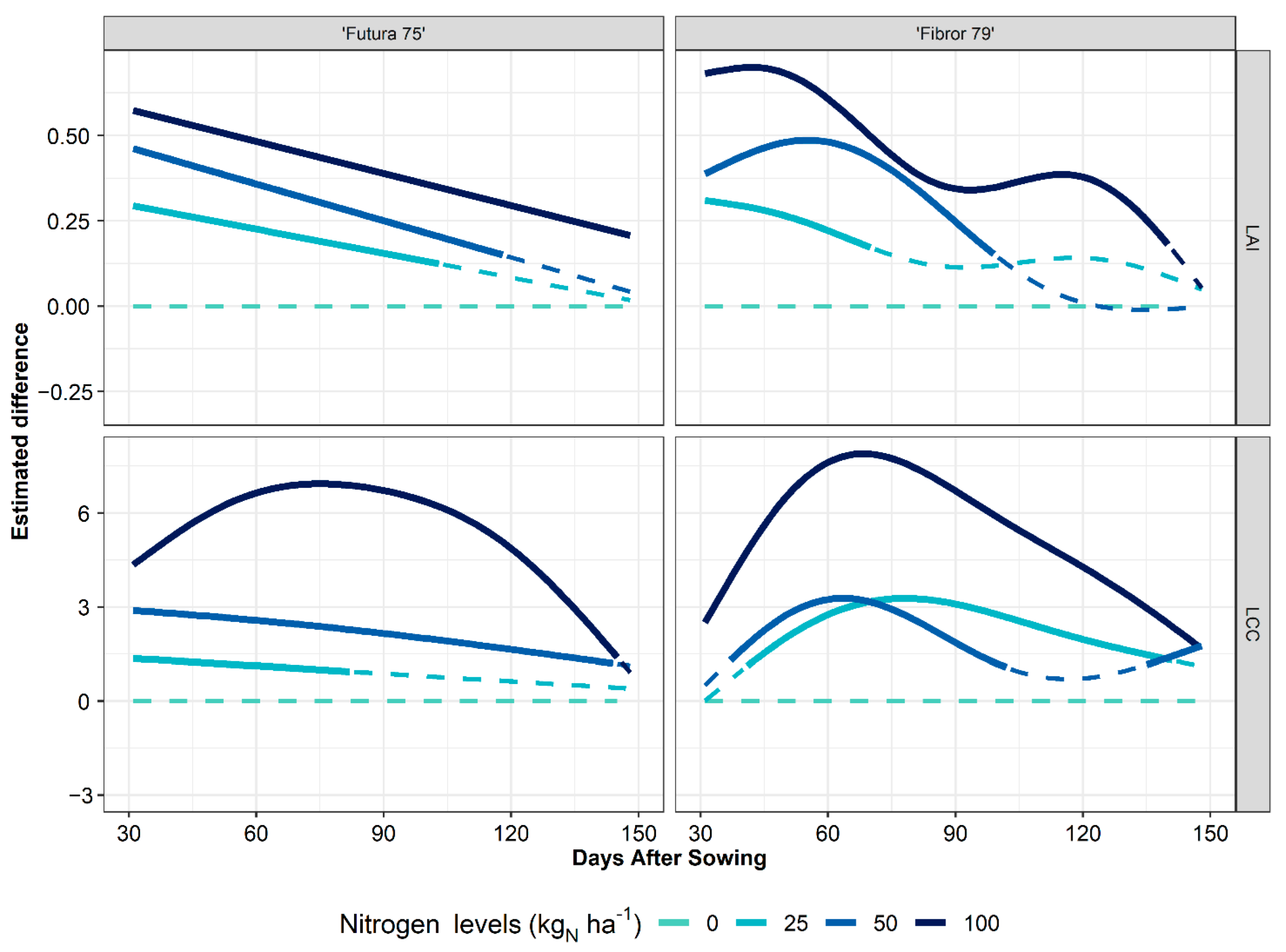
3.5. Effect of Nitrogen Fertilisation on LAI and LCC Dynamics

The GAM was also used to analyse the effect of nitrogen fertilisation on the dynamics of the LAI and LCC of the two hemp cultivars. The reference used for estimating significant differences among nitrogen levels for each cultivar was the lowest fertilisation dose, i.e., 0 kgN ha−1 (Figure 12). The analysis showed that the effect of nitrogen dose was significant for both cultivars and both traits. The largest estimated differences were observed with the highest nitrogen level and decreased proportionally to the nitrogen dose. The estimated differences of LAI were highest during early phases of the growing season and progressively decreased until the final harvest (Figure 12). Generally, the LCC showed the highest estimated differences at the end of the vegetative growth from 60 DAS to 90 DAS approximately, except for “Futura 75” at 25 and 50 kgN ha−1 nitrogen levels where the highest estimated differences were observed at the start of the vegetative growth. The LAI of “Futura 75” showed significant estimated differences throughout the whole growing season with 100 kgN ha−1 nitrogen level and from the start of the growing season until 118 DAS and 103 DAS with 50 kgN ha−1 and 25 kgN ha−1 nitrogen levels, respectively. The “Futura 75” LCC showed significant estimated differences from the start of the growing season until 144 DAS, 145 DAS, and 82 DAS with 100 kgN ha−1, 50 kgN ha−1, and 25 kgN ha−1 nitrogen levels, respectively (Figure 12). The LAI of “Fibror 79” showed significant estimated differences from the start of the growing season until 140 DAS, 99 DAS, and 70 DAS with 100 kgN ha−1, 50 kgN ha−1, and 25 kgN ha−1 nitrogen levels, respectively. “Fibror 79” LCC showed significant estimated differences throughout the whole growing season with 100 kgN ha−1 nitrogen levels, from the 37 DAS and 40 DAS until 102 DAS and 141 DAS with 50 kgN ha−1 and 25 kgN ha−1 nitrogen levels, respectively (Figure 12). Significant LCC estimated differences of “Fibror 79” were also observed for 50 kgN ha−1 nitrogen levels from 135 DAS to the end of the growing season.

4. Discussion

4.1. Evaluation of the Inversion Methods Accuracy for the Estimation of LAI and LCC

This study focused on UAV-based remote sensing estimation of hemp traits to phenotype two contrasting cultivars and to support the application of innovative precision agriculture. Multispectral data acquired from an unmanned aerial vehicle (UAV) in two growing seasons (2020 and 2021) were used to estimate the leaf area index (LAI) and leaf chlorophyll content (LCC) using inversion methods of the PROSAIL model.

4.1.1. Effects of Data Distribution on Accuracy of LAI and LCC Estimation

The UAV multispectral camera used in this study (MicaSense RedEdge-MX) includes five spectral bands and enabled a reliable estimation of LAI and LCC, achieving results comparable to those obtained in previous studies, conducted with both multispectral [38,39,40] and hyperspectral UAV cameras [36,54]. However, it remains difficult to compare the models’ accuracy achieved in different conditions (i.e., years and cultivars) or studies because the performance metrics such as RMSE and NRMSE depend on the data distribution (i.e., size, mean, and range of the traits) used for the validation of the models. For example, in this study, high differences of NRMSE values for LCC estimation were observed between years or LCC intervals. These results can be explained analysing the LCC distribution as, for example, in 2020, the higher NRMSE values can be caused by the high frequency of low LCC values in this year compared to 2021. In fact, the lowest accuracy of LCC estimation was observed ≤ 30 µg cm−2; this may have been caused by hemp blooming at the end of the season, as crop blooming has already been reported to affect reflectance data [40]. Analysing the accuracy of the LAI estimation, low accuracies were observed when the LAI was ≤3 m2 m−2 and this may have been caused by the interferences of the soil at low LAI values, which can affect the reflectance of the multispectral images from UAV, as observed by Xu et al. [55]. However, at LAI ≤ 3 m2 m−2, the high difference between measured and estimated LAI (Figure 3) were observed between 2 m2 m−2 and 3 m2 m−2 and this aspect could be explained by the difference of LAI accuracy in “Fibror 79” between 2020 (low values of NRMSE) and 2021 (high values of NRMSE), because in 2021 the LAI measured showed a high frequency of the values between 2 m2 m−2 and 3 m2 m−2.

4.1.2. Comparison of Hybrids and LUT Inversion Methods

Among the different inversion methods reported in the literature, this study compared two look-up table (LUT) methods based on the RMSEr cost function (LUT-I and LUT-II) and four hybrid regression methods based on machine learning techniques (RF, GPR, ANN, and EM) to identify the most accurate LAI and LCC estimation method. The results obtained with the LUT methods showed that the LUT-I method (single best solution) achieved a better accuracy than the LUT-II method (mean of 100 best solutions). The opposite results were reported for heterogenous grassland, by Darvishzadeh et al. [33], and for wheat, by Sehgal et al. [34]. Regarding hybrid methods, the best accuracies were achieved with random forest (RF) for LAI and Gaussian process regression (GPR) for LCC, which was also the most accurate method for estimating LCC in a study conducted on multi-crop by Verrelst et al. [56]. Low accuracies were achieved using the ensemble method (EM) for both LAI and LCC, which could be the consequence of the high correlation among the values predicted by the individual algorithms (RF, GPR, and ANN), as already reported by Kamir et al. [50].
In this study, the LAI estimation was generally more accurate than the estimation of the LCC. This confirms the difficulty of estimating LCC, which was already reported in previous studies [33,34,57] and that is the consequence of the poor signal propagation from leaf to canopy scale, as demonstrated by Asner [58]. Overall, estimation of the LAI and LCC was more accurate using hybrid methods than LUT ones, which is in agreement with what was reported by Fei et al. [59] and Zhang et al. [60], but not with the findings of Sehgal et al. [34] and Vohland et al. [61], who found that the LUT inversion methods were more accurate than the hybrid ones. Ali et al. [62], instead, did not find differences between the methods. This aspect was confirmed in this study using the critical distance diagram where few (for LAI) and no (for LCC) significant differences were observed, though RF for LAI and GPR for LCC ranked first. However, accuracy is not the only criteria to consider when selecting the inversion method of the PROSAIL model. For example, studies have focused on the inversion run time, showing that hybrid methods are faster in performing the inversion compared to LUT methods [27,62]. Therefore, these hybrid methods appear particularly pertinent for crop trait estimation for their accuracy and their fast inversion compared to LUT methods.

4.2. UAV Remote Sensing and GAM for Phenotyping the Dynamics of LAI and LCC

High-throughput phenotyping (HTP) obtained by the combination of multiple UAV observations, estimation models of crop traits, and generalised additive model (GAM) analysis, can characterise the dynamics of relevant crop traits [41,42]. This study focused on the application of UAV multispectral images for characterising LAI and LCC in hemp. The time series of the traits estimated (with the best method for each trait) were used to characterise two hemp cultivars (a green and a yellow one), grown with different nitrogen fertilisation levels, using a generalised additive model (GAM).

4.2.1. Hemp Cultivars Phenotyping

The use of GAM to compare the LAI dynamics of two hemp cultivars showed that the LAI of “Futura 75” tended to be higher (but not significantly) than that of “Fibror 79” in the early phases of the growing season. At the end of the vegetative phase, LAI was highest in “Fibror 79” and finally it became highest in “Futura 75” during the seed maturing phase (Figure 11). The highest LAI of “Futura 75” at the start of the growing season might indicate that its canopy developed more rapidly than that of “Fibror 79”. However, 90 days after sowing (DAS), the LAI of “Fibror 79” increased faster than that of “Futura 75” and became even significantly higher for 18 days (between 91 DAS and 108 DAS). This could be explained by the fact that “Fibror 79” is a cultivar that flowers slightly later (with about 4 days of delay according to the breeder) than “Futura 75”, hence the senescence of “Futura 75” starts sooner than for “Fibror 79”, explaining the observed dynamic of LAI estimated differences between both cultivars. These results are in accordance with Herppich et al. [63] who reported that the LAI peak of “Ivory” (the yellow cv.), a cultivar that flowers earlier than “Santhica 27” (the green cv.), was reached sooner than the LAI peak of “Santhica 27”. They also found that for the green cultivar “Santhica 27”, the LAI remained the highest for the rest of the growing season. After flowering, the same dynamics were observed in this study where the LAI of the green cultivar “Futura 75” was significantly higher than that of “Fibror 79” during the seed filling phase. This could be due to the higher nitrogen content in “Futura 75” leaves than in “Fibror 79” ones, in line with the statement of Thouminot [64], who stated that the yellow strain of hemp (i.e., “Fibror 79”) was due to a reduced capacity of nitrogen assimilation. Indeed, the dynamic of LCC observed in this study, linked to leaf nitrogen content [65], showed higher values for “Futura 75” than for “Fibror 79” throughout the whole growing season. The LCC estimated differences of the two hemp cultivars showed an increase from the start of the growing season until 75 DAS and then remained constant until the end of the growing season (Figure 11).

4.2.2. Effects of Nitrogen Fertilisation on Hemp Growth

In order to characterise the LAI and LCC dynamics of hemp cultivars, the nitrogen fertilisation effects were included in the GAM analysis. The nitrogen fertilisation had a significant effect on the LAI and LCC dynamics (Figure 12). As for the LAI, the higher estimated differences across the nitrogen fertilisation levels were observed in the early phases of the growing season for both cultivars. These results are in accordance with those reported by Seleiman et al. [66], who found that the nitrogen fertilisation treatments had a significant effect on the LAI of hemp only at the start of the growing season (44 DAS). The higher estimated differences of LAI between the nitrogen levels could be due to a greater nitrogen accumulation at the start of the growing season, as reported by Ivonyi et al. [67]. They found, for hemp, that the most intense phase of nitrogen accumulation occurred between 30 and 60 DAS, as 79% of the total amount of nitrogen had effectively been accumulated after 60 DAS, in accordance with Seleiman et al. [66]. This intense nitrogen uptake during the early phases of the growing season could explain the general increase of estimated differences of LCC until 60–80 DAS when a peak of LCC estimated differences occurred (Figure 12). The increase of nitrogen fertilisation led to increases in nitrogen uptake and accumulation by the crop, with a subsequent significant increase in LCC, as reported by Yang et al. [68]. This relation was also observed in this study, as LCC dynamics had higher values at increasing levels of nitrogen fertilisation. After flowering, the LCC estimated differences decreased with the start of the senescence stage and the start of the chlorophyll’s degradation.

5. Conclusions

This study demonstrated that hemp traits can be estimated with relatively good accuracy by the inversion of the PROSAIL model using multispectral images acquired by UAV. Generally, the hybrid methods performed better than LUT methods, both for LAI and LCC estimations, and the best accuracies were achieved by RF for estimating the LAI and by GPR for estimating LCC. Few significant differences for LAI estimation and no significant differences for LCC estimation were observed between the hybrid and LUT methods. However, if the same accuracy is achieved by hybrids and LUT methods, it is preferable to use the hybrid methods for their fast inversion compared to LUT methods. The HTP of the crops can be carried out by applying the GAM to the time series of traits estimated by the inversion of the PROSAIL model from multiple multispectral UAV observations. The GAM analysis showed differences in the LAI and LCC dynamics between two hemp cultivars with contrasting phenotypes. In particular, the dynamic of LAI along the growing season was different between the two cultivars, with “Futura 75” having a slightly faster increment of LAI than “Fibror 79” early in the season, while the opposite occurred at the end of the vegetative growth. The two cultivars also clearly differed in terms of estimated LCC, with “Futura 75” consistently having the highest LCC. Nitrogen fertilisation also had a significant effect on the dynamics of both traits, with increasing levels of nitrogen leading to increments of LAI and LCC. HTP based on UAV remote sensing proved to be a powerful tool to estimate crop traits and to improve our understanding of the traits’ dynamics of contrasting cultivars throughout the whole growing season. These innovative precision agriculture technologies can contribute to the development of the hemp sector; for example, enabling the HTP of different genotypes for drought tolerance characterisation in the frame of breeding programs or by allowing a precise monitoring and an efficient management of hemp’s cultivation.

Author Contributions

Conceptualization, G.I. and M.C.; methodology, G.I. and M.C.; software, G.I. and M.C.; formal analysis, G.I.; investigation, G.I., M.C. A.M., and H.B.; resources, S.A.; data curation, G.I. and H.B.; writing—original draft preparation, G.I.; writing—review and editing, H.B. and S.A.; visualization, G.I.; funding acquisition, S.A. All authors have read and agreed to the published version of the manuscript.

Funding

This study is part of the GRACE project, which has received funding from the Bio-based Industries Joint Undertaking (JU) under the European Union’s Horizon 2020 research and innovation programme under grant agreement No 745012. The JU receives support from the European Union’s Horizon 2020 research and innovation programme and the Bio-based Industries Consortium.

Data Availability Statement

The data that support the findings of this work are available from the corresponding author upon reasonable request.

Conflicts of Interest

The authors declare no conflict of interest.

References

  1. Amaducci, S.; Scordia, D.; Liu, F.H.; Zhang, Q.; Guo, H.; Testa, G.; Cosentino, S.L. Key cultivation techniques for hemp in Europe and China. Ind. Crops Prod. 2015, 68, 2–16. [Google Scholar] [CrossRef]
  2. Struik, P.C.; Amaducci, S.; Bullard, M.J.; Stutterheim, N.C.; Venturi, G.; Cromack, H.T.H. Agronomy of fibre hemp (Cannabis Sativa L.) in Europe. Ind. Crops Prod. 2000, 11, 107–118. [Google Scholar] [CrossRef]
  3. Tang, K.; Struik, P.C.; Yin, X.; Thouminot, C.; Bjelková, M.; Stramkale, V.; Amaducci, S. Comparing hemp (Cannabis Sativa L.) cultivars for dual-purpose production under contrasting environments. Ind. Crops Prod. 2016, 87, 33–44. [Google Scholar] [CrossRef]
  4. Burczyk, H.; Grabowska, L.; Kołodziej, J.; Strybe, M. Industrial hemp as a raw material for energy production. J. Ind. Hemp 2008, 13, 37–48. [Google Scholar] [CrossRef]
  5. Tang, K.; Struik, P.C.; Yin, X.; Calzolari, D.; Musio, S.; Thouminot, C.; Bjelková, M.; Stramkale, V.; Magagnini, G.; Amaducci, S. A comprehensive study of planting density and nitrogen fertilization effect on dual-purpose hemp (Cannabis Sativa L.) cultivation. Ind. Crops Prod. 2017, 107, 427–438. [Google Scholar] [CrossRef]
  6. Blandinières, H.; Amaducci, S. Agronomy and ecophysiology of hemp cultivation. In Cannabis/Hemp for Sustainable Agriculture and Materials; Springer: Singapore, 2022; pp. 89–125. [Google Scholar]
  7. Müssig, J.; Amaducci, S.; Bourmaud, A.; Beaugrand, J.; Shah, D.U. Transdisciplinary top-down review of hemp fibre composites: From an advanced product design to crop variety selection. Compos. Part C Open Access 2020, 2, 100010. [Google Scholar] [CrossRef]
  8. Venturi, P.; Amaducci, S.; Amaducci, M.T.; Venturi, G. Interaction between agronomic and mechanical factors for fiber crops harvesting: Italian results-note II. hemp. J. Nat. Fibers 2007, 4, 83–97. [Google Scholar] [CrossRef]
  9. Müssig, J.; Haag, K.; Musio, S.; Bjelková, M.; Albrecht, K.; Uhrlaub, B.; Wang, S.; Wieland, H.; Amaducci, S. Biobased ‘mid-performance’ composites using losses from the hackling process of long hemp—A feasibility study as part of the development of a biorefinery concept. Ind. Crops Prod. 2020, 145, 111938. [Google Scholar] [CrossRef]
  10. Sishodia, R.P.; Ray, R.L.; Singh, S.K. Applications of remote sensing in precision agriculture: A review. Remote Sens. 2020, 12, 3136. [Google Scholar] [CrossRef]
  11. de Castro, A.I.; Shi, Y.; Maja, J.M.; Peña, J.M. UAVs for vegetation monitoring: Overview and recent scientific contributions. Remote Sens. 2021, 13, 2139. [Google Scholar] [CrossRef]
  12. Segarra, J.; Buchaillot, M.L.; Araus, J.L.; Kefauver, S.C. Remote sensing for precision agriculture: Sentinel-2 improved features and applications. Agronomy 2020, 10, 641. [Google Scholar] [CrossRef]
  13. Guo, W.; Carroll, M.E.; Singh, A.; Swetnam, T.L.; Merchant, N.; Sarkar, S.; Singh, A.K.; Ganapathysubramanian, B. UAS-based plant phenotyping for research and breeding applications. Plant Phenomics 2021, 2021, 9840192. [Google Scholar] [CrossRef] [PubMed]
  14. Yang, G.; Liu, J.; Zhao, C.; Li, Z.Z.; Huang, Y.; Yu, H.; Xu, B.; Yang, X.; Zhu, D.; Zhang, X.; et al. Unmanned aerial vehicle remote sensing for field-based crop phenotyping: Current status and perspectives. Front. Plant Sci. 2017, 8, 1111. [Google Scholar] [CrossRef] [Green Version]
  15. Blancon, J.; Dutartre, D.; Tixier, M.-H.H.; Weiss, M.; Comar, A.; Praud, S.; Baret, F. A high-throughput model-assisted method for phenotyping maize green leaf area index dynamics using unmanned aerial vehicle imagery. Front. Plant Sci. 2019, 10, 685. [Google Scholar] [CrossRef] [PubMed]
  16. Impollonia, G.; Croci, M.; Ferrarini, A.; Brook, J.; Martani, E.; Blandinières, H.; Marcone, A.; Awty-Carroll, D.; Ashman, C.; Kam, J.; et al. UAV remote sensing for high-throughput phenotyping and for yield prediction of miscanthus by machine learning techniques. Remote Sens. 2022, 14, 2927. [Google Scholar] [CrossRef]
  17. Potgieter, A.B.; George-Jaeggli, B.; Chapman, S.C.; Laws, K.; Suárez Cadavid, L.A.; Wixted, J.; Watson, J.; Eldridge, M.; Jordan, D.R.; Hammer, G.L. Multi-spectral imaging from an unmanned aerial vehicle enables the assessment of seasonal leaf area dynamics of sorghum breeding lines. Front. Plant Sci. 2017, 8, 1532. [Google Scholar] [CrossRef]
  18. Xie, C.; Yang, C. A Review on plant high-throughput phenotyping traits using UAV-based sensors. Comput. Electron. Agric. 2020, 178, 105731. [Google Scholar] [CrossRef]
  19. Duan, B.; Liu, Y.; Gong, Y.; Peng, Y.; Wu, X.; Zhu, R.; Fang, S. Remote estimation of rice LAI based on fourier spectrum texture from UAV image. Plant Methods 2019, 15, 124. [Google Scholar] [CrossRef] [Green Version]
  20. Xu, Y.; Shrestha, V.; Piasecki, C.; Wolfe, B.; Hamilton, L.; Millwood, R.J.; Mazarei, M.; Stewart, C.N. Sustainability trait modeling of field-grown switchgrass (Panicum Virgatum) using UAV-based imagery. Plants 2021, 10, 2726. [Google Scholar] [CrossRef]
  21. Atzberger, C.; Darvishzadeh, R.; Immitzer, M.; Schlerf, M.; Skidmore, A.; le Maire, G. Comparative analysis of different retrieval methods for mapping grassland leaf area index using airborne imaging spectroscopy. Int. J. Appl. Earth Obs. Geoinf. 2015, 43, 19–31. [Google Scholar] [CrossRef]
  22. Berger, K.; Atzberger, C.; Danner, M.; D’Urso, G.; Mauser, W.; Vuolo, F.; Hank, T.; D’Urso, G.; Mauser, W.; Vuolo, F.; et al. Evaluation of the PROSAIL model capabilities for future hyperspectral model environments: A review study. Remote Sens. 2018, 10, 85. [Google Scholar] [CrossRef] [Green Version]
  23. Jacquemoud, S.; Baret, F. PROSPECT: A model of leaf optical properties spectra. Remote Sens. Environ. 1990, 34, 75–91. [Google Scholar] [CrossRef]
  24. Verhoef, W. Light scattering by leaf layers with application to canopy reflectance modeling: The SAIL model. Remote Sens. Environ. 1984, 16, 125–141. [Google Scholar] [CrossRef] [Green Version]
  25. Verrelst, J.; Rivera, J.P.; Leonenko, G.; Alonso, L.; Moreno, J.J. Optimizing LUT-based RTM inversion for semiautomatic mapping of crop biophysical parameters from Sentinel-2 and -3 data: Role of cost functions. IEEE Trans. Geosci. Remote Sens. 2014, 52, 257–269. [Google Scholar] [CrossRef]
  26. Verrelst, J.; Rivera, J.P.; Veroustraete, F.; Muñoz-Marí, J.; Clevers, J.G.P.W.; Camps-Valls, G.; Moreno, J. Experimental Sentinel-2 LAI estimation using parametric, non-parametric and physical retrieval methods—A comparison. ISPRS J. Photogramm. Remote Sens. 2015, 108, 260–272. [Google Scholar] [CrossRef]
  27. Verrelst, J.; Malenovský, Z.; Van der Tol, C.; Camps-Valls, G.; Gastellu-Etchegorry, J.-P.; Lewis, P.; North, P.; Moreno, J. Quantifying vegetation biophysical variables from imaging spectroscopy data: A review on retrieval methods. Surv. Geophys. 2019, 40, 589–629. [Google Scholar] [CrossRef] [PubMed] [Green Version]
  28. Atzberger, C. Inverting the PROSAIL canopy reflectance model using neural nets trained on streamlined databases. J. Spectr. Imaging 2010, 1, a2. [Google Scholar] [CrossRef] [Green Version]
  29. Verrelst, J.; Dethier, S.; Rivera, J.P.; Munoz-Mari, J.; Camps-Valls, G.; Moreno, J. Active learning methods for efficient hybrid biophysical variable retrieval. IEEE Geosci. Remote Sens. Lett. 2016, 13, 1012–1016. [Google Scholar] [CrossRef]
  30. Doktor, D.; Lausch, A.; Spengler, D.; Thurner, M. Extraction of plant physiological status from hyperspectral signatures using machine learning methods. Remote Sens. 2014, 6, 12247–12274. [Google Scholar] [CrossRef] [Green Version]
  31. Machwitz, M.; Pieruschka, R.; Berger, K.; Schlerf, M.; Aasen, H.; Fahrner, S.; Jiménez-Berni, J.; Baret, F.; Rascher, U. Bridging the gap between remote sensing and plant phenotyping—Challenges and opportunities for the next generation of sustainable agriculture. Front. Plant Sci. 2021, 12, 2334. [Google Scholar] [CrossRef]
  32. Atzberger, C. Object-based retrieval of biophysical canopy variables using artificial neural nets and radiative transfer models. Remote Sens. Environ. 2004, 93, 53–67. [Google Scholar] [CrossRef]
  33. Darvishzadeh, R.; Skidmore, A.; Schlerf, M.; Atzberger, C. Inversion of a radiative transfer model for estimating vegetation LAI and Chlorophyll in a heterogeneous grassland. Remote Sens. Environ. 2008, 112, 2592–2604. [Google Scholar] [CrossRef]
  34. Sehgal, V.K.; Chakraborty, D.; Sahoo, R.N. Inversion of radiative transfer model for retrieval of wheat biophysical parameters from broadband reflectance measurements. Inf. Process. Agric. 2016, 3, 107–118. [Google Scholar] [CrossRef] [Green Version]
  35. Meroni, M.; Colombo, R.; Panigada, C. Inversion of a radiative transfer model with hyperspectral observations for LAI mapping in poplar plantations. Remote Sens. Environ. 2004, 92, 195–206. [Google Scholar] [CrossRef]
  36. Duan, S.-B.B.; Li, Z.-L.L.; Wu, H.; Tang, B.-H.H.; Ma, L.; Zhao, E.; Li, C. Inversion of the PROSAIL model to estimate leaf area index of maize, potato, and sunflower fields from unmanned aerial vehicle hyperspectral data. Int. J. Appl. Earth Obs. Geoinf. 2014, 26, 12–20. [Google Scholar] [CrossRef]
  37. Jay, S.; Maupas, F.; Bendoula, R.; Gorretta, N. Retrieving LAI, Chlorophyll and nitrogen contents in sugar beet crops from multi-angular optical remote sensing: Comparison of vegetation indices and PROSAIL inversion for field phenotyping. F. Crop. Res. 2017, 210, 33–46. [Google Scholar] [CrossRef] [Green Version]
  38. Sun, B.; Wang, C.; Yang, C.; Xu, B.; Zhou, G.; Li, X.; Xie, J.; Xu, S.; Liu, B.; Xie, T.; et al. Retrieval of rapeseed leaf area index using the PROSAIL model with canopy coverage derived from UAV images as a correction parameter. Int. J. Appl. Earth Obs. Geoinf. 2021, 102, 102373. [Google Scholar] [CrossRef]
  39. Zhu, W.; Sun, Z.; Huang, Y.; Lai, J.; Li, J.; Zhang, J.; Yang, B.; Li, B.; Li, S.; Zhu, K.; et al. Improving field-scale wheat LAI retrieval based on UAV remote-sensing observations and optimized VI-LUTs. Remote Sens. 2019, 11, 2456. [Google Scholar] [CrossRef] [Green Version]
  40. Wan, L.; Zhang, J.; Dong, X.; Du, X.; Zhu, J.; Sun, D.; Liu, Y.; He, Y.; Cen, H. Unmanned aerial vehicle-based field phenotyping of crop biomass using growth traits retrieved from PROSAIL model. Comput. Electron. Agric. 2021, 187, 106304. [Google Scholar] [CrossRef]
  41. Impollonia, G.; Croci, M.; Martani, E.; Ferrarini, A.; Kam, J.; Trindade, L.M.; Clifton-Brown, J.; Amaducci, S. Moisture content estimation and senescence phenotyping of novel miscanthus hybrids combining UAV-based remote sensing and machine learning. GCB Bioenergy 2022, 14, 639–656. [Google Scholar] [CrossRef]
  42. Antonucci, G.; Impollonia, G.; Croci, M.; Potenza, E.; Marcone, A.; Amaducci, S. Evaluating biostimulants via high-throughput field phenotyping: Biophysical traits retrieval through PROSAIL inversion. Smart Agric. Technol. 2023, 3, 100067. [Google Scholar] [CrossRef]
  43. Ritchie, R.J. Consistent sets of spectrophotometric Chlorophyll equations for acetone, methanol and ethanol solvents. Photosynth. Res. 2006, 89, 27–41. [Google Scholar] [CrossRef] [PubMed]
  44. Warren, C.R. Rapid measurement of chlorophylls with a microplate reader. J. Plant Nutr. 2008, 31, 1321–1332. [Google Scholar] [CrossRef]
  45. Lehnert, L.W.; Meyer, H.; Obermeier, W.A.; Silva, B.; Regeling, B.; Bendix, J. Hyperspectral data analysis in R: The Hsdar Package. J. Stat. Softw. 2019, 89, 1–23. [Google Scholar] [CrossRef] [Green Version]
  46. Meijer, W.J.M.; van der Werf, H.M.G.; Mathijssen, E.W.J.M.; van den Brink, P.W.M. Constraints to dry matter production in fibre hemp (Cannabis Sativa L.). Eur. J. Agron. 1995, 4, 109–117. [Google Scholar] [CrossRef]
  47. Kuhn, M. Building predictive models in R using the caret package. J. Stat. Softw. 2008, 28, 1–26. [Google Scholar] [CrossRef] [Green Version]
  48. Mayer, Z. A Brief Introduction to CaretEnsemble 2019. Available online: https://cran.r-project.org/web/packages/caretEnsemble/vignettes/caretEnsemble-intro.html (accessed on 12 December 2019).
  49. Demšar, J. Statistical comparisons of classifiers over multiple data sets. J. Mach. Learn. Res. 2006, 7, 1–30. [Google Scholar]
  50. Kamir, E.; Waldner, F.; Hochman, Z. Estimating wheat yields in australia using climate records, satellite image time series and machine learning methods. ISPRS J. Photogramm. Remote Sens. 2020, 160, 124–135. [Google Scholar] [CrossRef]
  51. Nemenyi, P. Distribution-Free Multiple Comparisons. Ph.D. Thesis, Princeton University, Princeton, NJ, USA, 1963. [Google Scholar]
  52. Calvo, B.; Santafe, G. Statistical comparison of multiple algorithms in multiple problems. R J. 2016, 8, 1–8. [Google Scholar] [CrossRef] [Green Version]
  53. Wood, S.N. Generalized Additive Models; Chapman and Hall/CRC: Boca Raton, FL, USA, 2017; ISBN 9781315370279. [Google Scholar]
  54. Wang, L.; Chen, S.; Peng, Z.; Huang, J.; Wang, C.; Jiang, H.; Zheng, Q.; Li, D. Phenology effects on physically based estimation of paddy rice canopy traits from UAV hyperspectral imagery. Remote Sens. 2021, 13, 1792. [Google Scholar] [CrossRef]
  55. Xu, X.Q.Q.; Lu, J.S.S.; Zhang, N.; Yang, T.C.C.; He, J.Y.Y.; Yao, X.; Cheng, T.; Zhu, Y.; Cao, W.X.X.; Tian, Y.C.C. Inversion of rice canopy chlorophyll content and leaf area index based on coupling of radiative transfer and bayesian network models. ISPRS J. Photogramm. Remote Sens. 2019, 150, 185–196. [Google Scholar] [CrossRef]
  56. Verrelst, J.; Muñoz, J.; Alonso, L.; Delegido, J.; Rivera, J.P.; Camps-Valls, G.; Moreno, J. Machine learning regression algorithms for biophysical parameter retrieval: Opportunities for Sentinel-2 and -3. Remote Sens. Environ. 2012, 118, 127–139. [Google Scholar] [CrossRef]
  57. Baret, F.; Jacquemoud, S. Modeling canopy spectral properties to retrieve biophysical and biochemical characteristics. In Imaging Spectrometry—A Tool for Environmental Observations; Springer: Dordrecht, The Netherlands, 1994; pp. 145–167. [Google Scholar]
  58. Asner, G.P. Biophysical and biochemical sources of variability in canopy reflectance. Remote Sens. Environ. 1998, 64, 234–253. [Google Scholar] [CrossRef]
  59. Fei, Y.; Jiulin, S.; Hongliang, F.; Zuofang, Y.; Jiahua, Z.; Yunqiang, Z.; Kaishan, S.; Zongming, W.; Maogui, H. Comparison of different methods for corn LAI estimation over Northeastern China. Int. J. Appl. Earth Obs. Geoinf. 2012, 18, 462–471. [Google Scholar] [CrossRef]
  60. Zhang, Y.; Yang, J.; Liu, X.; Du, L.; Shi, S.; Sun, J.; Chen, B. Estimation of multi-species leaf area index based on Chinese GF-1 satellite data using look-up table and gaussian process regression methods. Sensors 2020, 20, 2460. [Google Scholar] [CrossRef] [PubMed]
  61. Vohland, M.; Mader, S.; Dorigo, W. Applying different inversion techniques to retrieve stand variables of summer barley with PROSPECT+SAIL. Int. J. Appl. Earth Obs. Geoinf. 2010, 12, 71–80. [Google Scholar] [CrossRef]
  62. Ali, A.M.; Darvishzadeh, R.; Skidmore, A.; Gara, T.W.; Heurich, M. Machine learning methods’ performance in radiative transfer model inversion to retrieve plant traits from Sentinel-2 data of a mixed mountain forest. Int. J. Digit. Earth 2021, 14, 106–120. [Google Scholar] [CrossRef]
  63. Herppich, W.B.; Gusovius, H.-J.; Flemming, I.; Drastig, K. Effects of drought and heat on photosynthetic performance, water use and yield of two selected fiber hemp cultivars at a poor-soil site in Brandenburg (Germany). Agronomy 2020, 10, 1361. [Google Scholar] [CrossRef]
  64. Thouminot, C. La sélection française du chanvre: Panorama et perspectives. OCL 2015, 22, D603. [Google Scholar] [CrossRef] [Green Version]
  65. Wang, Y.; Wang, D.; Shi, P.; Omasa, K. Estimating rice chlorophyll content and leaf nitrogen concentration with a digital still color camera under natural light. Plant Methods 2014, 10, 36. [Google Scholar] [CrossRef] [Green Version]
  66. Seleiman, M.F.; Santanen, A.; Jaakkola, S.; Ekholm, P.; Hartikainen, H.; Stoddard, F.L.; Mäkelä, P.S.A. Biomass yield and quality of bioenergy crops grown with synthetic and organic fertilizers. Biomass Bioenergy 2013, 59, 477–485. [Google Scholar] [CrossRef]
  67. Ivonyi, I.; Zolton, I.; van der Werf, H.M.G. Influence of nitrogen supply and P and K levels of the soil on dry matter and nutrient accumulation of fiber hemp (Cannabis Sativa L.). J. Int. Hemp Assoc. 1997, 4, 84–89. [Google Scholar]
  68. Yang, Y.; Zha, W.; Tang, K.; Deng, G.; Du, G.; Liu, F. Effect of nitrogen supply on growth and nitrogen utilization in hemp (Cannabis Sativa L.). Agronomy 2021, 11, 2310. [Google Scholar] [CrossRef]
Figure 1. Experimental field design and drone picture of hemp trials in (a) 2020 and (b) 2021. Destructive samplings of 1 m2 are observable in drone pictures.
Remotesensing 14 05801 g001
Figure 2. Seasonal calendar of UAV observations and crop measurements (LAI, LCC, LMA, and EWT) during the two years (2020 and 2021).
Remotesensing 14 05801 g002
Figure 3. Distribution of two-year LAI and LCC data from two hemp cultivars.
Remotesensing 14 05801 g003
Figure 4. Estimated vs. measured LAI of hemp with different inversion methods: (a) LUT-I, (b) LUT-II, (c) RF, (d) ANN, (e) GPR, and (f) EM.
Remotesensing 14 05801 g004
Figure 5. NRMSE values of the inversion methods for LAI estimation according to the different cultivars and (a) years and to the different cultivars and (b) two LAI intervals (LAI ≤ 3 m2 m−2 and LAI > 3 m2 m−2).
Remotesensing 14 05801 g005
Figure 6. Critical distance diagram of the inversion methods performance for LAI estimation. The groups of the inversion methods that are not significantly different are connected with black line (p-value > 0.05).
Remotesensing 14 05801 g006
Figure 7. Estimated vs. measured LCC of hemp with different inversion methods: (a) LUT-I, (b) LUT-II, (c) RF, (d) ANN, (e) GPR, and (f) EM.
Remotesensing 14 05801 g007
Figure 8. NRMSE values of the inversion methods for LCC estimation according to the different cultivars and (a) years and to the different cultivars and (b) two LCC intervals (LCC ≤ 30 µg cm−2 and LCC > 30 µg cm−2).
Remotesensing 14 05801 g008
Figure 9. Critical distance diagram of the inversion methods performance for LCC estimation. The groups of the inversion methods that are not significantly different are connected with the black line (p-value > 0.05).
Remotesensing 14 05801 g009
Figure 10. Maps of LAI and LCC estimated on 105 DAS during the growing season 2020 by UAV multispectral images using the best inversion of the PROSAIL model (RF for LAI and GPR for LCC). White squares inside the plots correspond to destructive samplings.
Remotesensing 14 05801 g010
Figure 11. Traits’ dynamics of the two hemp cultivars according to the difference in estimated LAI and LCC. The dashed green line represents the reference cultivar “Futura 75” and the yellow line represents “Fibror 79”. The estimation of the differences between cultivars along the time series was carried out using a GAM. Solid and dashed yellow line denotes, respectively, significant (p-value < 0.05) and not significant differences of “Fibror 79” compared to the reference “Futura 75”. A positive difference means that “Fibror 79” trait values were higher than "Futura 75”.
Remotesensing 14 05801 g011
Figure 12. Dynamics of the estimated difference of LAI and LCC across nitrogen fertilisation levels for hemp cultivars. The reference nitrogen fertilisation level with 0 kgN ha−1 is represented with a light green dashed line. The estimation of the differences between nitrogen fertilisation levels along the time series was carried out using a GAM. Solid and dashed coloured lines denote, respectively, significant (p-value < 0.05) and not significant differences of the corresponding nitrogen fertilisation levels compared to the reference nitrogen fertilisation level (0 kgN ha−1). A positive difference between the reference and any other level of nitrogen fertilisation means that the reference has a lower value of LAI and LCC.
Remotesensing 14 05801 g012
Table 1. Spectral characteristics of the MicaSense RedEdge-MX camera used for multispectral images acquisitions.
Spectral BandCentre Wavelength (nm)Full Width at Half Maximum (nm)
Blue47532
Green56027
Red66814
Red edge71712
Near-infrared84057
Table 2. Ranges of input parameters for the PROSAIL model for generating the LUT.
ParameterAbbreviationUnitValues
LeafStructure parameterNUnitless1.5
Chlorophyll contentLCCµg cm−25–60 (step = 5)
Equivalent water thicknessEWTg cm−20.006–0.03 (step = 0.004)
Mass per areaLMAg cm−20.004–0.007 (step = 0.001)
CanopyLeaf area indexLAIm2 m−20.1–6 (step = 0.3)
Average leaf inclination angleALIAdeg10–30 (step = 10)
Hotspot parameterhotm m−10.1
Solar zenith anglettsdeg20–30 (step = 5)
Observer zenith anglettodeg10
Relative azimuth anglepsideg190–195 (step = 5)
Publisher’s Note: MDPI stays neutral with regard to jurisdictional claims in published maps and institutional affiliations.

