

Multi-Horizon Predictive Soil Mapping of Historical Soil Properties Using Remote Sensing Imagery


Abstract
:
1. Introduction
2. Materials and Methods
2.1. Study Area
2.2. Soil Data
2.3. Remote Sensing Data
2.4. Bare Soil Composite Imagery
2.5. Terrain Attributes
2.6. Validation Data
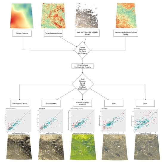
2.7. Model Development
- Soil organic carbon,
- Total nitrogen,
- Cation exchange capacity,
- Electrical conductivity,
- Inorganic carbon,
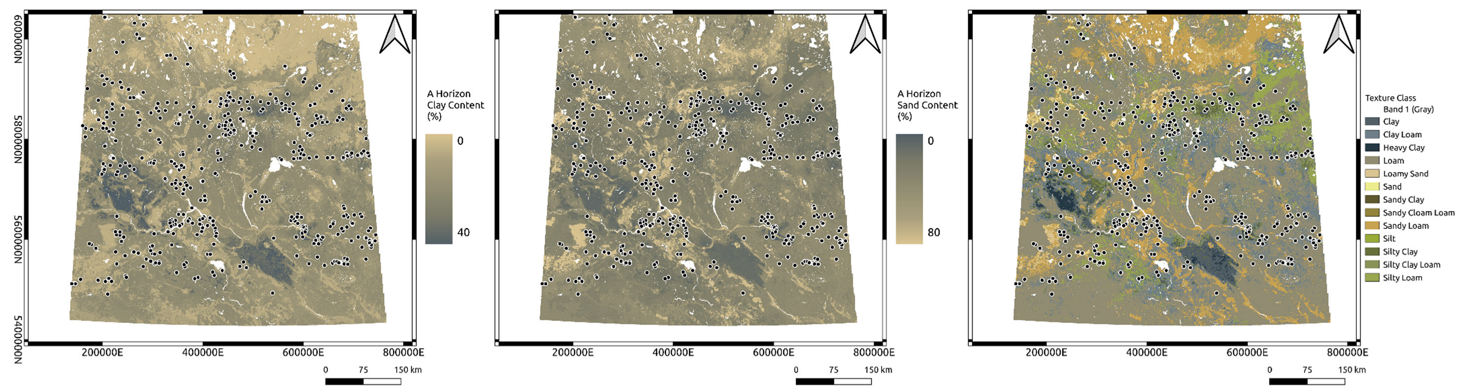
- Sand content,
- Clay content,
- Horizon thickness,
- Soil organic carbon stock
2.8. Model Validation
3. Results
4. Discussion
5. Conclusions
Supplementary Materials
Author Contributions
Funding
Data Availability Statement
Conflicts of Interest
References
- Bedard-Haughn, A.; Van Rees, K.; Bentham, M.; Krug, P.; Kiss, J.; Walters, K.; Heung, B.; Jamsrandorj, T.; Deters, R.; Cerkowniak, D.; et al. Saskatchewan Soil Information System (SKSIS) The Launch! Available online: https://harvest.usask.ca/bitstream/handle/10388/8664/A.Bedard-Haughn%20et%20al.2018.pdf?sequence=1 (accessed on 3 February 2021).
- Carré, F.; McBratney, A.B.; Mayr, T.; Montanarella, L. Digital Soil Assessments: Beyond DSM. Geoderma 2007, 142, 69–79. [Google Scholar] [CrossRef]
- McBratney, A.B.; Mendonça Santos, M.L.; Minasny, B. On Digital Soil Mapping. Geoderma 2003, 117, 3–52. [Google Scholar] [CrossRef]
- Gorelick, N.; Hancher, M.; Dixon, M.; Ilyushchenko, S.; Thau, D.; Moore, R. Google Earth Engine: Planetary-Scale Geospatial Analysis for Everyone. Remote Sens. Environ. 2017, 202, 18–27. [Google Scholar] [CrossRef]
- Maynard, J.J.; Levi, M.R. Hyper-Temporal Remote Sensing for Digital Soil Mapping: Characterizing Soil-Vegetation Response to Climatic Variability. Geoderma 2017, 285, 94–109. [Google Scholar] [CrossRef] [Green Version]
- Guo, L.; Fu, P.; Shi, T.; Chen, Y.; Zhang, H.; Meng, R.; Wang, S. Mapping Field-Scale Soil Organic Carbon with Unmanned Aircraft System-Acquired Time Series Multispectral Images. Soil Tillage Res. 2020, 196, 104477. [Google Scholar] [CrossRef]
- Fathololoumi, S.; Vaezi, A.R.; Alavipanah, S.K.; Ghorbani, A.; Saurette, D.; Biswas, A. Improved Digital Soil Mapping with Multitemporal Remotely Sensed Satellite Data Fusion: A Case Study in Iran. Sci. Total Environ. 2020, 721, 137703. [Google Scholar] [CrossRef]
- Demattê, J.A.M.; Fongaro, C.T.; Rizzo, R.; Safanelli, J.L. Geospatial Soil Sensing System (GEOS3): A Powerful Data Mining Procedure to Retrieve Soil Spectral Reflectance from Satellite Images. Remote Sens. Environ. 2018, 212, 161–175. [Google Scholar] [CrossRef]
- Bartholomeus, H.; Epema, G.; Schaepman, M. Determining Iron Content in Mediterranean Soils in Partly Vegetated Areas, Using Spectral Reflectance and Imaging Spectroscopy. Int. J. Appl. Earth Obs. Geoinf. 2007, 9, 194–203. [Google Scholar] [CrossRef] [Green Version]
- Bartholomeus, H.M.M.; Schaepman, M.E.E.; Kooistra, L.; Stevens, A.; Hoogmoed, W.B.B.; Spaargaren, O.S.P. Spectral Reflectance Based Indices for Soil Organic Carbon Quantification. Geoderma 2008, 145, 28–36. [Google Scholar] [CrossRef]
- Statistics Canada. 2016 Census of Agriculture. Available online: https://www.statcan.gc.ca/eng/ca2016 (accessed on 27 August 2020).
- Sorenson, P.T.; Shirtliffe, S.J.; Bedard-Haughn, A.K. Predictive Soil Mapping Using Historic Bare Soil Composite Imagery and Legacy Soil Survey Data. Geoderma 2021, 401, 115316. [Google Scholar] [CrossRef]
- Rogge, D.; Bauer, A.; Zeidler, J.; Mueller, A.; Esch, T.; Heiden, U. Building an Exposed Soil Composite Processor (SCMaP) for Mapping Spatial and Temporal Characteristics of Soils with Landsat Imagery (1984–2014). Remote Sens. Environ. 2018, 205, 1–17. [Google Scholar] [CrossRef] [Green Version]
- Safanelli, J.L.; Chabrillat, S.; Ben-Dor, E.; Demattê, J.A.M. Multispectral Models from Bare Soil Composites for Mapping Topsoil Properties over Europe. Remote Sens. 2020, 12, 1369. [Google Scholar] [CrossRef]
- Demattê, J.A.M.; Safanelli, J.L.; Poppiel, R.R.; Rizzo, R.; Silvero, N.E.Q.; de Sousa Mendes, W.; Bonfatti, B.R.; Dotto, A.C.; Salazar, D.F.U.; Alcântara de Oliveira Mello, F.; et al. Bare Earth’s Surface Spectra as a Proxy for Soil Resource Monitoring. Sci. Rep. 2020, 10, 4461. [Google Scholar] [CrossRef] [Green Version]
- Hengl, T.; Macmillan, R.A. Predictive Soil Mapping with R; Open Geo Hub Foundation: Wageningen, The Netherlands, 2019; ISBN 978-0-359-30635-0. [Google Scholar]
- Hengl, T.; Mendes de Jesus, J.; Heuvelink, G.B.M.; Ruiperez Gonzalez, M.; Kilibarda, M.; Blagotić, A.; Shangguan, W.; Wright, M.N.; Geng, X.; Bauer-Marschallinger, B.; et al. SoilGrids250m: Global Gridded Soil Information Based on Machine Learning. PLoS ONE 2017, 12, e0169748. [Google Scholar] [CrossRef] [Green Version]
- Sanderman, J.; Hengl, T.; Fiske, G.; Solvik, K.; Adame, M.F.; Benson, L.; Bukoski, J.J.; Carnell, P.; Cifuentes-Jara, M.; Donato, D.; et al. A Global Map of Mangrove Forest Soil Carbon at 30 m Spatial Resolution. Environ. Res. Lett. 2018, 13, 055022. [Google Scholar] [CrossRef]
- Viscarra Rossel, R.A.; Chen, C.; Grundy, M.J.; Searle, R.; Clifford, D.; Campbell, P.H. The Australian Three-Dimensional Soil Grid: Australia’s Contribution to the GlobalSoilMap Project. Soil Res. 2015, 53, 845. [Google Scholar] [CrossRef] [Green Version]
- Sothe, C.; Gonsamo, A.; Arabian, J.; Snider, J. Large Scale Mapping of Soil Organic Carbon Concentration with 3D Machine Learning and Satellite Observations. Geoderma 2022, 405, 115402. [Google Scholar] [CrossRef]
- Agriculture and Agri-Food Canada. Annual Crop Inventory. Available online: https://open.canada.ca/data/en/dataset/ba2645d5-4458-414d-b196-6303ac06c1c9 (accessed on 31 January 2021).
- Agriculture and Agri-Food Canada. National Pedon Database. Available online: https://open.canada.ca/data/en/dataset/6457fad6-b6f5-47a3-9bd1-ad14aea4b9e0 (accessed on 16 February 2021).
- Soil Classification Working Group the Canadian System of Soil Classification. The Canadian System of Soil Classification, 3rd ed.; Agriculture and Agri-Food Canada: Ottawa, ON, Canada, 1998; Volume 187. [Google Scholar]
- IUSS Working Group WRB. World Reference Base for Soil Resources 2014: International Soil Classification System for Naming Soils and Creating Legends for Soil Maps; Food and Agriculture Organization of the United Nations (FAO): Rome, Italy, 2014; ISBN 9789251083697. [Google Scholar]
- Baillie, I.C. Soil Survey Staff 1999, Soil Taxonomy: A Basic System of Soil Classification for Making and Interpreting Soil Surveys; Agricultural Handbook 436; Natural Resources Conservation Service (USDA): Washington, DC, USA, 1999. [Google Scholar]
- Wright, M.N.; Ziegler, A. Ranger: A Fast Implementation of Random Forests for High Dimensional Data in C++ and R. J. Stat. Softw. 2017, 77, 1–17. [Google Scholar] [CrossRef] [Green Version]
- Gitelson, A.A.; Merzlyak, M.N.; Chivkunova, O.B. Optical Properties and Nondestructive Estimation of Anthocyanin Content in Plant Leaves. Photochem. Photobiol. 2001, 74, 38. [Google Scholar] [CrossRef]
- Scudiero, E.; Skaggs, T.H.; Corwin, D.L. Regional-Scale Soil Salinity Assessment Using Landsat ETM + Canopy Reflectance. Remote Sens. Environ. 2015, 169, 335–343. [Google Scholar] [CrossRef]
- Sorenson, P. Google Earth Engine Scripts for Generating Predictive Soil Mapping Environmental Covariates. Available online: https://github.com/prestonsorenson/Google_Earth_Engine_PSM/tree/main (accessed on 16 August 2021).
- Copernicus Climate Change Service (C3S). ERA5: Fifth Generation of ECMWF Atmospheric Reanalyses of the Global Climate. Available online: https://cds.climate.copernicus.eu/cdsapp#!/home (accessed on 14 October 2021).
- Du, Y.; Zhang, Y.; Ling, F.; Wang, Q.; Li, W.; Li, X. Water Bodies’ Mapping from Sentinel-2 Imagery with Modified Normalized Difference Water Index at 10-m Spatial Resolution Produced by Sharpening the SWIR Band. Remote Sens. 2016, 8, 354. [Google Scholar] [CrossRef] [Green Version]
- Kokaly, R.F.; Clark, R.N.; Swayze, G.A.; Livo, K.E.; Hoefen, T.M.; Pearson, N.C.; Wise, R.A.; Benzel, W.M.; Lowers, H.A.; Driscoll, R.L.; et al. USGS Spectral Library Version 7; United States Geological Survey (USGS): Reston, VA, USA, 2017; Volume 7. [Google Scholar]
- Sorenson, P. Landsat 5 Bare Soil Composite Script. Available online: https://github.com/prestonsorenson/GEE_Bare_Soil_Composite/blob/main/Bare_Soil_Composite_Landsat_5 (accessed on 30 April 2021).
- Japan Aerospace Exploration Agency. ALOS Global Digital Surface Model. Available online: https://www.eorc.jaxa.jp/ALOS/en/aw3d30/index.htm (accessed on 24 September 2021).
- Boehner, J.; Selige, T. Spatial Prediction of Soil Attributes Using Terrain Analysis and Climate Regionalisation. In SAGA—Analyses and Modelling Applications; Boehner, J., McCloy, K.R., Strobl, J., Eds.; Göttinger Geographische Abhandlungen; Geographical Institute of the University of Göttingen: Göttingen, Germany, 2006; pp. 13–27. [Google Scholar]
- Kiss, J. Predictive Mapping of Wetland Types and Associated Soils through Digital Elevation Model Analyses in the Canadian Prairie Pothole Region. M.Sc. Thesis, University of Saskatchewan, Saskatoon, SK, Canada, 2018. [Google Scholar]
- Roudier, P. Clhs: A R Package for Conditioned Latin Hypercube Sampling 2011. Available online: https://github.com/pierreroudier/clhs/(accessed on 14 November 2021).
- Biswas, A.; Zhang, Y. Sampling Designs for Validating Digital Soil Maps: A Review. Pedosphere 2018, 28, 1–15. [Google Scholar] [CrossRef]
- Sorenson, P. Predictive Soil Mapping Scripts. Available online: https://github.com/prestonsorenson/Predictive_Soil_Mapping (accessed on 28 October 2021).
- Kasraei, B.; Heung, B.; Saurette, D.D.; Schmidt, M.G.; Bulmer, C.E.; Bethel, W. Quantile Regression as a Generic Approach for Estimating Uncertainty of Digital Soil Maps Produced from Machine-Learning. Environ. Model. Softw. 2021, 144, 105139. [Google Scholar] [CrossRef]
- Vaysse, K.; Lagacherie, P. Evaluating Digital Soil Mapping Approaches for Mapping GlobalSoilMap Soil Properties from Legacy Data in Languedoc-Roussillon (France). Geoderma Reg. 2015, 4, 20–30. [Google Scholar] [CrossRef]
- Rizzo, R.; Medeiros, L.G.; de Mello, D.C.; Marques, K.P.P.; de Mendes, W.S.; Quiñonez Silvero, N.E.; Dotto, A.C.; Bonfatti, B.R.; Demattê, J.A.M. Multi-Temporal Bare Surface Image Associated with Transfer Functions to Support Soil Classification and Mapping in Southeastern Brazil. Geoderma 2020, 361, 114018. [Google Scholar] [CrossRef]
- Wang, S.; Zhuang, Q.; Wang, Q.; Jin, X.; Han, C. Mapping Stocks of Soil Organic Carbon and Soil Total Nitrogen in Liaoning Province of China. Geoderma 2017, 305, 250–263. [Google Scholar] [CrossRef]
- Wang, B.; Waters, C.; Orgill, S.; Gray, J.; Cowie, A.; Clark, A.; Liu, D.L. High Resolution Mapping of Soil Organic Carbon Stocks Using Remote Sensing Variables in the Semi-Arid Rangelands of Eastern Australia. Sci. Total Environ. 2018, 630, 367–378. [Google Scholar] [CrossRef]
- Liddicoat, C.; Maschmedt, D.; Clifford, D.; Searle, R.; Herrmann, T.; MacDonald, L.M.; Baldock, J. Predictive Mapping of Soil Organic Carbon Stocks in South Australia’s Agricultural Zone. Soil Res. 2015, 53, 956–973. [Google Scholar] [CrossRef]
- Nussbaum, M.; Spiess, K.; Baltensweiler, A.; Grob, U.; Keller, A.; Greiner, L.; Schaepman, M.E.; Papritz, A. Evaluation of Digital Soil Mapping Approaches with Large Sets of Environmental Covariates. Soil 2018, 4, 1–22. [Google Scholar] [CrossRef] [Green Version]
- Poppiel, R.R.; Demattê, J.A.M.; Rosin, N.A.; Campos, L.R.; Tayebi, M.; Bonfatti, B.R.; Ayoubi, S.; Tajik, S.; Afshar, F.A.; Jafari, A.; et al. High Resolution Middle Eastern Soil Attributes Mapping via Open Data and Cloud Computing. Geoderma 2021, 385, 114890. [Google Scholar] [CrossRef]
- Rossel, R.A.V.; Behrens, T.; Viscarra Rossel, R.A.; Behrens, T. Using Data Mining to Model and Interpret Soil Diffuse Reflectance Spectra. Geoderma 2010, 158, 46–54. [Google Scholar] [CrossRef]
- Nabiollahi, K.; Taghizadeh-Mehrjardi, R.; Shahabi, A.; Heung, B.; Amirian-Chakan, A.; Davari, M.; Scholten, T. Assessing Agricultural Salt-Affected Land Using Digital Soil Mapping and Hybridized Random Forests. Geoderma 2021, 385, 114858. [Google Scholar] [CrossRef]
- Taghizadeh-Mehrjardi, R.; Schmidt, K.; Toomanian, N.; Heung, B.; Behrens, T.; Mosavi, A.; Band, S.; Amirian-Chakan, A.; Fathabadi, A.; Scholten, T. Improving the Spatial Prediction of Soil Salinity in Arid Regions Using Wavelet Transformation and Support Vector Regression Models. Geoderma 2021, 383, 114793. [Google Scholar] [CrossRef]
- Ma, G.; Ding, J.; Han, L.; Zhang, Z.; Ran, S. Digital Mapping of Soil Salinization Based on Sentinel-1 and Sentinel-2 Data Combined with Machine Learning Algorithms. Reg. Sustain. 2021, 2, 177–188. [Google Scholar] [CrossRef]
- Kiss, J.; Bedard-Haughn, A. Predictive Mapping of Solute-rich Wetlands in the Canadian Prairie Pothole Region Through High-resolution Digital Elevation Model Analyses. Wetlands 2021, 41, 38. [Google Scholar] [CrossRef]
- Jenny, H. Factors of Soil Formation. Soil Sci. 1941, 52, 415. [Google Scholar] [CrossRef]
- Becker, W.R.; Ló, T.B.; Johann, J.A.; Mercante, E. Statistical Features for Land Use and Land Cover Classification in Google Earth Engine. Remote Sens. Appl. 2021, 21, 100459. [Google Scholar] [CrossRef]
- Gilabert, M.A.; González-Piqueras, J.; García-Haro, F.J.; Meliá, J. A Generalized Soil-Adjusted Vegetation Index. Remote Sens. Environ. 2002, 82, 303–310. [Google Scholar] [CrossRef]
- Miao, Y.; Mulla, D.J.; Robert, P.C. Identifying Important Factors Influencing Corn Yield and Grain Quality Variability Using Artificial Neural Networks. Precis. Agric. 2006, 7, 117–135. [Google Scholar] [CrossRef]
- He, Y.; Wei, Y.; DePauw, R.; Qian, B.; Lemke, R.; Singh, A.; Cuthbert, R.; McConkey, B.; Wang, H. Spring Wheat Yield in the Semiarid Canadian Prairies: Effects of Precipitation Timing and Soil Texture over Recent 30 Years. Field Crops Res. 2013, 149, 329–337. [Google Scholar] [CrossRef]


| Canadian System of Soil Science Classification | World Reference Base | United States Department of Agriculture Soil Classification System | n |
|---|---|---|---|
| Brunisol | Cambisol | Inceptisol | 3 |
| Chernozem | Kastanozem, Chernozem, Greyzem, Phaeozem | Borolls | 398 |
| Gleysol | Gleysol | Aqu suborders | 7 |
| Luvisol | Luvisol | Boralfs, Udalfs | 66 |
| Regosol | Regosol | Entisol | 25 |
| Solonetz | Solonetz | Natric Great Groups | 73 |
| Vertisol | Vertisol | Haplocryerts | 5 |
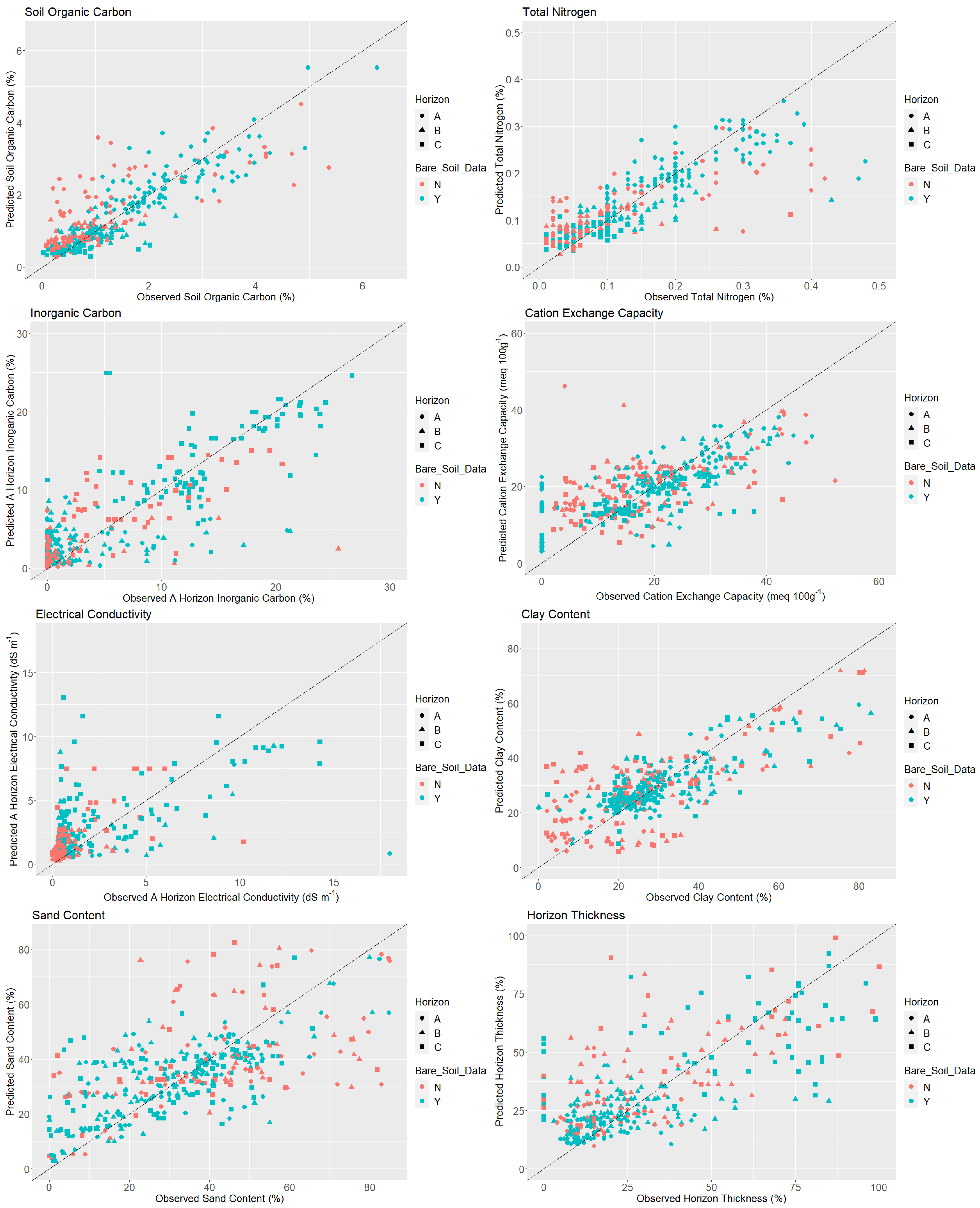
| Soil Property | Horizon | Null Model Root Mean Square Error | Predictive Model R2 | Predictive Model Root Mean Square Error | Predictive Model Concordance Correlation Coefficient | S |
|---|---|---|---|---|---|---|
| Soil Organic Carbon (%) | Overall | 1.14 | 0.71 | 0.61 | 0.83 | −0.07 |
| A | 1.39 | 0.49 | 0.85 | 0.64 | −0.11 | |
| B | 0.77 | 0.21 | 0.40 | 0.39 | −0.06 | |
| C | 1.09 | 0.11 | 0.31 | 0.25 | −0.01 | |
| Total Nitrogen (%) | Overall | 0.10 | 0.65 | 0.06 | 0.76 | 0.00 |
| A | 0.12 | 0.48 | 0.07 | 0.60 | 0.01 | |
| B | 0.07 | 0.25 | 0.05 | 0.39 | 0.00 | |
| C | 0.09 | 0.36 | 0.04 | 0.44 | 0.00 | |
| Inorganic Carbon (%) | Overall | 8.09 | 0.65 | 4.79 | 0.79 | −0.25 |
| A | 5.66 | 0.11 | 3.07 | 0.29 | −0.75 | |
| B | 7.08 | 0.16 | 5.67 | 0.25 | −0.10 | |
| C | 10.88 | 0.56 | 5.42 | 0.73 | 0.18 | |
| Electrical Conductivity (dS m−1) | Overall | 2.50 | 0.36 | 2.18 | 0.57 | −0.61 |
| A | 1.94 | 0.08 | 1.67 | 0.23 | −0.28 | |
| B | 1.94 | 0.26 | 1.67 | 0.47 | −0.50 | |
| C | 3.40 | 0.34 | 3.00 | 0.53 | −1.09 | |
| Cation Exchange Capacity (meq 100 g−1) | Overall | 11.27 | 0.46 | 8.18 | 0.63 | −0.42 |
| A | 12.09 | 0.47 | 8.80 | 0.63 | −0.61 | |
| B | 10.12 | 0.41 | 7.81 | 0.61 | −0.22 | |
| C | 11.37 | 0.36 | 7.81 | 0.51 | −0.40 | |
| Clay (%) | Overall | 15.62 | 0.55 | 10.47 | 0.70 | −0.47 |
| A | 14.36 | 0.65 | 8.23 | 0.76 | −1.05 | |
| B | 15.77 | 0.50 | 11.10 | 0.67 | 0.43 | |
| C | 16.81 | 0.49 | 12.00 | 0.66 | −0.68 | |
| Sand (%) | Overall | 22.55 | 0.44 | 16.99 | 0.64 | −0.61 |
| A | 21.46 | 0.52 | 14.89 | 0.70 | 0.57 | |
| B | 22.45 | 0.44 | 17.03 | 0.64 | −1.84 | |
| C | 23.82 | 0.37 | 19.07 | 0.58 | −0.74 | |
| Horizon Thickness (%) | Overall | 0.55 | 0.76 | 0.27 | 0.86 | 0.00 |
| A | 0.38 | 0.06 | 0.10 | 0.21 | −0.03 | |
| B | 0.30 | 0.06 | 0.23 | 0.21 | −0.01 | |
| C | 0.80 | 0.66 | 0.39 | 0.79 | 0.03 | |
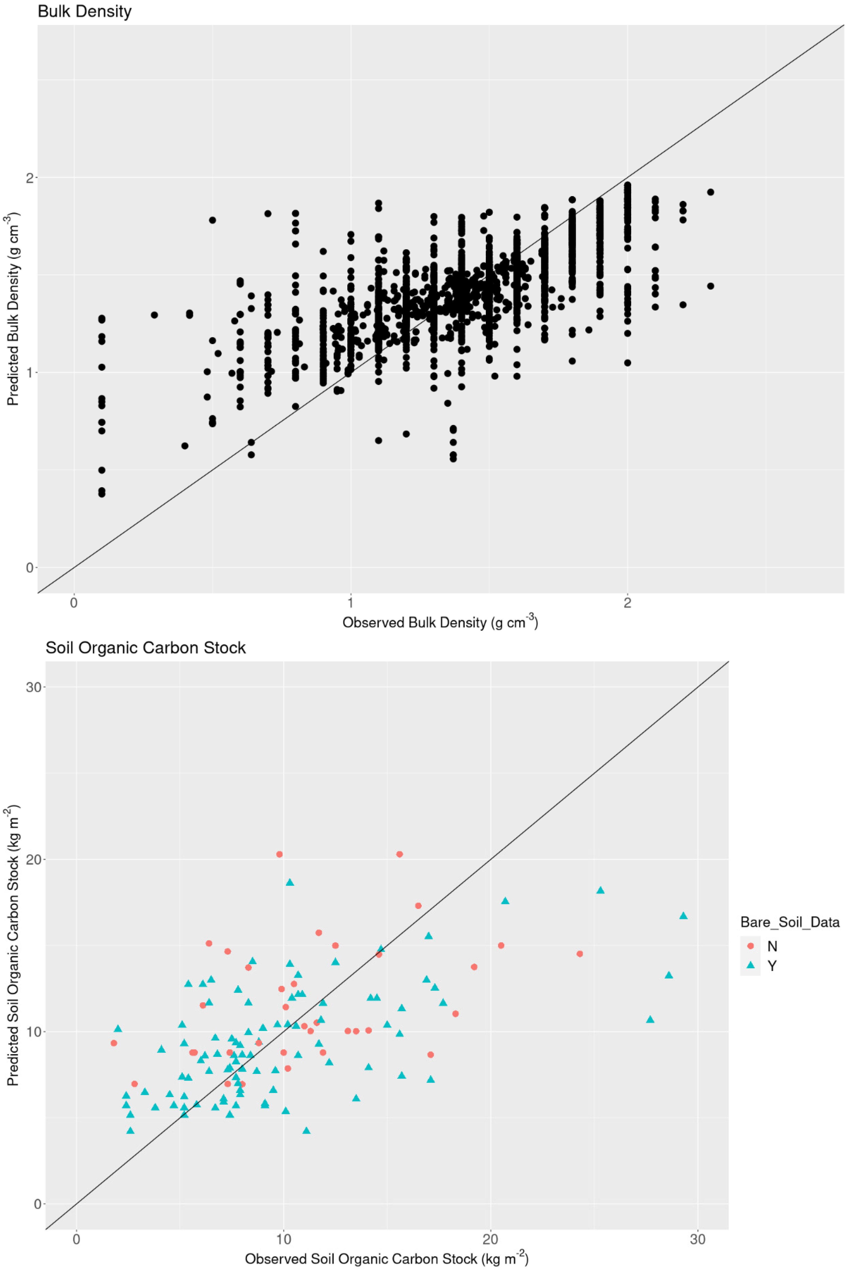
| Bulk Density (g cm−3) | Overall | 0.3 | 0.52 | 0.20 | 0.66 | <0.01 |
| Soil Organic Carbon Stock (kg m−2) | Overall | 5.83 | 0.27 | 4.84 | 0.47 | 0.31 |
| Soil Property | Features | Relative Feature Importance |
|---|---|---|
| Soil Organic Carbon (%) | Horizon | 0.46 |
| ARI No Bare Soil Pixels | 0.15 | |
| Standard Deviation of NDVI | 0.09 | |
| September and October NDVI | 0.08 | |
| Precipitation | 0.08 | |
| Temperature | 0.07 | |
| Bare Soil Band 7 | 0.07 | |
| Bulk Density (g cm−3) | Soil Organic Carbon | 0.26 |
| Sand Content | 0.26 | |
| Silt Content | 0.25 | |
| Clay Content | 0.24 | |
| Profile Soil Organic Carbon Stocks (kg m2) | Standard Deviation of NDVI | 0.18 |
| Precipitation | 0.14 | |
| Temperature | 0.14 | |
| September and October NDVI | 0.13 | |
| CRSI No Bare Soil Pixels | 0.12 | |
| CRSI | 0.12 | |
| Bare Soil Band 2 | 0.11 | |
| SAGA Wetness Index | 0.05 | |
| Total Nitrogen (%) | Horizon | 0.52 |
| Bare Soil Band 7 | 0.09 | |
| September and October NDVI | 0.08 | |
| Standard Deviation of NDVI | 0.08 | |
| Temperature | 0.08 | |
| Precipitation | 0.07 | |
| CRSI No Bare Soil Pixels | 0.07 | |
| Cation Exchange Capacity (meq 100 g−1) | Standard Deviation of NDVI | 0.17 |
| Bare Soil Band 5 | 0.17 | |
| Horizon | 0.17 | |
| July and August SAVI No Bare Soil Pixels | 0.16 | |
| Temperature | 0.14 | |
| Precipitation | 0.13 | |
| Standard Deviation of Elevation (101 × 101 focal window with 9 × 9 median focal filter of the input surface model) | 0.06 | |
| Electrical Conductivity (dS m−1) | Horizon | 0.18 |
| Temperature | 0.16 | |
| September and October NDVI | 0.15 | |
| CRSI | 0.14 | |
| Precipitation | 0.12 | |
| Bare Soil Band 5 | 0.12 | |
| Standard Deviation of Elevation (21 × 21 focal window with 3 × 3 median focal filter of the input surface model) | 0.07 | |
| Standard Deviation of Elevation (3 × 3 focal window with 3 × 3 median focal filter of the input surface model) | 0.06 | |
| Inorganic Carbon (%) | Horizon | 0.49 |
| Precipitation | 0.21 | |
| Temperature | 0.11 | |
| ARI No Bare Soil Pixels | 0.10 | |
| July and August NDVI | 0.09 | |
| Clay (%) | Bare Soil Band 5 | 0.20 |
| Standard Deviation of NDVI | 0.18 | |
| September and October NDVI | 0.17 | |
| Temperature | 0.13 | |
| Precipitation | 0.13 | |
| CRSI No Bare Soil Pixels | 0.13 | |
| Horizon | 0.05 | |
| Sand (%) | Standard Deviation of NDVI | 0.20 |
| September and October of NDVI | 0.17 | |
| Bare Soil Band 7 | 0.15 | |
| Temperature | 0.14 | |
| ARI No Bare Soil Pixels | 0.13 | |
| Precipitation | 0.06 | |
| Standardized Height | 0.06 | |
| Horizon | 0.02 | |
| Horizon Thickness | Horizon | 0.48 |
| Precipitation | 0.14 | |
| Temperature | 0.13 | |
| ARI | 0.07 | |
| Standard Deviation of NDVI | 0.07 | |
| Bare Soil Band 7 | 0.06 | |
| Standard Deviation of Elevation (3 × 3 focal window with 3 × 3 median focal filter of the input surface model) | 0.04 |
Publisher’s Note: MDPI stays neutral with regard to jurisdictional claims in published maps and institutional affiliations. |
© 2022 by the authors. Licensee MDPI, Basel, Switzerland. This article is an open access article distributed under the terms and conditions of the Creative Commons Attribution (CC BY) license (https://creativecommons.org/licenses/by/4.0/).
Share and Cite
Sorenson, P.T.; Kiss, J.; Bedard-Haughn, A.K.; Shirtliffe, S. Multi-Horizon Predictive Soil Mapping of Historical Soil Properties Using Remote Sensing Imagery. Remote Sens. 2022, 14, 5803. https://doi.org/10.3390/rs14225803
Sorenson PT, Kiss J, Bedard-Haughn AK, Shirtliffe S. Multi-Horizon Predictive Soil Mapping of Historical Soil Properties Using Remote Sensing Imagery. Remote Sensing. 2022; 14(22):5803. https://doi.org/10.3390/rs14225803
Chicago/Turabian StyleSorenson, Preston T., Jeremy Kiss, Angela K. Bedard-Haughn, and Steve Shirtliffe. 2022. "Multi-Horizon Predictive Soil Mapping of Historical Soil Properties Using Remote Sensing Imagery" Remote Sensing 14, no. 22: 5803. https://doi.org/10.3390/rs14225803