
Multi-Scale Validation and Uncertainty Analysis of GEOV3 and MuSyQ FVC Products: A Case Study of an Alpine Grassland Ecosystem

 ,
,
Abstract
:1. Introduction
2. Materials and Methods
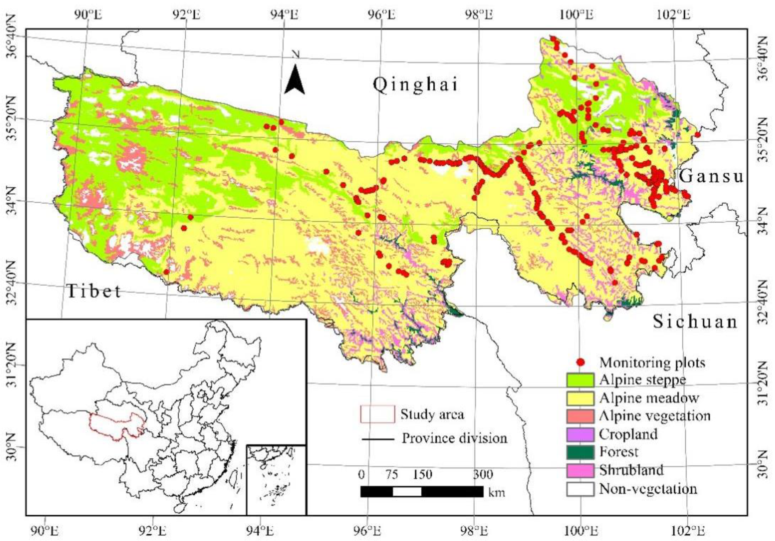
2.1. Study Area
2.2. Data Source and Pre-Processing
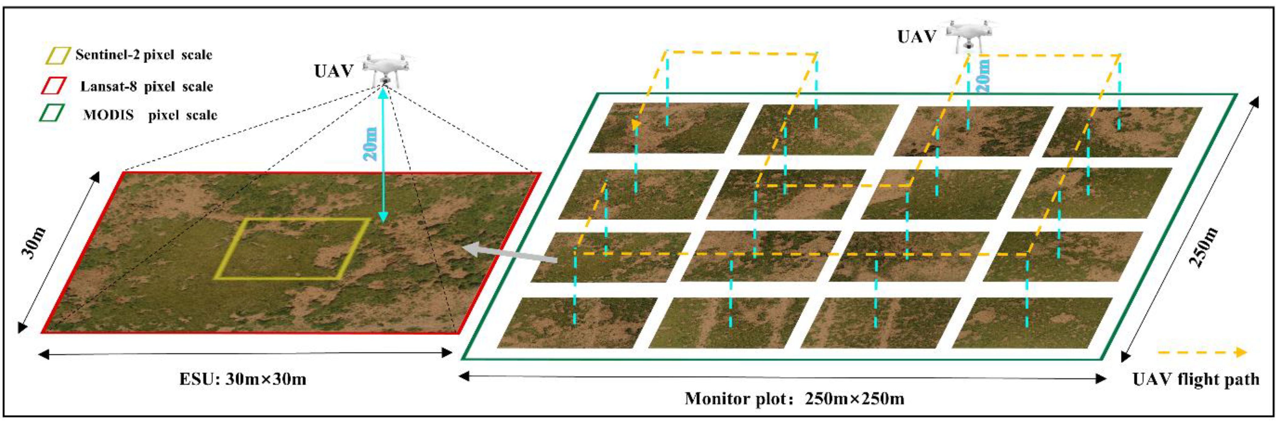
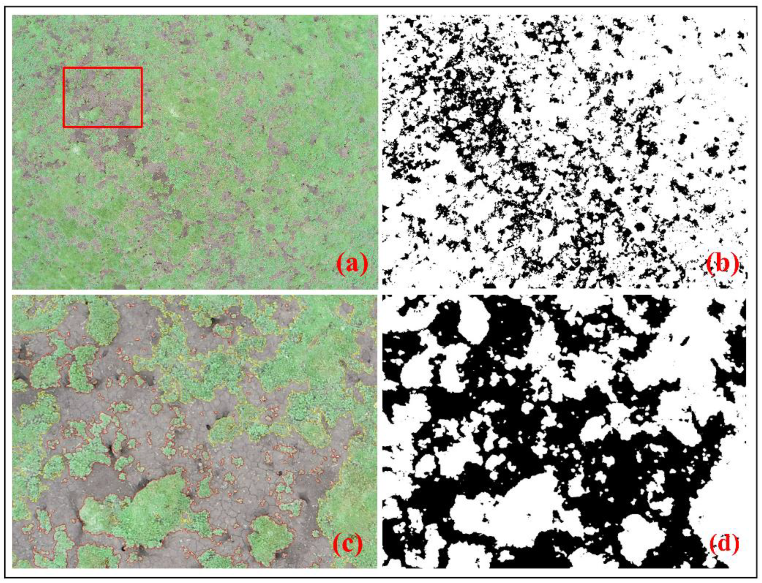
2.2.1. Field Data Based on UAV Imagery
2.2.2. Remote Sensing Data
Sentinel-2 Data
MODIS Data
2.2.3. FVC Product Data
MuSyQ FVC
GEOV3 FVC
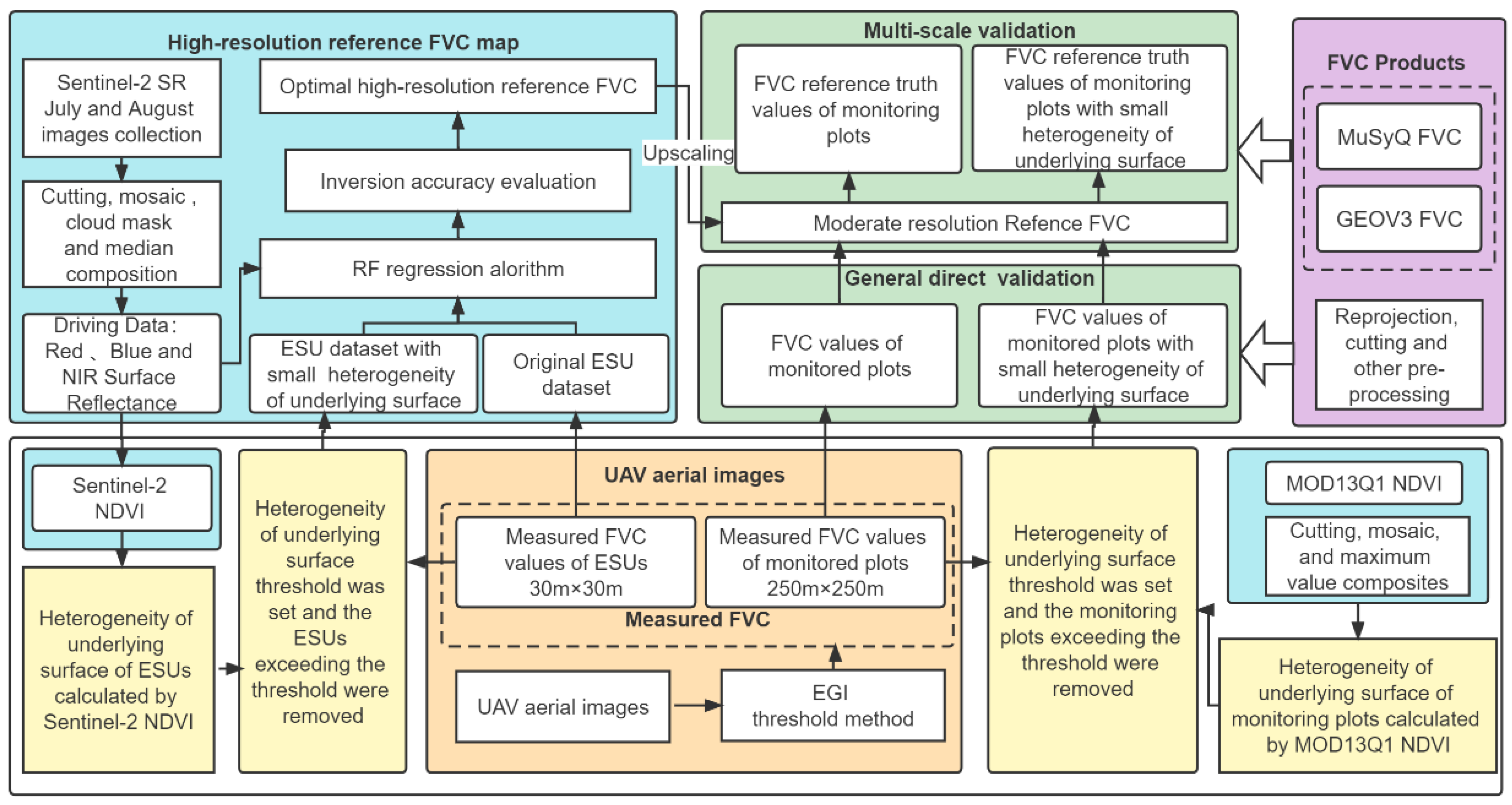
2.3. Methods
2.3.1. General Direct Validation Method
2.3.2. Multi-Scale Validation Method
2.3.3. Method of Evaluating the HUS of the Monitoring Plots and Surrounding Area
2.3.4. High-Resolution Reference FVC Data Inversion Method
2.3.5. Accuracy Assessment
3. Results
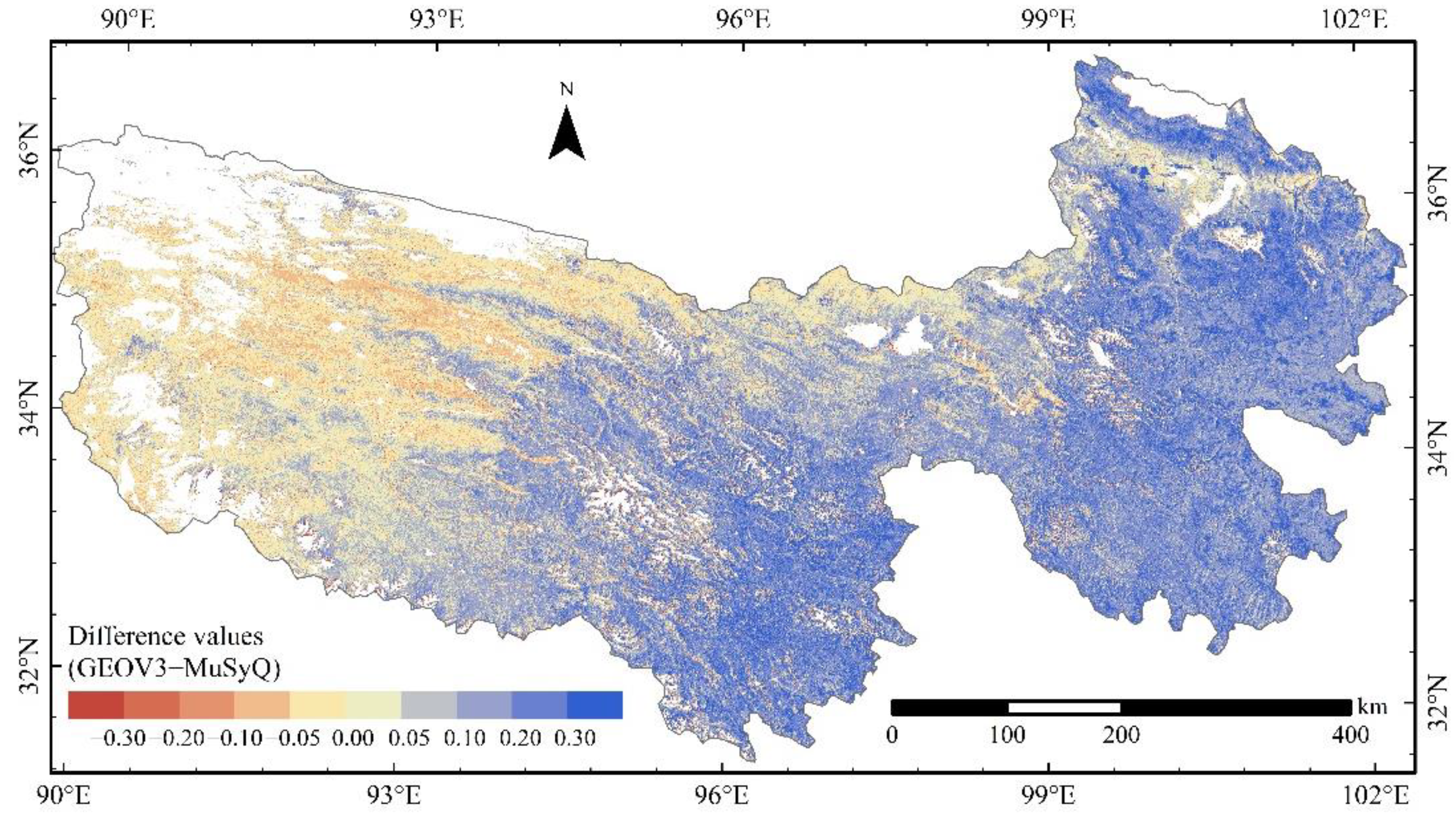
3.1. Comparison of GEOV3 and MuSyQ FVC
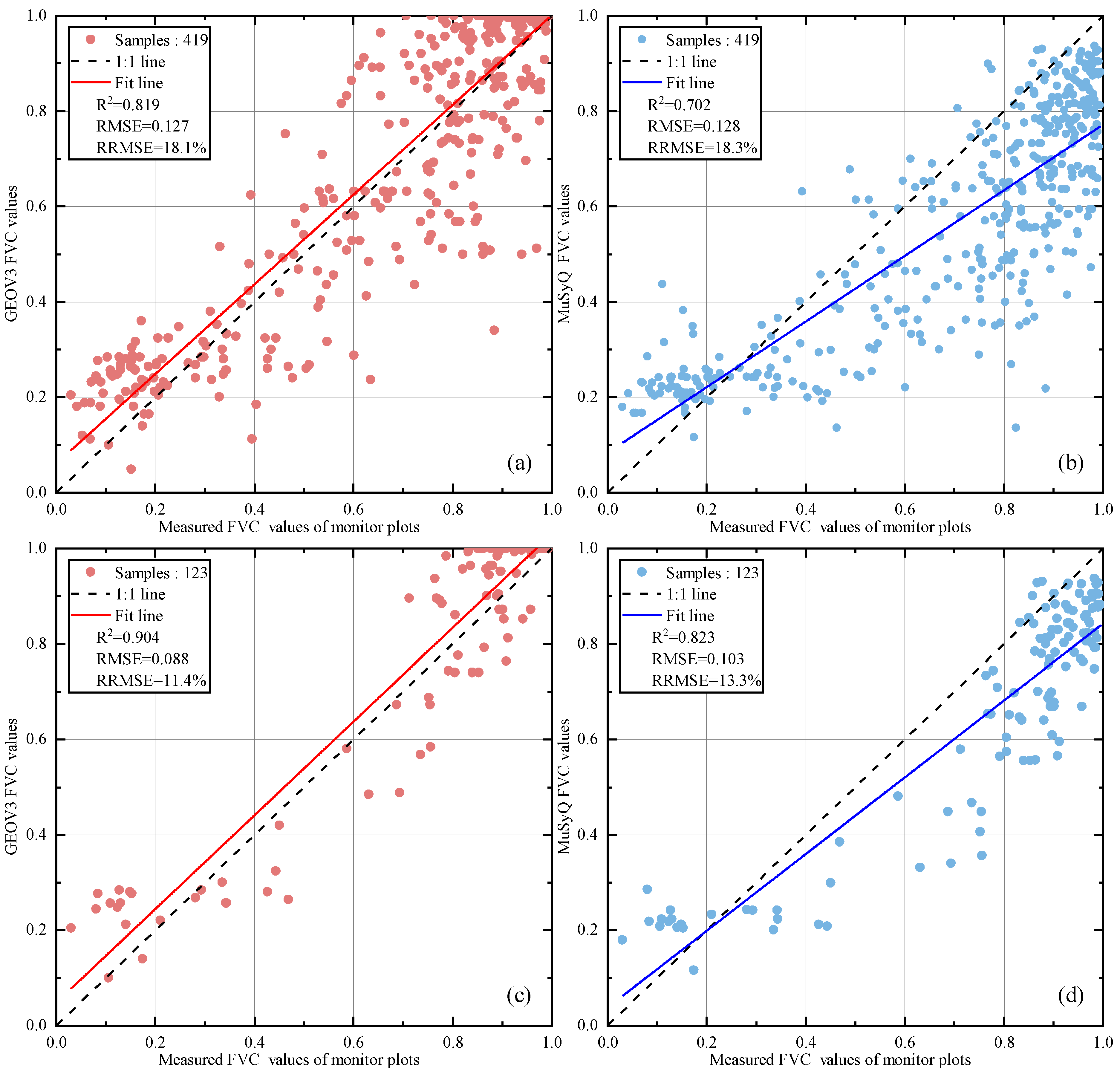
3.2. Direct Validation of GEOV3 and MuSyQ FVC Products Based on the Measured Values of Remote Sensing Monitoring Plots
3.3. Validation of GEOV3 and MuSyQ FVC Products with Using the Multi-Scale Validation
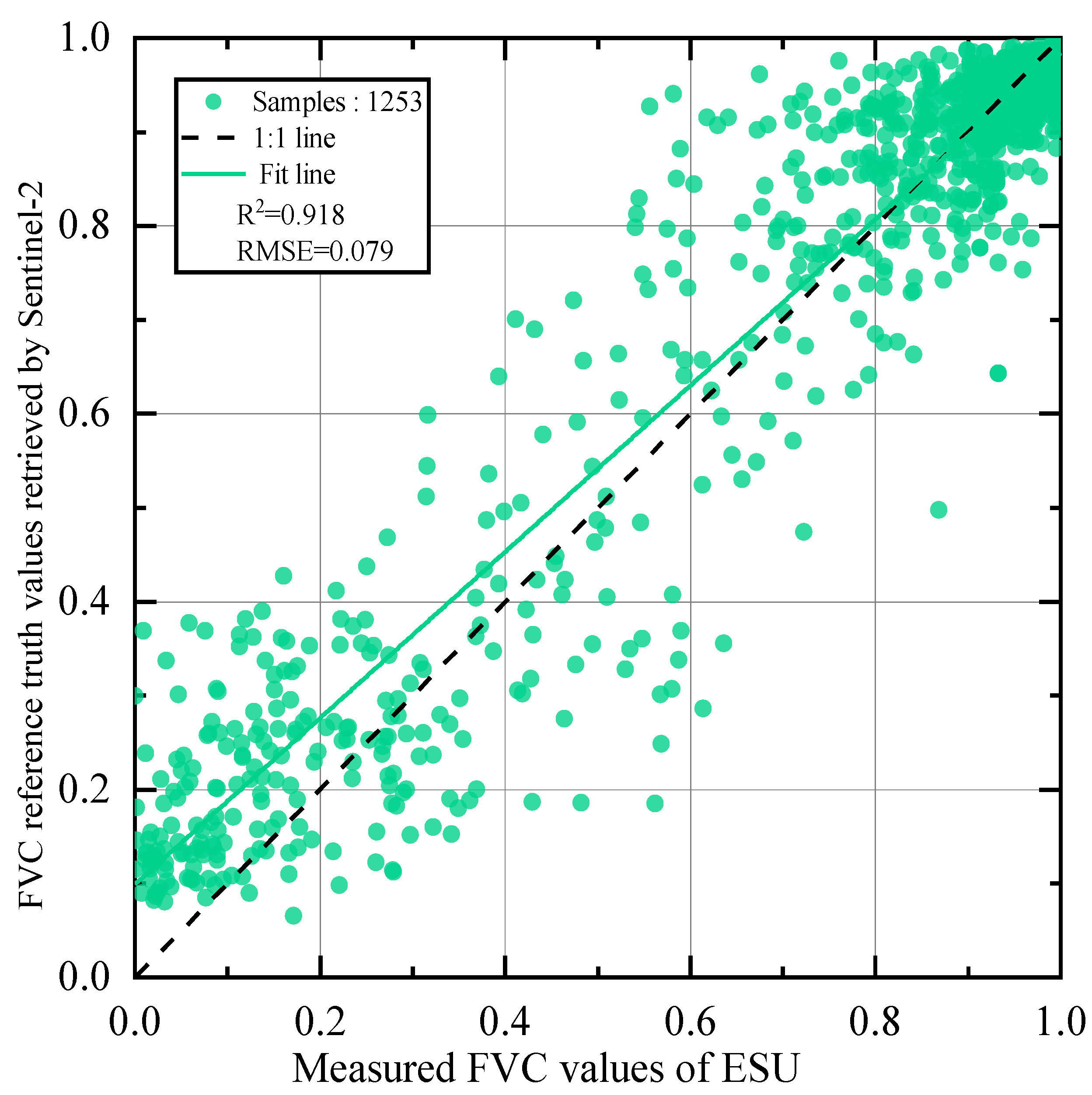
3.3.1. Inversion of High-Resolution FVC
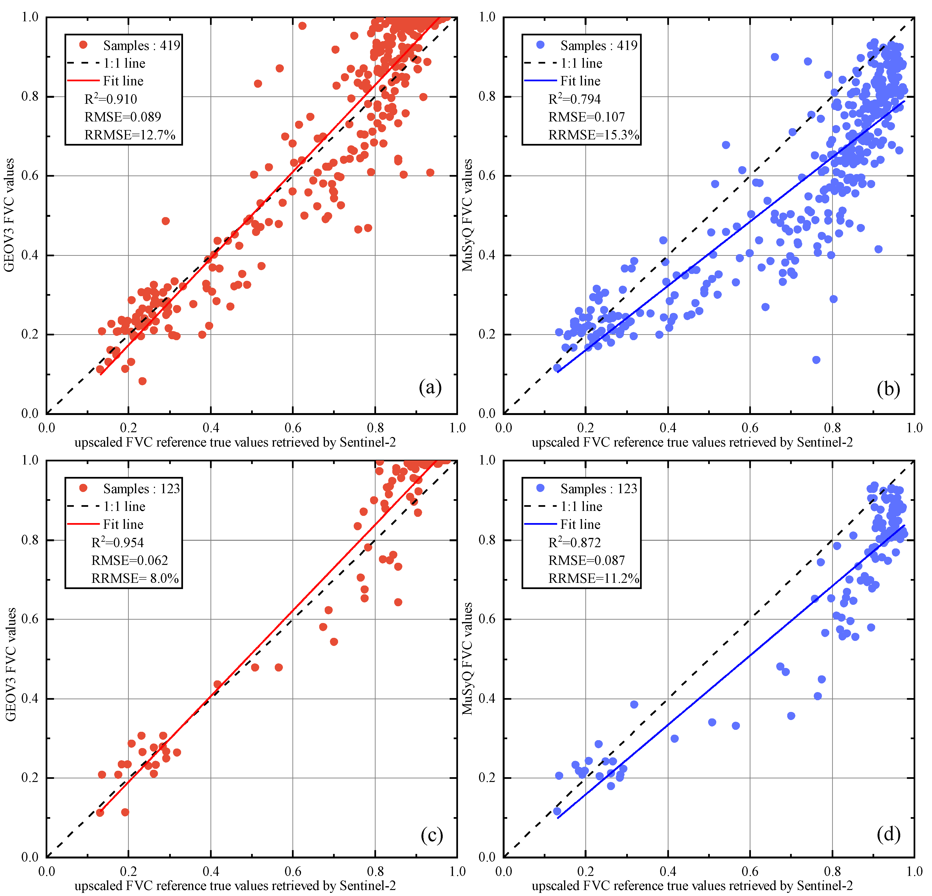
3.3.2. GEOV3 and MuSyQ FVC Validation Using a High-Resolution FVC Map
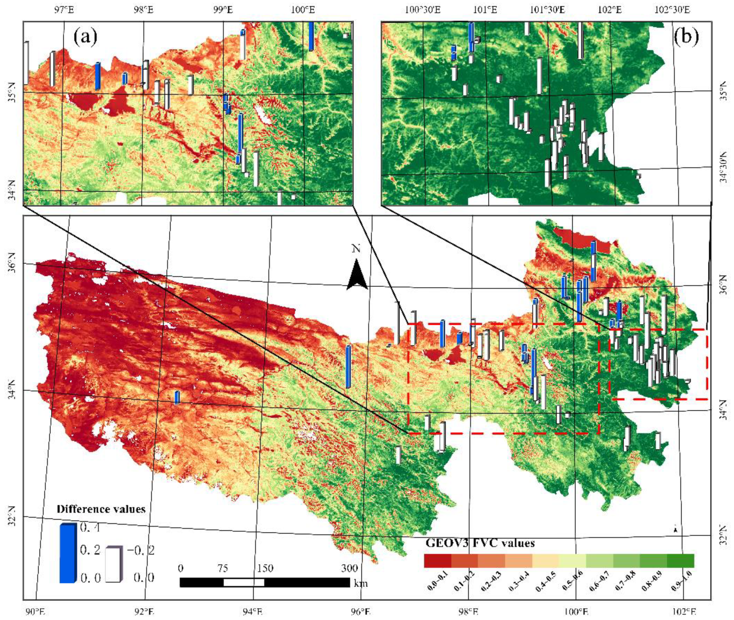
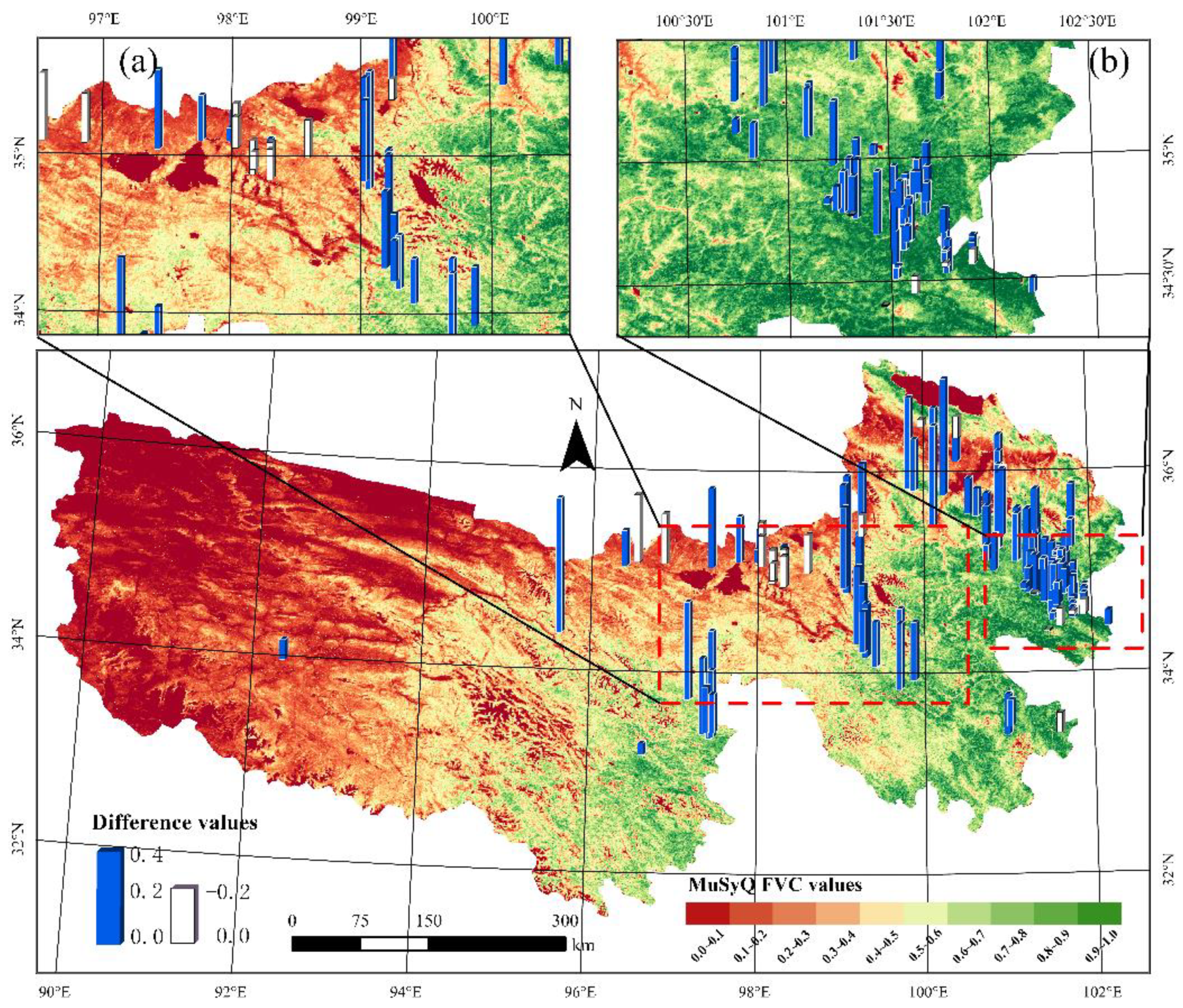
3.4. Error Distribution Pattern of GEOV3 and MuSyQ FVC Products
4. Discussion
4.1. Comparative Analysis of the Differences between the GEOV3 and MuSyQ FVC Products
4.2. Assessment of the Uncertainty of the Direct Validation Method
4.3. Assessment of Uncertainty of Multi-Scale Validation Method Based on High-Resolution Data
4.4. Error Analysis of GEOV3 and MuSyQ FVC Products
5. Conclusions
Author Contributions
Funding
Data Availability Statement
Acknowledgments
Conflicts of Interest
References
- Baret, F.; Weiss, M.; Lacaze, R.; Camacho, F.; Makhmara, H.; Pacholcyzk, P.; Smets, B. GEOV1: LAI and FAPAR Essential Climate Variables and FCOVER Global Time Series Capitalizing over Existing Products. Part1: Principles of Development and Production. Remote Sens. Environ. 2013, 137, 299–309. [Google Scholar] [CrossRef]
- Jia, K.; Yang, L.; Liang, S.; Xiao, Z.; Zhao, X.; Yao, Y.; Zhang, X.; Jiang, B.; Liu, D. Long-Term Global Land Surface Satellite (GLASS) Fractional Vegetation Cover Product Derived from MODIS and AVHRR Data. IEEE J. Sel. Top. Appl. Earth Obs. Remote Sens. 2019, 12, 508–518. [Google Scholar] [CrossRef]
- Gitelson, A.A.; Kaufman, Y.J.; Stark, R.; Rundquist, D. Novel Algorithms for Remote Estimation of Vegetation Fraction. Remote Sens. Environ. 2002, 80, 76–87. [Google Scholar] [CrossRef] [Green Version]
- Yang, Y.; Chen, J.; Huang, R.; Feng, Z.; Zhou, G.; You, H.; Han, X. Construction of Ecological Security Pattern Based on the Importance of Ecological Protection—A Case Study of Guangxi, a Karst Region in China. Int. J. Environ. Res. Public Health 2022, 19, 5699. [Google Scholar] [CrossRef] [PubMed]
- Liu, D.; Jia, K.; Wei, X.; Xia, M.; Zhang, X.; Yao, Y.; Zhang, X.; Wang, B. Spatiotemporal Comparison and Validation of Three Global-Scale Fractional Vegetation Cover Products. Remote Sens. 2019, 11, 2524. [Google Scholar] [CrossRef] [Green Version]
- Yang, L.; Jia, K.; Liang, S.; Liu, J.; Wang, X. Comparison of Four Machine Learning Methods for Generating the Glass Fractional Vegetation Cover Product from Modis Data. Remote Sens. 2016, 8, 382. [Google Scholar] [CrossRef] [Green Version]
- Zhou, G. Urban High-Resolution Remote Sensing: Algorithms and Modeling; CRC Press: Boca Raton, FL, USA, 2020; ISBN 1003082432. [Google Scholar]
- Roujean, J.L.; Lacaze, R. Global Mapping of Vegetation Parameters from POLDER Multiangular Measurements for Studies of Surface-Atmosphere Interactions: A Pragmatic Method and Its Validation. J. Geophys. Res. Atmos. 2002, 107, ACL 6-1–ACL 6-14. [Google Scholar] [CrossRef]
- García-Haro, J.; Camacho de Coca, F.; Meliá, J.; Martinez, B. Operational Derivation of Vegetation Products in the Framework of the LSA SAF Project. In Proceedings of the 2005 EUMETSAT Meteorological Satellite Conference, Dubrovnik, Croatia, 19–23 September 2005. [Google Scholar]
- Baret, F.; Pavageau, K.; Béal, D.; Weiss, M.; Berthelot, B.; Regner, P. Algorithm Theoretical Basis Document for MERIS Top of Atmosphere Land Products (TOA_VEG); INRA-CSE: Avignon, France, 2006. [Google Scholar]
- Baret, F.; Hagolle, O.; Geiger, B.; Bicheron, P.; Miras, B.; Huc, M.; Berthelot, B.; Niño, F.; Weiss, M.; Samain, O.; et al. LAI, FAPAR and FCover CYCLOPES Global Products Derived from VEGETATION. Part 1: Principles of the Algorithm. Remote Sens. Environ. 2007, 110, 275–286. [Google Scholar] [CrossRef] [Green Version]
- Zhao, J.; Li, J.; Liu, Q.; Xu, B.; Yu, W.; Lin, S.; Hu, Z. Estimating Fractional Vegetation Cover from Leaf Area Index and Clumping Index Based on the Gap Probability Theory. Int. J. Appl. Earth Obs. Geoinf. 2020, 90, 102112. [Google Scholar] [CrossRef]
- Camacho, F.; Cernicharo, J.; Lacaze, R.; Baret, F.; Weiss, M. GEOV1: LAI, FAPAR Essential Climate Variables and FCOVER Global Time Series Capitalizing over Existing Products. Part 2: Validation and Intercomparison with Reference Products. Remote Sens. Environ. 2013, 137, 310–329. [Google Scholar] [CrossRef]
- Verger, A.; Baret, F.; Weiss, M. Biophysical Variables from VEGETATION-P Data. Remote Sens. 2013, 11, 10–13. [Google Scholar]
- Baret, F.; Weiss, M.; Verger, A.; Smets, B. ATBD for LAI, FAPAR and FCOVER From PROBA-V Products at 300 m Resolution (GEOV3). Available online: http://fp7-imagines.eu/pages/documents.php (accessed on 22 April 2021).
- Jia, K.; Liang, S.; Liu, S.; Li, Y.; Xiao, Z.; Yao, Y. Estimation Using General Regression Neural Networks from MODIS Surface Reflectanc. IEEE Trans. Geosci. Remote Sens. 2015, 53, 4787–4796. [Google Scholar] [CrossRef]
- Wu, X.; Xiao, Q.; Wen, J.; You, D.; Hueni, A. Advances in Quantitative Remote Sensing Product Validation: Overview and Current Status. Earth-Sci. Rev. 2019, 196, 102875. [Google Scholar] [CrossRef]
- Song, B.; Liu, L.; Zhao, J.; Chen, X.; Zhang, H.; Gao, Y.; Zhang, X. Validation of Four Coarse-Resolution Leaf Area Index Products over Croplands in China Using Field Measurements. Remote Sens. 2021, 14, 9372–9382. [Google Scholar] [CrossRef]
- Justice, C.; Belward, A.; Morisette, J.; Lewis, P.; Privette, J.; Baret, F. Developments in the “validation” of Satellite Sensor Products for the Study of the Land Surface. Int. J. Remote Sens. 2000, 21, 3383–3390. [Google Scholar] [CrossRef]
- Morisette, J.T.; Baret, F.; Privette, J.L.; Myneni, R.B.; Nickeson, J.E.; Garrigues, S.; Shabanov, N.V.; Weiss, M.; Fernandes, R.A.; Leblanc, S.G.; et al. Validation of Global Moderate-Resolution LAI Products: A Framework Proposed within the CEOS Land Product Validation Subgroup. IEEE Trans. Geosci. Remote Sens. 2006, 44, 1804–1814. [Google Scholar] [CrossRef] [Green Version]
- Tian, Y.; Woodcock, C.E.; Wang, Y.; Privette, J.L.; Shabanov, N.V.; Zhou, L.; Zhang, Y.; Buermann, W.; Dong, J.; Veikkanen, B.; et al. Multiscale Analysis and Validation of the MODIS LAI Product I. Uncertainty Assessment. Remote Sens. Environ. 2002, 83, 414–430. [Google Scholar] [CrossRef]
- Ding, Y.; Ge, Y.; Hu, M.; Zhang, H. Comparison of Different Spatial Sampling Methods for Validation of GEOV1 FVC Product over Heterogeneous and Homogeneous Surfaces. Remote Sens. 2016, 9998, 99980. [Google Scholar] [CrossRef]
- Peng, J.J.; Liu, Q.; Wen, J.G.; Liu, Q.H.; Tang, Y.; Wang, L.Z.; Dou, B.C.; You, D.Q.; Sun, C.K.; Zhao, X.J.; et al. Multi-Scale Validation Strategy for Satellite Albedo Products and Its Uncertainty Analysis. Sci. China Earth Sci. 2015, 58, 573–588. [Google Scholar] [CrossRef]
- Mu, X.; Zhao, T.; Ruan, G.; Song, J.; Wang, J.; Yan, G.; Mcvicar, T.R.; Yan, K.; Gao, Z.; Liu, Y.; et al. High Spatial Resolution and High Temporal Frequency (30-m/15-Day) Fractional Vegetation Cover Estimation over China Using Multiple Remote Sensing Datasets: Method Development and Validation. J. Meteorol. Res. 2021, 35, 128–147. [Google Scholar] [CrossRef]
- Jia, K.; Liang, S.; Wei, X.; Yao, Y.; Yang, L.; Zhang, X.; Liu, D. Validation of Global Land Surface Satellite (GLASS) Fractional Vegetation Cover Product from MODIS Data in an Agricultural Region. Remote Sens. Lett. 2018, 9, 847–856. [Google Scholar] [CrossRef]
- Mu, X.; Huang, S.; Ren, H.; Yan, G.; Song, W.; Ruan, G. Validating GEOV1 Fractional Vegetation Cover Derived from Coarse-Resolution Remote Sensing Images over Croplands. Remote Sens. 2015, 8, 439–446. [Google Scholar] [CrossRef]
- Mu, X.; Hu, M.; Song, W.; Ruan, G.; Ge, Y.; Wang, J.; Huang, S.; Yan, G. Evaluation of Sampling Methods for Validation of Remotely Sensed Fractional Vegetation Cover. Remote Sens. 2015, 7, 16164–16182. [Google Scholar] [CrossRef] [Green Version]
- Wu, X.; Wen, J.; Xiao, Q.; Liu, Q.; Peng, J.; Dou, B.; Li, X.; You, D.; Tang, Y.; Liu, Q. Coarse Scale in Situ Albedo Observations over Heterogeneous Snow-Free Land Surfaces and Validation Strategy: A Case of MODIS Albedo Products Preliminary Validation over Northern China. Remote Sens. Environ. 2016, 184, 25–39. [Google Scholar] [CrossRef]
- Lin, X.; Chen, J.; Lou, P.; Yi, S.; Zhou, G.; You, H.; Han, X. Quantification of Alpine Grassland Fractional Vegetation Cover Retrieval Uncertainty Based on Multiscale Remote Sensing Data. IEEE Geosci. Remote Sens. Lett. 2021, 19, 9725. [Google Scholar] [CrossRef]
- Wu, X.; Wen, J.; Xiao, Q.; You, D. Upscaling of Single-Site-Based Measurements for Validation of Long-Term Coarse-Pixel Albedo Products. IEEE Trans. Geosci. Remote Sens. 2020, 58, 3411–3425. [Google Scholar] [CrossRef]
- Chen, J.; Yi, S.; Qin, Y.; Wang, X. Improving Estimates of Fractional Vegetation Cover Based on UAV in Alpine Grassland on the Qinghai–Tibetan Plateau. Int. J. Remote Sens. 2016, 37, 1922–1936. [Google Scholar] [CrossRef]
- Garrigues, S.; Allard, D.; Baret, F.; Weiss, M. Influence of Landscape Spatial Heterogeneity on the Non-Linear Estimation of Leaf Area Index from Moderate Spatial Resolution Remote Sensing Data. Remote Sens. Environ. 2006, 105, 286–298. [Google Scholar] [CrossRef]
- Qin, Y.; Chen, J.; Yi, S. Plateau Pikas Burrowing Activity Accelerates Ecosystem Carbon Emission from Alpine Grassland on the Qinghai-Tibetan Plateau. Ecol. Eng. 2015, 84, 287–291. [Google Scholar] [CrossRef]
- Qin, Y.; Yi, S.; Ren, S.; Li, N.; Chen, J. Responses of Typical Grasslands in a Semi-Arid Basin on the Qinghai-Tibetan Plateau to Climate Change and Disturbances. Environ. Earth Sci. 2014, 71, 1421–1431. [Google Scholar] [CrossRef]
- Liu, J.; Chen, J.; Qin, Q.; You, H.; Han, X.; Zhou, G. Patch Pattern and Ecological Risk Assessment of Alpine Grassland in the Source Region of the Yellow River. Remote Sens. 2020, 12, 3460. [Google Scholar] [CrossRef]
- Chen, J.; Yi, S.; Qin, Y. The Contribution of Plateau Pika Disturbance and Erosion on Patchy Alpine Grassland Soil on the Qinghai-Tibetan Plateau: Implications for Grassland Restoration. In Geoderma; Elsevier: Amsterdam, The Netherlands, 2017; Volume 297, pp. 1–9. [Google Scholar] [CrossRef]
- Zhang, W.; Jin, H.; Li, A.; Shao, H.; Xie, X.; Lei, G.; Nan, X.; Hu, G.; Fan, W. Comprehensive Assessment of Performances of Long Time-Series Lai, Fvc and Gpp Products over Mountainous Areas: A Case Study in the Three-River Source Region, China. Remote Sens. 2022, 14, 61. [Google Scholar] [CrossRef]
- Phantom_4_Pro_Pro_Plus_Series_User_Manual_CHS. Available online: https://dl.djicdn.com/downloads/phantom_4_pro/20211129/UM/Phantom_4_Pro_Pro_Plus_Series_User_Manual_CHS.pdf (accessed on 30 October 2022).
- Lin, X.; Chen, J.; Lou, P.; Yi, S.; Qin, Y.; You, H.; Han, X. Improving the Estimation of Alpine Grassland Fractional Vegetation Cover Using Optimized Algorithms and Multi-Dimensional Features. Plant Methods 2021, 17, 796–801. [Google Scholar] [CrossRef] [PubMed]
- Yi, S. FragMAP: A Tool for Long-Term and Cooperative Monitoring and Analysis of Small-Scale Habitat Fragmentation Using an Unmanned Aerial Vehicle. Int. J. Remote Sens. 2017, 38, 2686–2697. [Google Scholar] [CrossRef]
- Woebbecke, D.M.; Meyer, G.E.; Von Bargen, K.; Mortensen, D.A. Color Indices for Weed Identification under Various Soil, Residue, and Lighting Conditions. Trans. Am. Soc. Agric. Eng. 1995, 38, 259–269. [Google Scholar] [CrossRef]
- Chen, J.; Zhao, X.; Zhang, H.; Qin, Y.; Yi, S. Evaluation of the Accuracy of the Field Quadrat Survey of Alpine Grassland Fractional Vegetation Cover Based on the Satellite Remote Sensing Pixel Scale. ISPRS Int. J. Geo-Inf. 2019, 8, 497. [Google Scholar] [CrossRef] [Green Version]
- Gorelick, N.; Hancher, M.; Dixon, M.; Ilyushchenko, S.; Thau, D.; Moore, R. Google Earth Engine: Planetary-Scale Geospatial Analysis for Everyone. Remote Sens. Environ. 2017, 202, 18–27. [Google Scholar] [CrossRef]
- Liu, D.; Jia, K.; Jiang, H.; Xia, M.; Tao, G.; Wang, B.; Chen, Z.; Yuan, B.; Li, J. Fractional Vegetation Cover Estimation Algorithm for Fy-3b Reflectance Data Based on Random Forest Regression Method. Remote Sens. 2021, 13, 2165. [Google Scholar] [CrossRef]
- Zhao, Y.; Chen, X.; Smallman, T.L.; Flack-Prain, S.; Milodowski, D.T.; Williams, M. Characterizing the Error and Bias of Remotely Sensed LAI Products: An Example for Tropical and Subtropical Evergreen Forests in South China. Remote Sens. 2020, 12, 1–20. [Google Scholar] [CrossRef]
- Yang, L.; Jia, K.; Liang, S.; Wei, X.; Yao, Y.; Zhang, X. A Robust Algorithm for Estimating Surface Fractional Vegetation Cover from Landsat Data. Remote Sens. 2017, 9, 80857. [Google Scholar] [CrossRef]
- Fang, H.; Zhang, Y.; Wei, S.; Li, W.; Ye, Y.; Sun, T.; Liu, W. Validation of Global Moderate Resolution Leaf Area Index (LAI) Products over Croplands in Northeastern Chinas. Remote Sens. Environ. 2019, 233, 111377. [Google Scholar] [CrossRef]
- Ding, Y.; Zheng, X.; Jiang, T.; Zhao, K. Comparison and Validation of Long Time Serial Global GEOV1 and Regional Australian MODIS Fractional Vegetation Cover Products over the Australian Continent. Remote Sens. 2015, 7, 5718–5733. [Google Scholar] [CrossRef] [Green Version]
- Fuster, B.; Sánchez-Zapero, J.; Camacho, F.; García-Santos, V.; Verger, A.; Lacaze, R.; Weiss, M.; Baret, F.; Smets, B. Quality Assessment of PROBA-V LAI, FAPAR and FCOVER Collection 300 m Products of Copernicus Global Land Service. Remote Sens. 2020, 12, 1017. [Google Scholar] [CrossRef] [Green Version]
- Xu, B.; Li, J.; Park, T.; Liu, Q.; Zeng, Y.; Yin, G.; Zhao, J.; Fan, W.; Yang, L.; Knyazikhin, Y.; et al. An Integrated Method for Validating Long-Term Leaf Area Index Products Using Global Networks of Site-Based Measurements. Remote Sens. Environ. 2018, 209, 134–151. [Google Scholar] [CrossRef]
- Jin, H.; Li, A.; Bian, J.; Nan, X.; Zhao, W.; Zhang, Z.; Yin, G. Intercomparison and Validation of MODIS and GLASS Leaf Area Index (LAI) Products over Mountain Areas: A Case Study in Southwestern China. Int. J. Appl. Earth Obs. Geoinf. 2017, 55, 52–67. [Google Scholar] [CrossRef]
- Zhu, X.H.; Feng, X.M.; Zhao, Y.S. Multi-Scale MSDT Inversion Based on LAI Spatial Knowledge. Sci. China Earth Sci. 2012, 55, 1297–1305. [Google Scholar] [CrossRef]
- Zhang, R.H.; Tian, J.; Li, Z.L.; Su, H.B.; Chen, S.H.; Tang, X.Z. Principles and Methods for the Validation of Quantitative Remote Sensing Products. Sci. China Earth Sci. 2010, 53, 741–751. [Google Scholar] [CrossRef]
- Xu, X.R.; Fan, W.J.; Tao, X. The Spatial Scaling Effect of Continuous Canopy Leaves Area Index Retrieved by Remote Sensing. Sci. China Ser. D Earth Sci. 2009, 52, 393–401. [Google Scholar] [CrossRef]
- Fan, W.J.; Gai, Y.Y.; Xu, X.R.; Yan, B.Y. The Spatial Scaling Effect of the Discrete-Canopy Effective Leaf Area Index Retrieved by Remote Sensing. Sci. China Earth Sci. 2013, 56, 1548–1554. [Google Scholar] [CrossRef]
- Song, W.; Mu, X.; Ruan, G.; Gao, Z.; Li, L.; Yan, G. Estimating Fractional Vegetation Cover and the Vegetation Index of Bare Soil and Highly Dense Vegetation with a Physically Based Method. Int. J. Appl. Earth Obs. Geoinf. 2017, 58, 168–176. [Google Scholar] [CrossRef]
- Xu, B.; Park, T.; Yan, K.; Chen, C.; Zeng, Y.; Song, W.; Yin, G.; Li, J.; Liu, Q.; Knyazikhin, Y.; et al. Analysis of Global LAI/FPAR Products from VIIRS and MODIS Sensors for Spatio-Temporal Consistency and Uncertainty from 2012–2016. Forests 2018, 9, 73. [Google Scholar] [CrossRef]
- Zhou, G. Data Mining for Co-Location Patterns: Principles and Applications; CRC Press: Boca Raton, FL, USA, 2021; ISBN 1003139418. [Google Scholar]


| FVC Products | FVC Value Intervals | |||||||||
|---|---|---|---|---|---|---|---|---|---|---|
| 0.0~0.1 | 0.1~0.2 | 0.2~0.3 | 0.3~0.4 | 0.4~0.5 | 0.5~0.6 | 0.6~0.7 | 0.7~0.8 | 0.8~0.9 | 0.9~1.0 | |
| GEOV3 | 9.83 | 11.64 | 10.35 | 9.7 | 8.58 | 8.41 | 8.92 | 8.87 | 9.11 | 14.59 |
| MuSyQ | 5.82 | 15.91 | 15.76 | 13.39 | 14.11 | 10.97 | 9.97 | 8.32 | 4.67 | 1.07 |
| Datasets | Number of Training Samples | R2 | RMSE | Number of Testing Samples | R2 | RMSE |
|---|---|---|---|---|---|---|
| Original | 4165 | 0.90 | 0.088 | 1785 | 0.89 | 0.093 |
| H < 0.10 | 2923 | 0.94 | 0.068 | 1253 | 0.92 | 0.081 |
| FVC Value Intervals | Samples | Measured FVC (A ± SD) | GEOV3 | MuSyQ | ||||
|---|---|---|---|---|---|---|---|---|
| A ± SD | RMSE | RBias | A ± SD | RMSE | RBias | |||
| 0.0~0.2 | 12 | 0.117 ± 0.038 | 0.227± 0.060 | 0.062 | 94.0% | 0.211 ± 0.039 | 0.038 | 80.3% |
| 0.2~0.4 | 6 | 0.301 ± 0.052 | 0.247 ± 0.030 | 0.030 | −17.9% | 0.230 ± 0.016 | 0.017 | −23.6% |
| 0.4~0.6 | 5 | 0.475 ± 0.064 | 0.373 ± 0.135 | 0.084 | −21.5% | 0.317 ± 0.117 | 0.060 | −33.3% |
| 0.6~0.8 | 14 | 0.742 ± 0.046 | 0.745 ± 0.177 | 0.138 | 0.01% | 0.531 ± 0.150 | 0.116 | −28.4% |
| 0.8~1.0 | 86 | 0.921 ± 0.052 | 0.966 ± 0.069 | 0.061 | 0.05% | 0.794 ± 0.104 | 0.088 | −13.8% |
Publisher’s Note: MDPI stays neutral with regard to jurisdictional claims in published maps and institutional affiliations. |
© 2022 by the authors. Licensee MDPI, Basel, Switzerland. This article is an open access article distributed under the terms and conditions of the Creative Commons Attribution (CC BY) license (https://creativecommons.org/licenses/by/4.0/).
Share and Cite
Chen, J.; Huang, R.; Yang, Y.; Feng, Z.; You, H.; Han, X.; Yi, S.; Qin, Y.; Wang, Z.; Zhou, G. Multi-Scale Validation and Uncertainty Analysis of GEOV3 and MuSyQ FVC Products: A Case Study of an Alpine Grassland Ecosystem. Remote Sens. 2022, 14, 5800. https://doi.org/10.3390/rs14225800
Chen J, Huang R, Yang Y, Feng Z, You H, Han X, Yi S, Qin Y, Wang Z, Zhou G. Multi-Scale Validation and Uncertainty Analysis of GEOV3 and MuSyQ FVC Products: A Case Study of an Alpine Grassland Ecosystem. Remote Sensing. 2022; 14(22):5800. https://doi.org/10.3390/rs14225800
Chicago/Turabian StyleChen, Jianjun, Renjie Huang, Yanping Yang, Zihao Feng, Haotian You, Xiaowen Han, Shuhua Yi, Yu Qin, Zhiwei Wang, and Guoqing Zhou. 2022. "Multi-Scale Validation and Uncertainty Analysis of GEOV3 and MuSyQ FVC Products: A Case Study of an Alpine Grassland Ecosystem" Remote Sensing 14, no. 22: 5800. https://doi.org/10.3390/rs14225800