

The Inversion of HY-1C-COCTS Ocean Color Remote Sensing Products from High-Latitude Seas

Abstract
:1. Introduction
2. Data and Methods
2.1. Satellite Data
2.2. Neural Network Atmospheric Correction Model
2.2.1. Construction of the Training Dataset
- (1)
- First, all known quantities in the total signal received by the satellite are deducted, and the Rayleigh-corrected radiance is calculated byRayleigh-corrected radiance was used as the input data of the neural network model. Additionally, the SZA, observation zenith angle and relative azimuth were be used as the input data of the neural network model.
- (2)
- The near-infrared iterative atmospheric correction algorithm was used to obtain the Rrs products of the noontime observations. The near-infrared iterative atmospheric correction algorithm uses two near-infrared bands from HY-1C-COCTS (750 nm, 865 nm) as reference bands to determine the aerosol type and optical thickness. According to the predefined aerosol scattering lookup table and atmospheric diffuse transmittance lookup table, the atmospheric path radiance of the visible light band was extrapolated [28]. Further, the following filtering criteria were used to screen high-quality Rrs data:(1) Extract the 3 × 3 pixel frame where the percentage of effective Rrs pixels are greater than 50% of those within the pixel frame (excluding land pixels), and conduct the next step;(2) Calculate the average and standard deviation (SDs) of the effective Rrs values in the 3 × 3 pixel frame. Discard the pixel whose Rrs value exceeds 1.5 times the standard deviation of the average value;(3) Recalculate the mean and standard deviation of the remaining effective pixels, and calculate the coefficient of spatial variation (CV). The pixel frames with coefficients of variation greater than 0.15 were discarded;(4) For the diurnal multiple observations, select two to four observations near noontime to check the time stability of Rrs, and calculate the time variation coefficient (CV). The pixel frame with a coefficient of variation less than 0.15 was selected.
- (3)
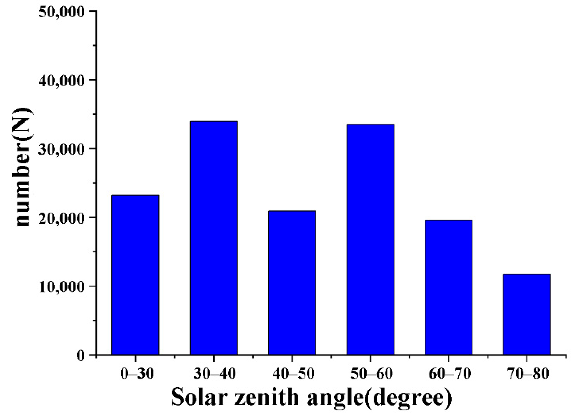
- After filtering the high-quality Rrs data, the Rayleigh-corrected radiance, SZA, observation zenith angle, and relative azimuth data with the same position in the 3-hour time window but large SZA (morning and evening hours) were used to match the noontime Rrs data. The size of the time window is the same as that proposed by the Marine Biological Processing Group for matching satellite and in situ data [29,30]. The distribution of the SZA in the final dataset is shown in Figure 2.
2.2.2. Building the HY-1C-COCTS Neural Network Atmospheric Correction Model
2.3. Statistical Parameters
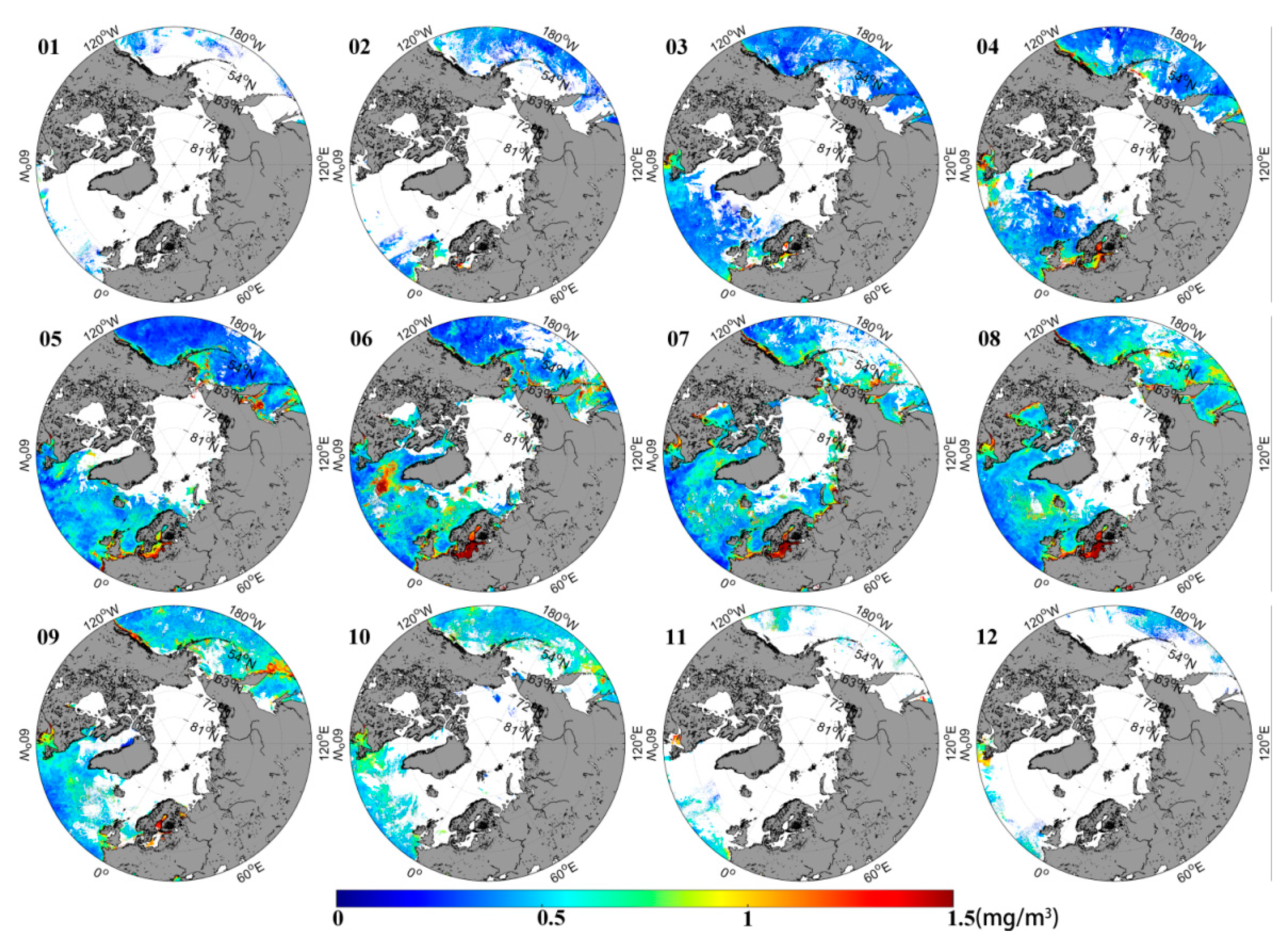
3. Results
3.1. Model Verification
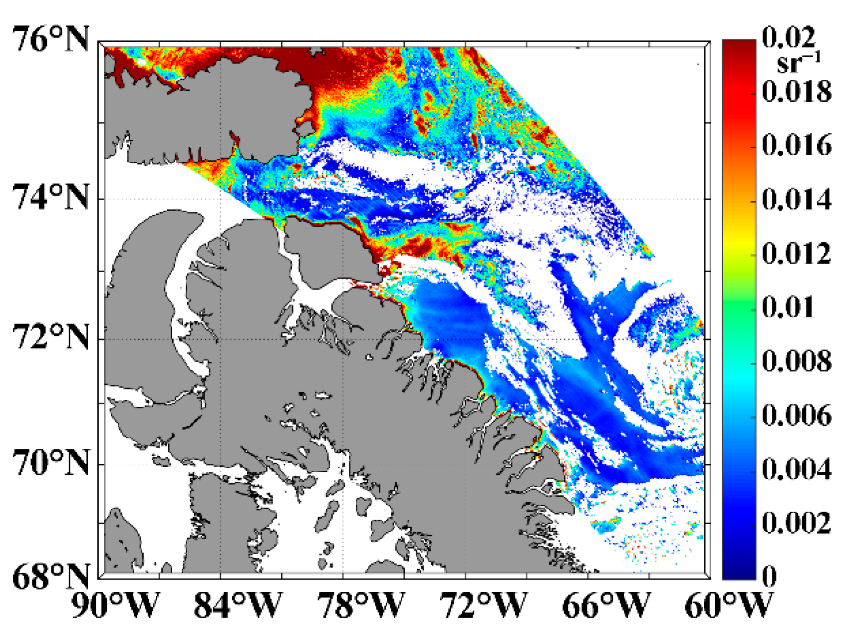
3.2. Cross Validation of Satellite Products
4. Discussion
5. Conclusions
Author Contributions
Funding
Data Availability Statement
Acknowledgments
Conflicts of Interest
References
- Liu, J.Q.; Zeng, T.; Liang, C.; Zou, Y.R.; Ye, X.M.; Ding, J.; Zou, B.; Shi, L.J.; Guo, M.H. Application of Ocean-1C Satellite in Natural Disaster Monitoring. Satell. Appl. 2020, 6, 26–34. [Google Scholar]
- Chen, S.; Du, K.; Lee, Z.; Liu, J.; Ma, C. Performance of COCTS in global ocean color remote sensing. IEEE Trans. Geosci. Remote Sens. 2020, 59, 1634–1644. [Google Scholar] [CrossRef]
- Lu, Y.C.; Liu, J.Q.; Ding, J.; Shi, J.; Chen, J.Y.; Y, X.M. Optical remote sensing identification of oil spill pollution type of the “Sangji” ship in the East China Sea. Chin. Sci. Bull. 2019, 64, 10. [Google Scholar]
- Shen, Y.F.; Liu, J.Q.; Ding, J.; Jiao, J.N.; Sun, S.J.; Lu, Y.C. Analysis of the oil spill recognition ability of Haiyang-1C star optical payload. Chin. J. Remote Sens. 2020, 24, 933–944. [Google Scholar]
- Li, H.; He, X.Q.; Bai, Y.; Shanmugam, P.; Huang, H. Atmospheric correction of geostationary satellite ocean color data under high solar zenith angles in open oceans. Remote Sens. Environ. 2020, 249, 112022. [Google Scholar] [CrossRef]
- He, X.Q.; Pan, D.L.; Bai, Y.; Mao, Z.; Wang, T.; Hao, Z. A Practical Method for On-Orbit Estimation of Polarization Response of Satellite Ocean Color Sensor. IEEE Trans. Geosci. Remote Sens. 2016, 54, 1967–1976. [Google Scholar] [CrossRef]
- Ruddick, K.G.; Ovidio, F.; Rijkeboer, M. Atmospheric correction of SeaWiFS imagery for turbid coastal and inland waters. Appl. Opt. 2000, 39, 897–912. [Google Scholar] [CrossRef] [Green Version]
- Wang, M.; Son, S.H.; Wei, S. Evaluation of MODIS-SWIR and NIR-SWIR atmospheric correction algorithms using SeaBASS data. Remote Sens. Environ. 2009, 113, 635–644. [Google Scholar] [CrossRef]
- Wang, M.; Wei, S. The NIR-SWIR combined atmospheric correction approach for MODIS ocean color data processing. Opt. Express 2007, 15, 15722–15733. [Google Scholar] [CrossRef] [Green Version]
- Li, H.; He, X.Q.; Shanmugam, P.; Bai, Y.; Wang, D.; Huang, H. Radiometric sensitivity and signal detectability of ocean color satellite sensor under high solar zenith angles. IEEE Trans. Geosci. Remote Sens. 2019, 57, 8492–8505. [Google Scholar] [CrossRef]
- Li, H.; He, X.Q.; Shanmugam, P.; Bai, Y.; Wang, D.; Huang, H. Semi-analytical algorithms of ocean color remote sensing under high solar zenith angles. Opt. Express 2019, 27, 800–817. [Google Scholar] [CrossRef] [PubMed]
- Meister, G.; Franz, B.A.; Kwiatkowska, E.J.; Mcclain, C.R. Corrections to the calibration of modis aqua ocean color bands derived from seawifs data. IEEE Trans. Geosci. Remote Sens. 2011, 50, 310–319. [Google Scholar] [CrossRef]
- Delgado, A.L.; Guinder, V.A.; Dogliotti, A.I.; Zapperi, G.; Pratolongo, P.D. Validation of modis-aqua bio-optical algorithms for phytoplankton absorption coefficient measurement in optically complex waters of EL RINCON(Argentina). Cont. Shelf Res. 2018, 173, 73–86. [Google Scholar] [CrossRef]
- Seegers, B.N.; Richard, P.S.; Blake, A.S.; Loftin, K.A.; Werdell, P.J. Performance metrics for the assessment of satellite data products: An ocean color case study. Opt. Express 2018, 26, 7404–7422. [Google Scholar] [CrossRef] [PubMed] [Green Version]
- Chen, J.; Cui, T.; Ishizaka, J.; Lin, C. A neural network model for remote sensing of diffuse attenuation coefficient in global oceanic and coastal waters: Exemplifying the applicability of the model to the coastal regions in Eastern China Seas. Remote Sens. Environ. 2014, 12, 22–25. [Google Scholar] [CrossRef]
- Marzano, F.S.; Iacobelli, M.; Orlandi, M.; Cimini, D. Coastal water remote sensing from sentinel-2 satellite data using physical, statistical, and neural network retrieval approach. IEEE Trans. Geosci. Remote Sens. 2020, 59, 915–928. [Google Scholar] [CrossRef]
- Fan, Y.; Li, W.; Gatebe, C.K.; Jamet, C.; Zibordi, G.; Schroeder, T. Atmospheric correction over coastal waters using multilayer neural networks. Remote Sens. Environ. 2017, 199, 218–240. [Google Scholar] [CrossRef]
- Fan, Y.; Chen, N.; Li, W.; Ahn, J.H.; Stamnes, K. Oc-smart: A machine learning based data analysis platform for satellite ocean color sensors. Remote Sens. Environ. 2020, 253, 112236. [Google Scholar] [CrossRef]
- Tian, X.J. Atmospheric correction of GOCI imaging neural network in turbid water bodies in the Bohai Sea. J. Hubei Univ. Nat. Sci. Ed. 2014, 36, 5. [Google Scholar]
- Shanmugam, P. CAAS: An atmospheric correction algorithm for the remote sensing of complex waters. Ann. Geophys. 2012, 30, 203–220. [Google Scholar] [CrossRef]
- Shen, J.P.; Wang, D.Y. Atmospheric correction of class II water bodies based on neural network. Geospat. Inf. 2019, 17, 5. [Google Scholar]
- Ling, S.; Jie, Z.; Sun, L. Atmospheric correction over case 2 waters using neutral network. J. Remote Sens. 2007, 11, 398–405. [Google Scholar]
- Chen, J.; He, X.Q.; Chen, B.; Pan, D.L. Deriving colored dissolved organic matter absorption coefficient from ocean color with a neural quasi-analytical algorithm. J. Geophys. Res. Ocean 2017, 10, 13–35. [Google Scholar] [CrossRef]
- Chen, J.; Quan, W.T.; Cui, T.W.; Song, Q.J.; Lin, C.S. Remote sensing of absorption and scattering coefficient using neural network model: Development, validation, and comparison. Remote Sens. Environ. 2014, 149, 213–226. [Google Scholar] [CrossRef]
- Chen, J.; Cui, T.W.; Joji, I.; Lin, C.S. A neural network model for remote sensing of diffuse attenuation coefficient in global oceanic waters. Remote Sens. Environ. 2014, 148, 168–177. [Google Scholar] [CrossRef]
- He, X.Q.; Stamnes, K.; Bai, Y.; Li, W.; Wang, D. Effects of earth curvature on atmospheric correction for ocean color remote sensing. Remote Sens. Environ. 2018, 209, 118–133. [Google Scholar] [CrossRef]
- He, X.Q.; Bai, Y.; Zhu, Q.; Gong, F. A vector radiative transfer model of coupled ocean–atmosphere system using matrix-operator method for rough sea-surface. J. Quant. Spectrosc. Radiat. Transf. 2010, 111, 1426–1448. [Google Scholar] [CrossRef]
- Gordon, H.R.; Wang, M. Retrieval of water-leaving radiance and aerosol optical thickness over the oceans with SeaWiFS: A preliminary algorithm. Appl. Opt. 1994, 33, 443–452. [Google Scholar] [CrossRef]
- Bailey, S.W.; Werdell, P.J. A multi-sensor approach for the on-orbit validation of ocean color satellite data products. Remote Sens. Environ. 2006, 102, 12–23. [Google Scholar] [CrossRef]
- Guanter, L.; Ruiz-Verdú, A.; Odermatt, D.; Giardino, C.; Simis, S.; Estellés, V.; Heege, T.; Domínguez-Gómez, J.A.; Moreno, J. Atmospheric correction of ENVISAT/MERIS data over inland waters: Validation for european lakes. Remote Sens. Environ. 2010, 114, 467–480. [Google Scholar] [CrossRef] [Green Version]
- Gross, L.; Thiria, S.; Frouin, R. Applying artificial neural network methodology to ocean color remote sensing. Ecol. Model. 1999, 120, 237–246. [Google Scholar] [CrossRef]
- Chen, S.; Hu, C.; Barnes, B.B.; Xie, Y.; Lin, G.; Qiu, Z. Improving ocean color data coverage through machine learning. Remote Sens. Environ. 2019, 222, 286–302. [Google Scholar] [CrossRef]
- O’Reilly, J.E.; Maritorena, S.; Siegel, D.A.; O’Brien, M.C.; Toole, D.; Mitchell, B.G.; Culver, M. Ocean color chlorophyll a algorithms for SeaWiFS, OC2, and OC4: Version 4. SeaWiFS Postlaunch Calibration Valid. Anal. 2000, 3, 9–23. [Google Scholar]


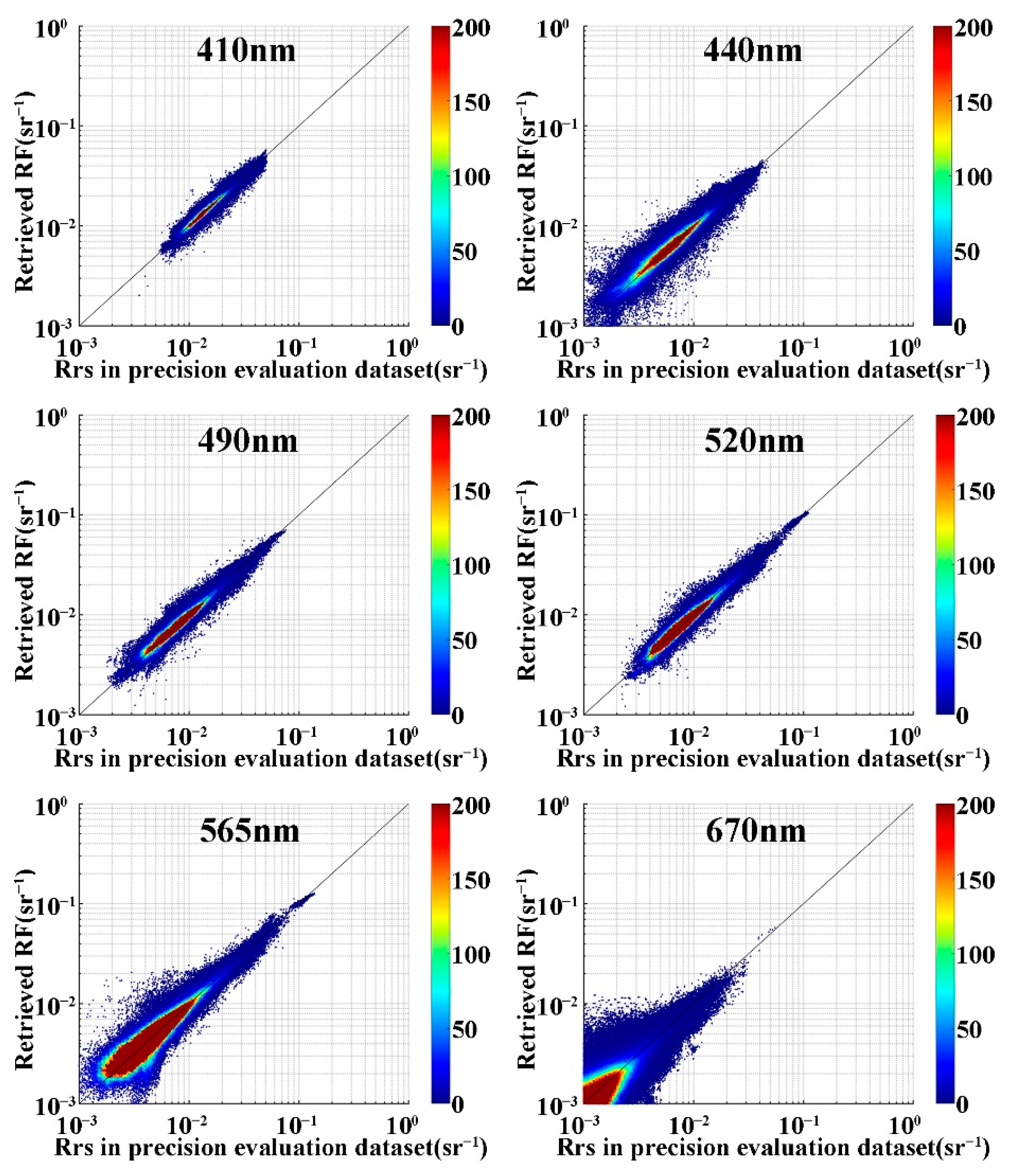
| Band | RMSD (sr−1) | APD (%) | RPD (%) |
|---|---|---|---|
| 412 nm | 0.00075 | 0.45% | 3.37% |
| 443 nm | 0.00079 | 1.15% | 7.05% |
| 490 nm | 0.00069 | 0.22% | 5.10% |
| 520 nm | 0.00070 | 0.14% | 5.29% |
| 565 nm | 0.00080 | −0.37% | 10.06% |
| 670 nm | 0.00071 | 26.12% | 48.68% |
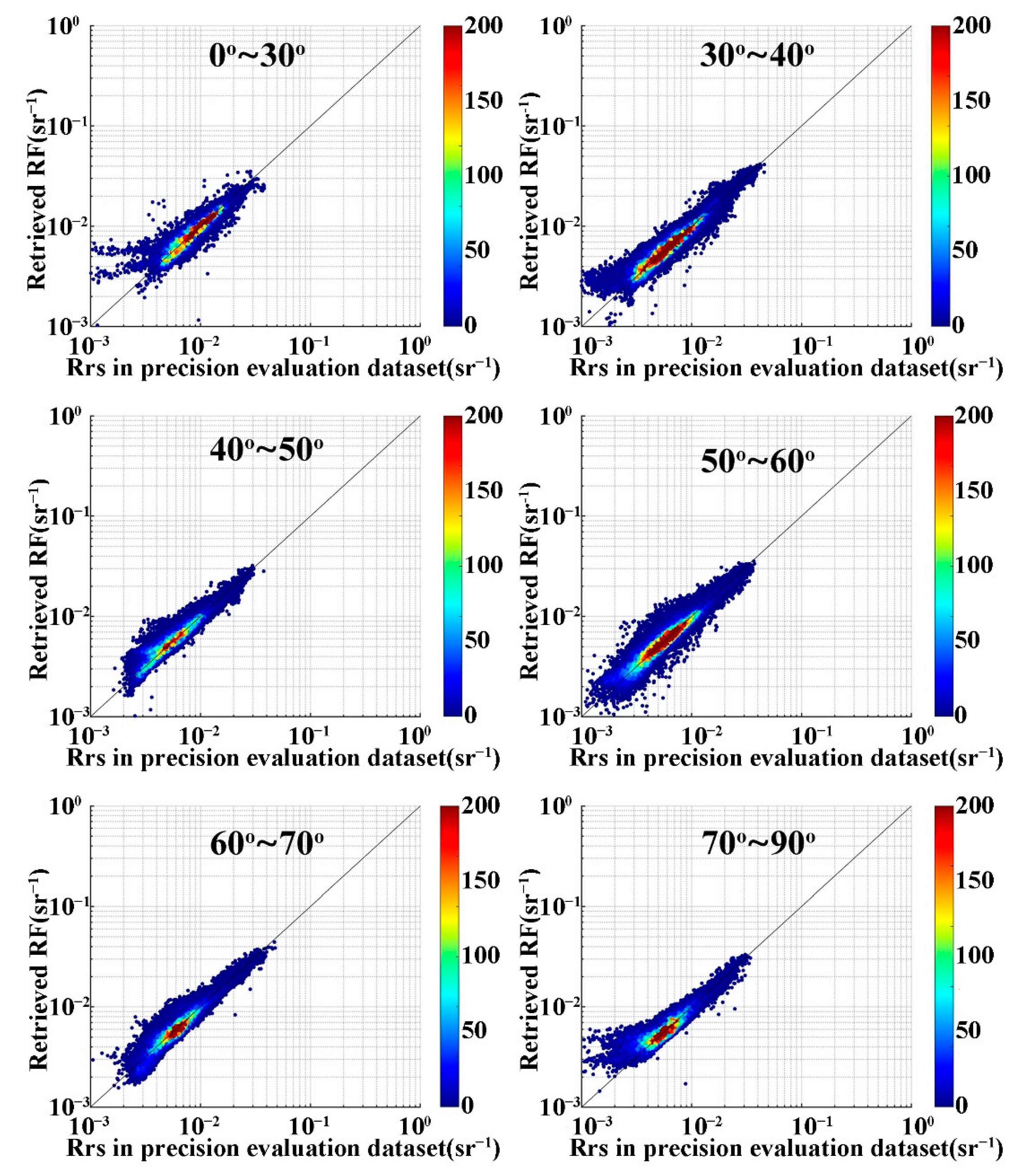
| SZA | RMSD (sr−1) | APD (%) | RPD (%) |
|---|---|---|---|
| 0~30° | 0.00078 | 0.89% | 5.95% |
| 30~40° | 0.00073 | 0.70% | 6.80% |
| 40~50° | 0.00077 | 2.56% | 8.57% |
| 50~60° | 0.00091 | 1.44% | 8.85% |
| 60~70° | 0.00060 | 0.26% | 3.83% |
| 70~90° | 0.00028 | 0.44% | 1.07% |
Publisher’s Note: MDPI stays neutral with regard to jurisdictional claims in published maps and institutional affiliations. |
© 2022 by the authors. Licensee MDPI, Basel, Switzerland. This article is an open access article distributed under the terms and conditions of the Creative Commons Attribution (CC BY) license (https://creativecommons.org/licenses/by/4.0/).
Share and Cite
Li, H.; He, X.; Ding, J.; Bai, Y.; Wang, D.; Gong, F.; Li, T. The Inversion of HY-1C-COCTS Ocean Color Remote Sensing Products from High-Latitude Seas. Remote Sens. 2022, 14, 5722. https://doi.org/10.3390/rs14225722
Li H, He X, Ding J, Bai Y, Wang D, Gong F, Li T. The Inversion of HY-1C-COCTS Ocean Color Remote Sensing Products from High-Latitude Seas. Remote Sensing. 2022; 14(22):5722. https://doi.org/10.3390/rs14225722
Chicago/Turabian StyleLi, Hao, Xianqiang He, Jing Ding, Yan Bai, Difeng Wang, Fang Gong, and Teng Li. 2022. "The Inversion of HY-1C-COCTS Ocean Color Remote Sensing Products from High-Latitude Seas" Remote Sensing 14, no. 22: 5722. https://doi.org/10.3390/rs14225722