Article

Anomalous Zenith Total Delays for an Insular Tropical Location: The Tahiti Island Case

1
College of Geodesy and Geomatics, Shandong University of Science and Technology, Qingdao 266590, China
2
Department of Space, Earth and Environment, Chalmers University of Technology, Onsala Space Observatory, SE-439 92 Onsala, Sweden
3
Harbin Institute of Technology, Shenzhen 518055, China
4
Geodesy Observatory of Tahiti, University of French Polynesia, 98702 Faa’a, French Polynesia
*
Author to whom correspondence should be addressed.
Remote Sens. 2022, 14(22), 5723; https://doi.org/10.3390/rs14225723
Submission received: 19 October 2022 / Revised: 9 November 2022 / Accepted: 10 November 2022 / Published: 12 November 2022
(This article belongs to the Special Issue Precision Orbit Determination of Satellites)

Abstract

:
The weighted mean temperature of the troposphere, Tm, is a key parameter in GNSS meteorology. It can be routinely derived based on meteorological data from radiosonde (RS) or numerical weather models. Alternatively, it can be also derived through a least-squares model of the ratio between the precipitable water vapor from RS data and the zenith wet delay estimates from GNSS measurement in the precise point positioning mode. In this last case, we found anomalous Tm values for the remote sub-tropical humid location of the Tahiti Island in the South Pacific Ocean and traced these anomalous values to anomalous zenith total delays (ZTD) that seem to have an accuracy poorer by one order of magnitude than the claimed accuracy of ZTD delays from worldwide databases. The possible causes of these discrepancies are discussed.

1. Introduction

The atmospheric water vapor plays a central role in all meteorology/climate processes, and at all temporal and spatial scales: micrometeorology, evapotranspiration, clouds, precipitations, and energy balance [1]. In addition, water vapor accounts for around three quarters of the greenhouse warming on Earth, and is therefore one of the main drivers of climate variability [2]. Precipitable water vapor (PWV/PW), the core quantity to model the water vapor contents of the troposphere, is defined as the equivalent amount of water that could be produced if all the water vapor in an atmospheric column rained down instantly [3].
Several techniques are commonly used to model the spatial and temporal variations of PW. These include radiosonde balloons (RS), water vapor radiometers, and sun photometers, but their low spatial and temporal resolution, and sometimes poor quality and high cost limit their use [4,5,6,7]. To overcome these drawbacks, the ground-based Global Positioning System (GPS) receivers, and now GLONASS, BDS, and Galileo (collectively known as Global Navigation Satellite Systems (GNSS)) have been extensively used since the early 1990s for the determination of PW with all-weather capability, high temporal sampling frequency (down to a few minutes), and widely different line-of-sight receiver-satellite geometries (from the near-horizon to zenith direction) [8]. Widely used techniques include relative positioning and precise point positioning (PPP). Compared to relative positioning, PPP is favored in GNSS meteorology because it uses a stand-alone receiver to obtain absolute atmospheric parameters [9]. The GNSS receivers are also relativity cheap, with the average cost of a GNSS receiver being roughly equivalent to 25 radiosonde balloon launches [10].
An extra atmospheric delay in the GNSS receiver-satellites radio-links is caused, at around a 10–20% level, by the wet refractivity variations in the troposphere, with the bending of the ray as a second order effect [11,12]. The wet refractivity is highly variable, both horizontally and vertically. The total propagation delay, remapped along the vertical direction, is named zenith total delays (ZTD). It can be split as the sum of a zenith hydrostatic (also improperly called “dry”) delay (ZHD) and a zenith wet (non-hydrostatic) delay (ZWD) [13]. The ZHD can be determined with a good accuracy by empirical models such as the Hopfield model [14], the Saastamoinen model [15], or the Black model [16]; all of them are constrained by surface meteorological measurements (temperature and pressure). Therefore, the ZWD can be defined by the relation ZWD = ZTD-ZHD, if we assume no other factors other than water vapor are involved. The PW itself can be derived from the ZWD by using a multiplicative conversion factor, a function of the so-called weighted mean temperature Tm [17,18]. Usually, values of Tm are derived by analyzing long time series of RS profile observations, but they can also be computed by ray tracing/vertical integration with respect to gridded numerical weather models (NWM) [19,20]. In 1992, Bevis et al. demonstrated that there is a linear relation between Tm and Ts (Tm = a + b·Ts), with Tm < Ts. The surface temperature, Ts, can be easily obtained from GNSS collocated weather stations or nearby weather stations (for example, [21] for Europe, [22] for India, [23] for Turkey, and [24] for Tahiti). To improve the reliability of GNSS PWV, Huang et al. (2022) adopted three enhanced vertical correction models for temperature, pressure, and PWV, and developed four accurate Tm models suitable for four regions of China [25]. Ross and Rosenfeld (1997) noted that the coefficients of the linear relationship between Tm and Ts change as a function of locations and seasons [26]. In other words, PW estimates from GNSS data need three input values: ZTD, ZHD, and Tm, and a site-dependent tailored fit [27,28].
This study was prompted by the conclusions of a previous paper [24] about the determination of PW estimates in Tahiti from GPS data only, with stand-alone receivers used in the PPP mode. The linear fits TmTs pointed, in this tropical context, to overlarge values of Tm, sometimes larger than the surface temperature Ts. From its own definition (see Equation (14)), Tm should be lower than the maximum temperature in the troposphere, normally found at ground level (a small inversion layer due to the trade winds present in Tahiti but does not change this behavior). The determination of the linear fit was also complicated by the fact that the range of surface temperature in Tahiti is also quite limited, around 10 K, thanks to the South Pacific Ocean acting as a heat buffer. This problem is already apparent in the seminal paper of Bevis et al. (1992) [29], where the scatter around the linear relationship TmTs becomes larger and larger with increasing values of Tm and Ts. In this previous paper, two possible conclusions were made: (1) the underlying physics of the TmTs linear relationship break for some reasons for large atmospheric humidity contents, and/or (2) some systematic errors are present in the GNSS data processing software or in the determination of Ts. The purpose of this follow-on paper is to investigate these two points by examining all the links of the computation chain leading to the mean temperature estimate. Our breadcrumb trail will be the comparison between the TmTs relationship determined from in situ RS/meteorological data and the TmTs relationship determined from GNSS data.
The paper is organized as follows: Section 2 recalls the underlying physics of the derivation of ZTD, ZHD, ZWD, Tm and PW; Section 3 introduces the datasets; Section 4 analyses the results, including comparisons between our results and the references; Section 5 gives the discussion about the anomalous ZTD results; and Section 6 draws the conclusions.

2. Methodology

The total tropospheric delay along the zenith direction can be determined as the integration along the vertical of the atmospheric total refractivity N as:
Z T D = 10 6   N   d z ,
where z is the geometrical height of the observation site above the mean sea level. N and its subparts Nd (hydrostatic) and Nw (wet) can be written as:
N = k 1 ( P d T ) Z d 1 + k 2 ( P v T ) Z v 1 + k 3 ( P v T 2 ) Z v 1 = N d + N w ,
N d = k 1 ( P T ) Z d 1 ,
N w = [ k 2 ( P v T ) + k 3 ( P v T 2 ) ] Z v 1 ,
where T is the temperature in Kelvin, Pd is the dry air pressure in mbar, Pv the water vapor pressure in mbar [30], and P = Pd + Pv. Z d 1 and Z v 1 are the inverse compressibility factors for dry air and water vapor, respectively [31]. Nd is the refractivity of dry air and Nw is the refractivity of water vapor. k1, k2 and k3 are refractivity constants, k 2 = k2k1·(Mw/Md) = 22.1 (K/hPa), Mw = 18.0152 (kg/kmol) is the molar weight of wet air, and Md = 28.9644 (kg/kmol) is the molar weight of dry air [19].
As ZTD is, by its own definition, equal to the sum of ZHD and ZWD [29], then:
Z H D = 10 6 N d   d z = 10 6 k 1 ( P T ) Z d 1   d z ,
and
Z W D = 10 6 N w   d z = 10 6 k 2 ( P v T ) Z v 1   d z + 10 6 k 3 ( P v T 2 ) Z v 1   d z ,
From an observational point of view, Pv is measured as
P v = R H · e s / 100 ,
where RH is the sensor relative humidity, and es is the saturation water vapor pressure that depends on the surface temperature Ts [32,33], that can be calculated by
e s = 6.11 × 10 7.5 × T s 237.3 + T s .
The ZHD must always be calculated from empirical models as the signature of the water vapor in the ZTD cannot be distinguished, from a practical point of view, from the signature in the hydrostatic delay (ZHD) [34]. The Saastamoinen model is the most common model, with an accuracy that is claimed to be at the millimeter-level [15]:
Z H D = 2.2779   P s / f ( λ ,   H ) ,
The model of [17] has the same form as the Saastamoinen model, but with a slightly different constant:
Z H D = 2.2768   P s / f ( λ ,   H ) ,
where, for both, f(λ,H) = 1 – 0.00266·cos(2λ) – 0.00028·H, H(km) is the geometrical height of the receiver above the ellipsoid, λ(rad) is the station latitude, and Ps is the surface pressure in hPa.
As already stated, ZWD is defined as the Equation (11):
Z W D = Z T D Z H D ,
with ZWD converted into PW by [19]:
P W = Π · Z W D ,
and with the ratio Π defined as [35]:
Π = 10 6 / ( ρ · R v ( k 3 T m + k 2 ) ) ,
where ρ = 1000 (kg/m3) is the density of liquid water (kg/m3), and Rv = 461.495 (J/kg·K) is the specific water vapor constant. Tm, the vertically weighted mean temperature of the atmosphere with respect to its water vapor contents, is defined as [17]:
T m = ( P v / T ) d z / ( P v / T 2 ) d z ,
As it is clear from Equation (14), time series of Tm for a particular site can be derived from the knowledge of the vertical values of T and Pv from RS profiles or numerical weather models [20]. It is also clear from Equation (14) that Tm is the mean temperature defined with the water vapor pressure Pv as weight. It should be also emphasized that this definition ignores any orographic effect, with the exception of the initial altitude of the vertical profiles.
RS profiles and gridded weather models also allow a direct computation of PW as:
P W = 1 ρ   ρ w d z ,
ρ w = P v / ( R v · T ) ,
where ρw is the density of water vapor.

3. Datasets

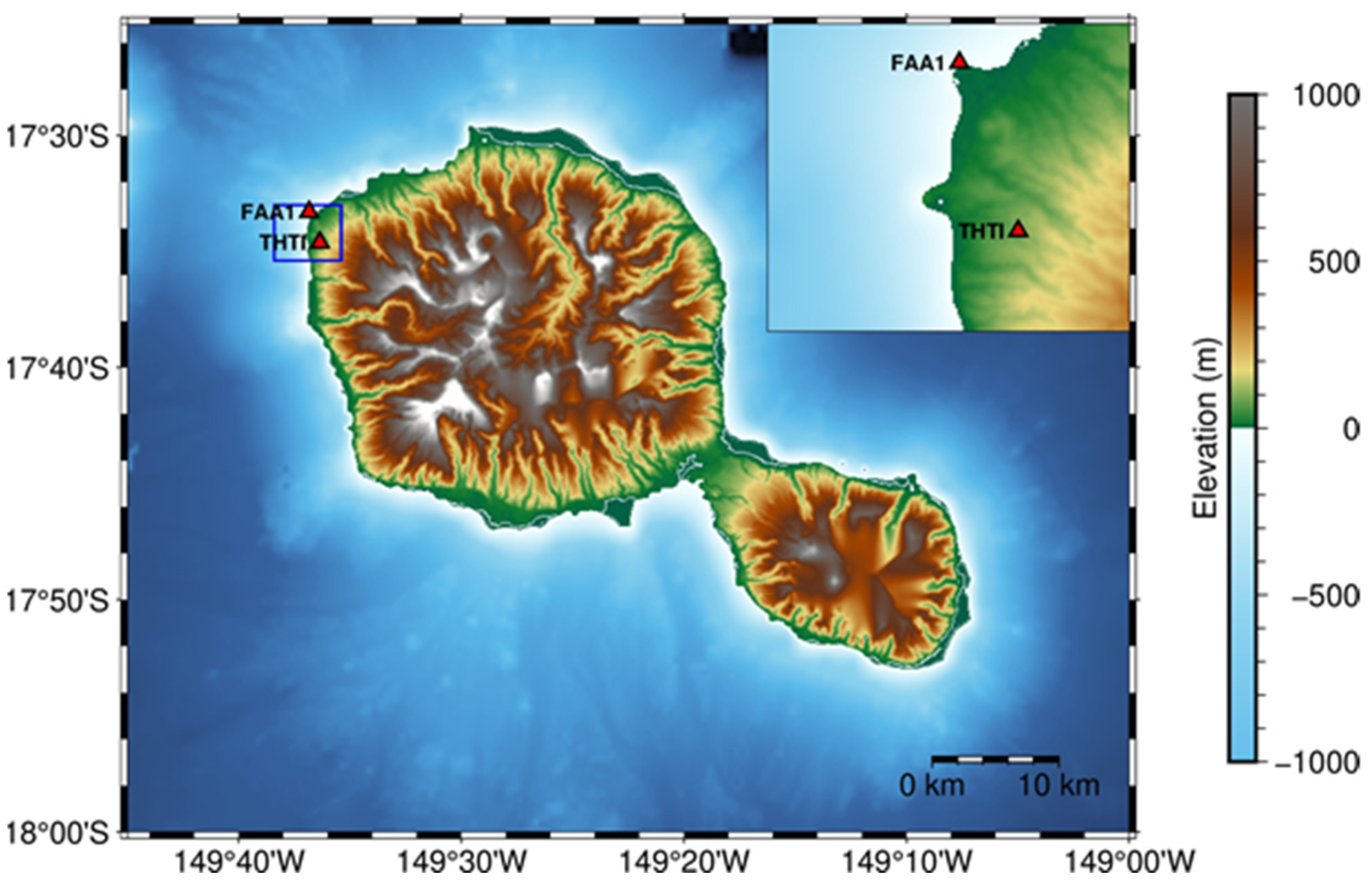
Two International GNSS Service (IGS) stations are operating on the South Pacific Ocean Island of Tahiti: FAA1 is located at almost sea level on the premises of the Tahiti international airport; THTI is located inland at a horizontal distance of 2.56 km and with an altitude difference of 86.14 m with respect to FAA1. Although they are close (Figure 1), their surroundings are quite different. FAA1, managed by Météo-France, is located at near sea-level, under the premises of the international airport, on a very large area that was flattened to host the airstrip. THTI is located on the main campus of the University of French Polynesia, a little bit more inland, on a ridge crest with a slope of about 8%, at a distance from the sea of about 1.5 km. They belong to two distinct valleys, each one with its own micro-climate [10,36].
A precise analysis of the differences between their ZTD time series showed that the difference in insulation (and so evapotranspiration), and not the altitude difference, is the leading actor in these differences. For this study, we processed GNSS data for the whole year of 2017 on a daily basis, and obtained one-year ZTD results using the Bernese Software Version 5.2 in the static post-processing PPP mode [37,38]. To validate the accuracy of our ZTD estimates, we compared our estimates with the Center for Determination in Europe (CODE) tropospheric products and the IGS final tropospheric products. Their ZTD products, with a claimed accuracy of 4 mm, are presented in the literature [39,40] as highly reliable products. Details of these data processing strategies are described in Table 1.
The Integrated Global Radiosonde Archive (IGRA) is maintained by the National Oceanic and Atmospheric Administration (NOAA) and consists of radiosonde observations over 2700 globally distributed stations since 1905 [42]. A IGRA radio sounding balloon station is collocated with the FAA1 GNSS receiver at a few meters distance. The RS balloons are launched twice a day at 00:00 and 12:00 UTC and provide approximately vertical profiles (depending on the wind) of the atmospheric key variables including pressure, temperature, relative humidity, wind speed and direction, dew point temperature, and elapsed time since launch, until the balloon blows up under overpressure of its envelope at around 30 km [43].
The meteorological parameters from the site-wise VMF1 files (using the 40 years reanalysis (ERA-40) NWM data of the ECMWF, https://vmf.geo.tuwien.ac.at/, accessed on 9 November 2022) were also used in this study. The values are interpolated from a 2.0° × 2.5° grid, with a six-hour temporal resolution, and include the so-called hydrostatic/wet “a” coefficient of the VMF1 mapping function continuous fraction, the hydrostatic/wet zenith delays, an estimation of the atmosphere mean temperature above the site, the pressure, temperature and water vapor pressure at the site, and the orthometric altitude of the station (geoid model EGM96) [39]. Here, all site-wise products are generated based on the coordinates and altitude of IGS stations [44].
In addition, to compute tropospheric delays, we converted the geopotential heights recorded on RS data to orthometric heights [45]. The 1976 US Standard atmosphere [46] at waterless high altitudes was used to complement the RS troposphere delay models. This standard atmosphere model, up to 100 km altitude, assumes that air is a clean, dry (no water vapor present) gas, obeying the perfect gas law and the hydrostatic equation. It is roughly representative of year-round, mid-latitude conditions [47].

4. Results

In this section, to analyze and discuss our results calculated by using the above methodology and datasets, we make some comparisons between our results and the references that will be provided, including our ZTD estimates versus CODE and IGS products in Section 4.1, surface temperature from ground station versus that from site-wise VMF1 files in Section 4.2, weighted mean temperature estimated from RS measurements versus that from site-wise VMF1 files in Section 4.3, ZWD results estimated from RS measurements versus that from site-wise VMF1 files in Section 4.4, ZHD estimates based on the original Saastamoinen model versus that based on Davis’ adapted Saastamoinen model in Section 4.5, and Section 4.6 includes ZHD estimates based on Davis’ adapted Saastamoinen model versus that calculated by using RS data and standard atmosphere, and GPS ZTD estimates versus ZTD derived from RS data and standard atmosphere. The detailed comparisons are presented in the following.

4.1. Comparisons of Our ZTD Estimates with CODE and IGS ZTD Estimates

To validate the effectiveness of our data processing strategies and the accuracy of our ZTD estimates, we compare, in this subsection, our ZTD to CODE/IGS ZTD products. The different settings between our processing and CODE/IGS products are summarized in Table 1. Our processing and the IGS final ZTD products both use the so-called PPP post-processing mode [48,49]. IGS lists four PPP providers at the time of the writing of these lines (https://igs.org/products-access/#gps-orbits-clocks, accessed on 9 November 2022). Our Bernese 5.2 software uses the PPP-CODE final product (https://www.aiub.unibe.ch/research/code___analysis_center/, accessed on 9 November 2022) and the IGS data analysis centers use the PPP-IGS final product [50]. Details about what are exactly the differences in processing strategies between the currently available PPP products are arcane. We refer to [48,51,52] for recent assessments of the PPP models for several constellations. All these PPP products claim a few centimeter-level accuracy on the GPS satellite orbits. CODE ZTD products use the relative positioning approach [39].
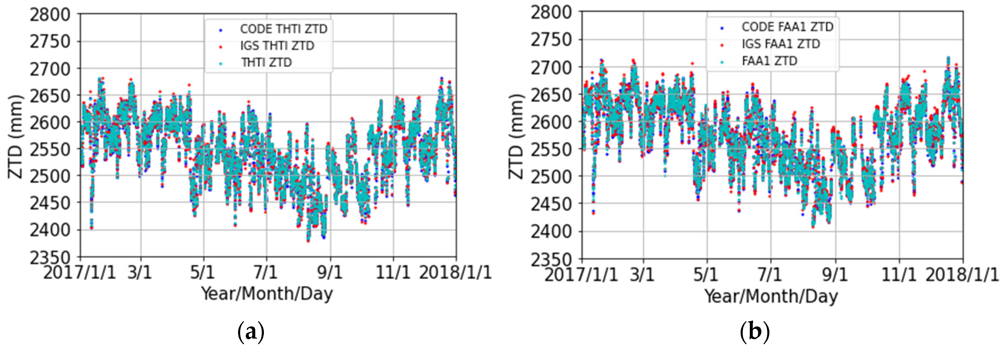
From a practical point of view, our ZTD estimates are very close to the CODE/IGS final ZTD products (Figure 2a,b and Table 2), with a mean bias at the mm level over one year, probably caused by some different settings between our GPS data processing and the CODE/IGS final products (Figure 2c,d): PPP/relative positioning models, mapping functions, a priori ZTD models, cut-off angles, and oceanic/Earth tides models (see Table 1). Such a small bias does not validate our processing versus CODE/IGS products. It just indicates that if systematic effects are present, they are present in both these computations, possibly disappearing in the ZTD differences.
According to Table 2, RMS values for the FAA1 site are larger than that for the THTI site, by around 3 mm. This difference is mainly driven by insolation differences, and the differences in altitude and the wind are secondary factors, as presented by Zhang et al. (2019) [10].

4.2. Comparison of the Surface Temperature from the FAA1 Ground Weather Station and the Site-Wise VMF1 Files

To assess from a metrological point of view, the linear relationship between the mean temperature, Tm, and surface temperature, Ts, we need to examine the accuracy of 
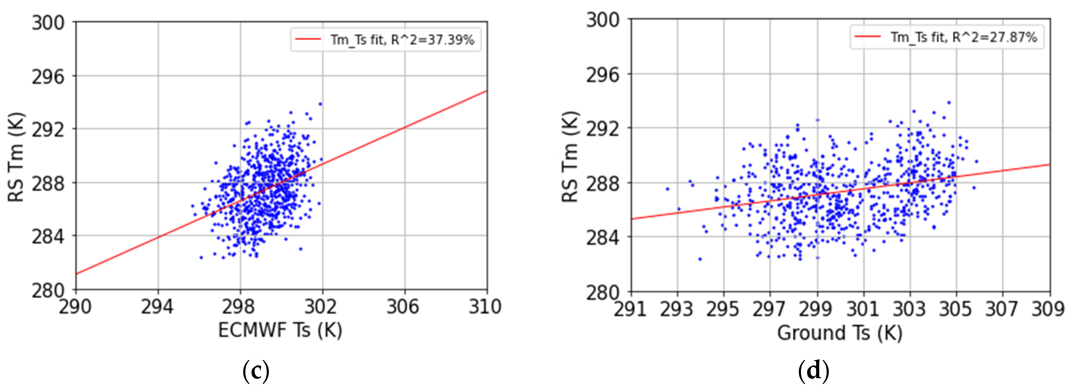
Ts values. For this purpose, we compared the surface temperature records (T1) from the FAA1 ground weather station with the time series of the surface temperature (T2) from the site-wise VMF1 files (Figure 3a). The histogram of the temperature differences between T1 and T2 is shown in Figure 3b. From time series of T2, we find that surface temperature over Tahiti is relatively stable with variations less than 8 K through one year, reaching the lowest values in August. T1 generally follows the trend of T2 but exhibits larger noises. According to Figure 3b, the noises of T1 roughly obey a Gaussian distribution with a small bias. A statistical summary provided in Table 3 shows that these two temperature records are coherent with a bias of 1 K and an RMS of 2 K. We should emphasize that ground temperatures are influenced by micro-scale variations, both in time and space, of turbulence and insolation at the air-soil interface, so the concept of “surface temperature” is a blurry one. These micro-scale variations are certainly the main contributor to the RMS value of 2 K.

4.3. Comparison of Tm Estimates from RS Measurements and Site-Wise VMF1 Files

In this section we derive mean temperature, Tm, estimates built only from the RS balloon measurements (noted RS − Tm) made at the FAA1 weather station in 2017. We calculated the Tm estimates by directly considering its definition (Equation (14)), with the flight of the balloon assumed to be vertical up to its maximum altitude. Its lateral drift can reach up to 20 to 50 km, depending on the direction and intensity of the wind [24].
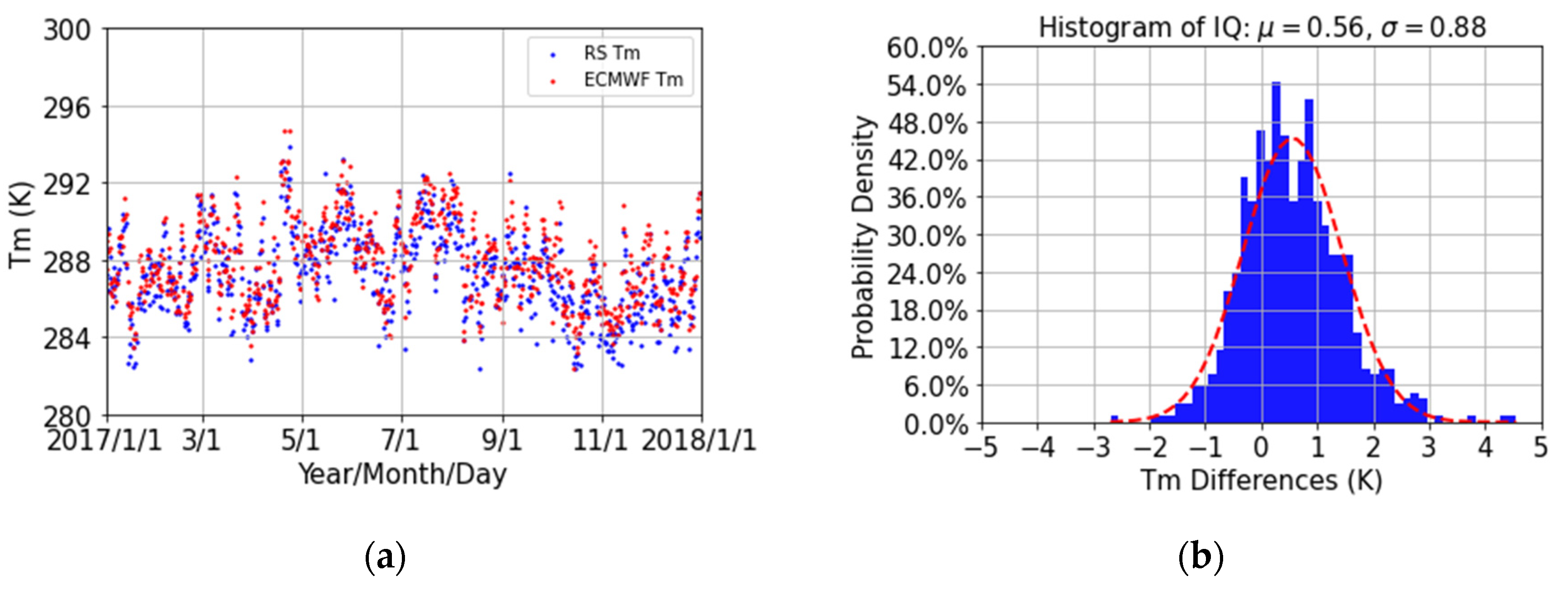
We compared our RS − Tm estimates with the Tm estimates from the site-wise VMF1/ECMWF files, that considers an atmospheric column up to 47 km [39]. Time series, histogram of their differences, and a statistical summary are given in Figure 4a,b and Table 4, respectively. According to Figure 4a, RS − Tm values are consistent with the VMF1 ones, displaying a periodical pattern with peak-to-peak values of around 8 K. From Table 4, the bias and RMS values of the differences between RS − Tm and Tm from VMF1/ECMWF are 0.56 K and 1.05 K, respectively.
We can now try to check a possible linear relationship noted TmTs, based on the FAA1 surface temperature estimates, Ts, from the site-wise VMF1/ECMWF files (Figure 4c) or the FAA1 ground weather station (Figure 4d) and our weighted mean temperature, Tm, from RS measurements. In Figure 4c, the linear relationship between Tm and Ts is shown based on 724 RS profiles as Tm = 0.69 × Ts + 81.99, with R2 = 37.39% and an error bar of 6.01 K. In Figure 4d, the linear relationship between Tm and Ts is shown based on 724 RS profiles as Tm = 0.22 × Ts + 220.56, with R2 = 27.879% and an error bar of 6.22 K. Clearly, these fits are not good. We think that the main culprit is the small range of surface temperature, Ts, (10 K) in Tahiti over the year [24] that impairs a reliable estimation of the fit line, probably linked with instrumental difficulties for the balloon humidity sensor to measure accurately the high levels of water vapor present in the tropical location of Tahiti (Equation (7), see [53]).

4.4. Comparison of the ZWD Estimates from RS Data with the ZWD Estimates from VMF1/ECMWF Files

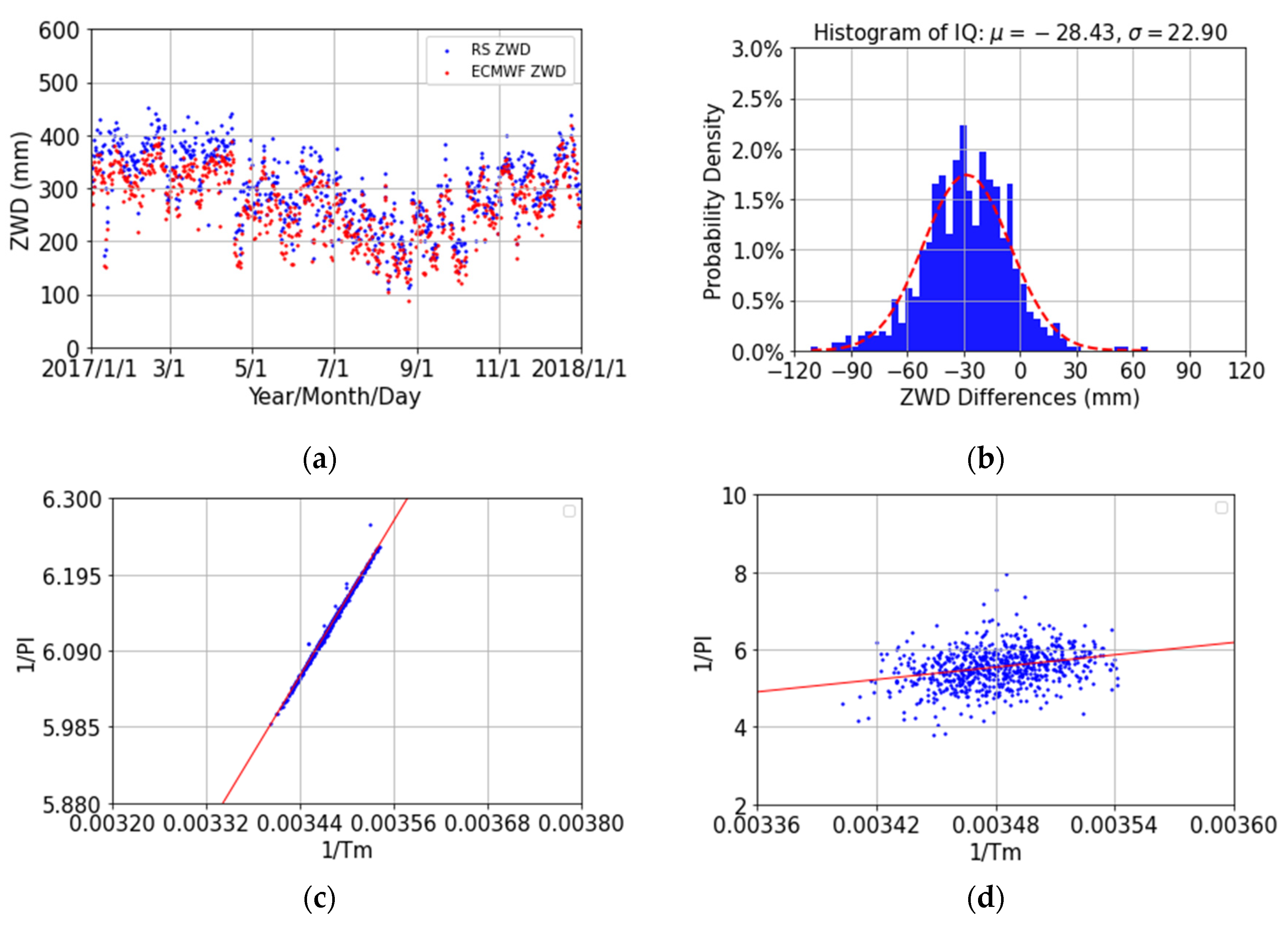
The next step is to compare our ZWD estimates from RS data (RS-ZWD) with ZWD estimates from VMF1/ECMWF records (VMF1/ECMWF-ZWD) for the FAA1 site. Our RS-ZWD estimates at the FAA1 station were calculated by using Equation (6). In our case, we did not consider the extension of the atmospheric column by the standard atmosphere, as it is void by construction of any water vapor. In Figure 5a, the consistency between the RS-ZWD and the VMF1/ECMWF-ZWD is also not very good, with an obvious bias of 28.43 mm (Table 5). In addition, the RMS between our RS-ZWD and VMF1/ECMWF-ZWD is also very large at about 34.57 mm (Table 5). Indicated by [39,54], the ZWD differences between ZWD estimates obtained from the VMF1/ECMWF files and ZWD derived by GPS data processing are very large in terms of bias and STD up to a 2-cm level for the Kokee Park station (Kaua’i Island, Hawaii), with a climatic environment close to the one found in Tahiti.
We conclude that for the FAA1 station (and Kokee Park station), with a very high humidity, the large biases of Table 5 are mainly the result of a mismodeling of the wet contents of the atmosphere from the underlying numerical weather models, probably due to micro-local effects, as the resolution of the site-wise VMF1/ECMWF files (more than 200 km) is much larger than the dimensions of the Tahiti Island (30 km in diameter) or Kaua’i Island (35 km in diameter).
We then tested if the computation of the Π factor through Equation (13) is valid. For this purpose, we plotted, for the FAA1 station, the relation between 1/Π and 1/Tm that should be linear according to this equation. Based on Equation (12), the 1/Π factor can be estimated using a ZWD estimate divided by the corresponding PW estimate. This is indeed the case with a very high accuracy with RS – ZWD and RS – PW calculated through Equation (15) (Figure 5c, with 1/Π noted 1/Π1). The linear relationship between 1/Π1 and 1/Tm (Tm values are also from the RS measurements) is shown based on 724 RS profiles as 1/Π1 = 1779.61 × 1/Tm − 0.07, with R2 = 99.78% and an error bar of 0.01 K. Besides, we estimated 1/Π using GPS (VMF1/ECMWF)-ZWD divided by RS – PW (Figure 5d, with 1/Π noted 1/Π2). We have 1/Π2 = 5322.56 × 1/Tm − 12.98, with R2 = 28.38% and an error bar of 1.41 K.
The conclusion is straightforward; the underlying physics for the TmTs relationship is confirmed, even for the high levels of humidity found in Tahiti. We have to look at other possible causes for the violation of Tm < Ts.

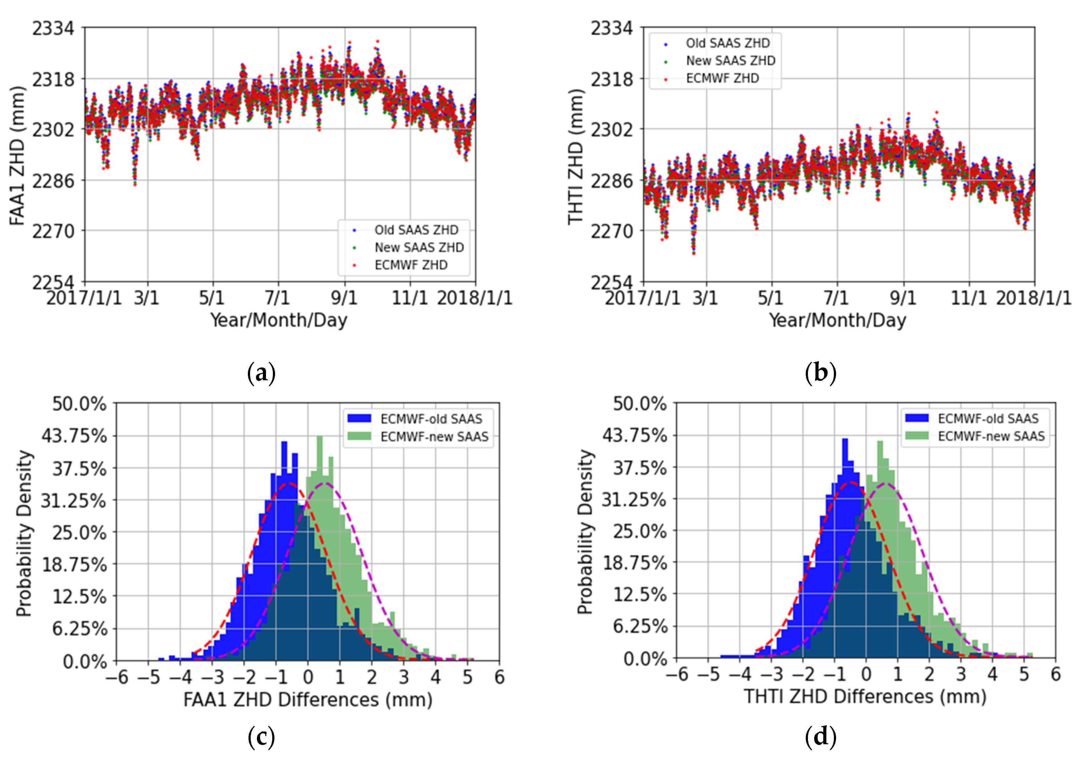
4.5. Comparison of ZHD Estimates Based on the Saastamoinen Model with ZHD Estimates Based on Davis’ Adapted Saastamoinen Model

The two most used empirical models, with an accuracy that is claimed to be at the mm-level for the determination of ZHD estimates, the Saastamoinen model (1972, Equation (9), noted here old-SAAS) and the Davis-Saastamoinen model, as modified by Davis et al. (1985, Equation (10), noted here new-SAAS), are analyzed in this section.
We used the VMF1/ECMWF pressure time-series for the FAA1 (Figure 6a,c) and THTI (Figure 6b,d) IGS stations, that are separated by a 2.56 km horizontal distance and an altitude difference of 86.14 m [10], to calculate ZHD estimates with respect to the two kinds of Saastamoinen models. A statistical summary is given in Table 6. For both stations, the ZHD estimates from the two kinds of Saastamoinen models are consistent with the ZHD VMF1/ECMWF estimates at the mm level.
Zhang et al. (2016) [55] increased the numerator value in Equation (10) from 2.26768 to 2.2794 and claimed a global ZHD accuracy of less than 1 mm for this modified formula. This is certainly not true for our case, as this model is leading to a larger bias because of the large value in the numerator with respect to the Saastamoinen original and modified formulas.

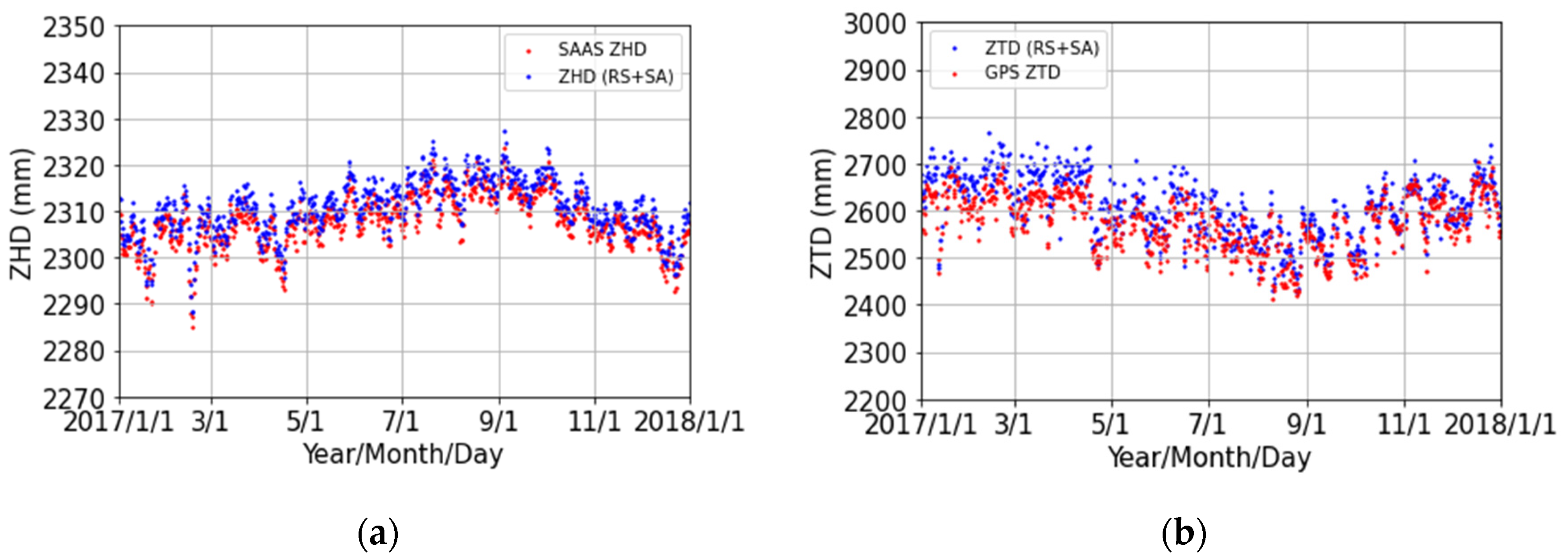
4.6. Comparison of GPS ZTD Estimates with ZTD Estimates from RS Data and a Standard Atmosphere

In this section, based on Equation (5), we first calculate the ZHD estimates by using RS data from the surface of the Earth up to a balloon altitude of 30 km, and then we complement this value up to a 100 km altitude by using the vertical profiles from the U.S. Standard Atmosphere (SA) 1976 model [46].
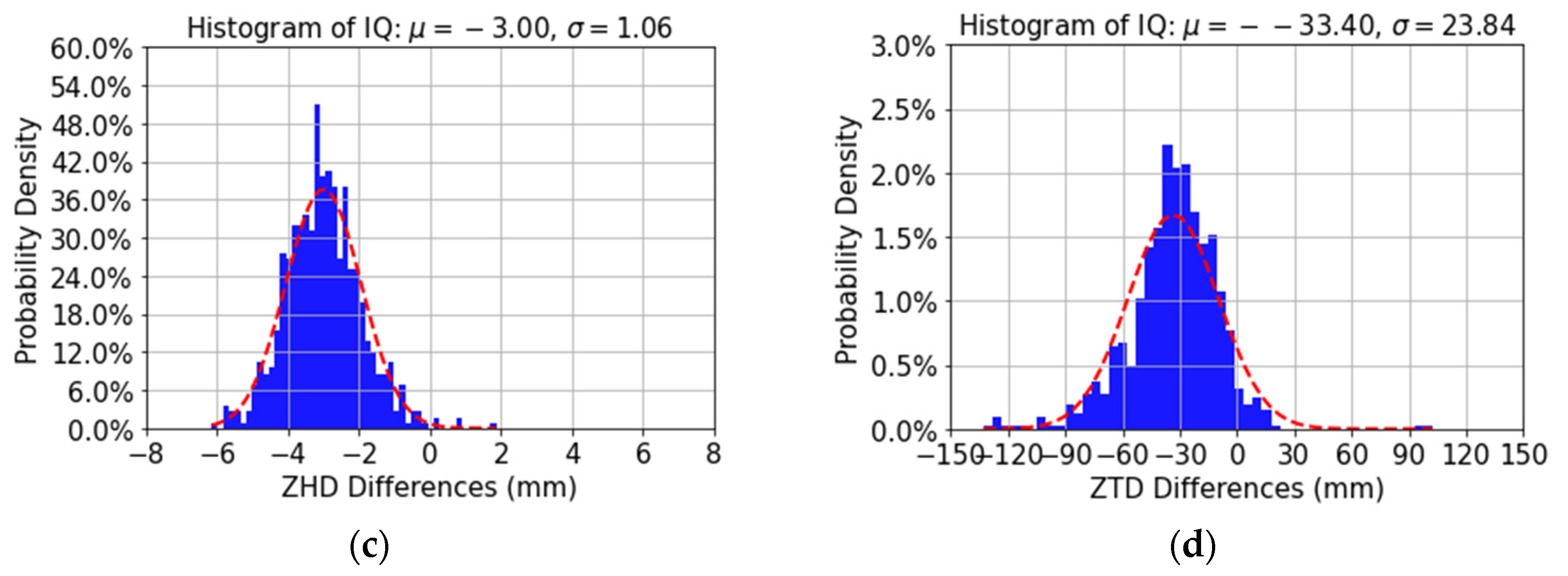
Figure 7a shows that the comparison of ZHD estimates based on Davis-Saastamoinen model [17] with ZHD estimates derived from RS and SA. The consistency is obvious, with a bias of −3.00 mm and an RMS of 3.18 mm (Table 7).
It is very well known that the zenith tropospheric delay (ZTD) effect on GNSS signals is defined as the sum of a hydrostatic part (ZHD) and a wet part (ZWD), as ZTD = ZHD + ZWD. To justify this equation in our case, we build for the FAA1 station, ZTD (RS + SA) = ZHD (RS + SA) + ZWD (RS). As already stated, nearly all the water vapor is concentrated in the troposphere, so there is no need to complement the computation of ZWD by considering a continuation in altitude by the standard atmosphere. We made a comparison between ZTD (RS + SA) and ZTD derived from GPS in Figure 7b. There is a large bias of about 33.40 mm and a large RMS of about 41.04 mm.
Given the fact that the ZWD from RS is reliable (see Section 4.4), this large bias points to a culprit on the GPS side, probably linked with a common cause shared by both our local processing and the IGS processing. The common cause could be (see Table 1), but is certainly not limited to, the PPP approach and the Earth tide models (solid and oceanic) [56,57]. Considering the orbital period of one-half a sidereal day (approximately 11h 58m) for GPS satellites [58], and semidiurnal periods of tide effects [59], we assume all of them have effects on ZWD estimates with a common period of around 12 h, which may lead to an unfortunate addition of these possible errors.

5. Discussion

Through above analysis of all elements, we think that the reason for the large systematic error showing up in the last step of the previous comparisons (ZTD estimation) is related to external sources in the GNSS processing. Possible causes, and certainly intertwined causes, could be orbits/clocks errors in the PPP corrections [49,51,60] and errors in the tide models (Earth tides, oceanic tides and loading models) [61,62,63]. It should be also noted that the THTI and FAA1 receivers used in this study are IGS stations belonging to the network of reference stations used in the PPP corrections [64] and that GNSS orbits and tides share a common periodicity of 12 h. From a physical point of view, the tides are showing up at two places: (1) their gravitational pull on the GNSS satellites; (2) the modulation in the receiver position. It is far beyond the scope of this paper, and of the practical resources of the authors, to pinpoint the exact cause(s) of the ZTD mismodeling in Tahiti, but the first idea that comes to mind is the remoteness of the Tahiti Island in the central South Pacific, with degraded accuracies in some underlying physical models for this specific location.

6. Conclusions

This paper was motivated by the results of a previous study [24] that pointed to overlarge values of the mean temperature of the troposphere for the tropical location of the Tahiti Island. To understand the reason(s) of these overestimations, we examined all the links of the computation chain leading to the mean temperature estimate. We first evaluated the accuracy of the ZTD estimates derived from our GPS data processing, based on a comparison with the CODE/IGS final products at two local IGS sites, FAA1 and THTI. We found that our ZTD estimates and CODE/IGS ZTD estimates are coherent at a millimeter level. Secondly, we compared the surface temperature measurements and estimates at FAA1 from a ground weather station, from the IGRA RS balloons launched from the same site and from the VMF1/ECMWF site-wise records. They all are coherent at the 1 K level. Thirdly, the weighted mean temperature of the atmosphere was estimated from the RS measurements (temperature and humidity) taken from the FAA1 balloon launch site and compared with the Tm values derived from the FAA1 site-wise VMF1/ECMWF records. We found that the Tm estimates from the RS data and the Tm estimates from VMF1/ECMWF are coherent within 0.56 K. This point also confirmed the underlying physical assumptions at the base of the Tm – Ts linear relationship. Fourthly, ZWD estimates were calculated by using the RS data at the FAA1 site and were compared with the corresponding ZWD values computed from the corresponding site-wise VMF1/ECMWF records. We found a large bias of 28.43 mm, indicating that the VMF1/ECMWF model is not a reliable source for estimating the water vapor contents of the troposphere, probably because its resolution in space and time is not enough to capture the high variability of water vapor at our scale. Fifthly, we calculated the ZHD estimates for the FAA1 site from the RS balloon data completed up to 100 km altitude by the U.S. Standard Atmosphere 1976 model. We found a bias of 3.00 mm and an RMS of 3.18 mm between these ZHD estimates and the ZHD estimates computed from the Saastamoinen model. Finally, we compared our ZTD (RS + SA) estimates with the ZTD estimates derived from our GPS data processing. We found a large bias of 33.40 mm associated with a large RMS of 41.04 mm.
If we take these elements together, we find that anomalous Tm values for the Tahiti Island are traced to anomalous ZTD, leading to an accuracy poorer by one order of magnitude than the claimed accuracy of ZTD delays from worldwide databases. The reason for the large systematic errors of these ZTD estimates is assumed to be related to external sources in the GNSS data processing. Although it is not practical to pinpoint the exact causes of the ZTD mismodelling in Tahiti, the first idea coming to mind is that the remote Tahiti Island in the central South Pacific may suffer from degraded accuracies in some underlying physical models for this specific location.

Author Contributions

Conceptualization, F.Z. conceived and performed the experiments under the supervision of J.-P.B.; F.Z., P.F., G.X. and J.-P.B. analyzed the data; F.Z. wrote the paper. All authors have read and agreed to the published version of the manuscript.

Funding

This research was funded by the National Natural Science Foundation of China (42274006, 42174035), the Open Fund of State Key Laboratory of Geodesy and Earth’s Dynamics (SKLGED2021-3-5), and a dedicated DAR Fund of the French Space Agency (CNES) for the Geodesy Observatory of Tahiti.

Data Availability Statement

The data presented in this study are available on request from the corresponding author.

Acknowledgments

We would like to thank the International GNSS Service (IGS) for giving raw GNSS data and tropospheric products, the Center for Orbit Determination in Europe (CODE) for providing the final products, the European Center for Medium-Range Weather Forecasts (ECMWF) for giving access to the VMF1 files, and the Integrated Global Radiosonde Archive (IGRA) for giving RS data.

Conflicts of Interest

The authors have no conflict of interest to declare.

Appendix A

The bias, RMS and STD, are used to quality the performances of the results with respect to the corresponding reference data. The formula is as follows [10]:
B i a s = 1 n i = 1 n ( G i R i ) ,
R M S = 1 n i = 1 n ( G i R i ) 2 ,
S T D = 1 n i = 1 n ( ( G i R i ) B i a s ) 2 ,
where i = 1, 2, 3,… n. n denotes the total number of data points. In this case, G denotes our results from GNSS data processing and R is the reference data.

References

  1. Zhang, F.; Barriot, J.-P.; Xu, G.; Hopuare, M. Modeling the Slant Wet Delays from One GPS Receiver as a Series Expansion with Respect to Time and Space: Theory and an Example of Application for the Tahiti Island. IEEE Trans. Geosci. Remote Sens. 2020, 58, 7520–7532. [Google Scholar] [CrossRef]
  2. Zhao, Q.; Liu, Y.; Ma, X.; Yao, W.; Yao, Y.; Li, X. An Improved Rainfall Forecasting Model Based on GNSS Observations. IEEE Trans. Geosci. Remote Sens. 2020, 58, 4891–4900. [Google Scholar] [CrossRef]
  3. Xia, P.; Xia, J.; Ye, S.; Xu, C. A new method for estimating tropospheric zenith wet-component delay of gnss signals from surface meteorology data. Remote Sens. 2020, 12, 3497. [Google Scholar] [CrossRef]
  4. Elliott, W.P.; Gaffen, D.J. On the Utility of Radiosonde Humidity Archives for Climate Studies. Bull. Am. Meteorol. Soc. 1991, 72, 1507–1520. [Google Scholar] [CrossRef]
  5. Liu, Y.; Liu, Y.; Chen, G.; Wu, Z. Evaluation of HY-2A satellite-borne water vapor radiometer with shipborne GPS and GLONASS observations over the Indian Ocean. GPS Solut. 2019, 23, 1–9. [Google Scholar] [CrossRef]
  6. Campmany, E.; Bech, J.; Rodríguez-Marcos, J.; Sola, Y.; Lorente, J. A comparison of total precipitable water measurements from radiosonde and sunphotometers. Atmos. Res. 2010, 97, 385–392. [Google Scholar] [CrossRef] [Green Version]
  7. Guo, J.; Hou, R.; Zhou, M.; Jin, X.; Li, G. Detection of particulate matter changes caused by 2020 california wildfires based on gnss and radiosonde station. Remote Sens. 2021, 13, 4557. [Google Scholar] [CrossRef]
  8. Zhang, S.; Fang, L.; Wang, G.; Li, W. The impact of second-order ionospheric delays on the ZWD estimation with GPS and BDS measurements. GPS Solut. 2020, 24, 1–11. [Google Scholar] [CrossRef]
  9. Lou, Y.; Huang, J.; Zhang, W.; Liang, H.; Zheng, F.; Liu, J. A new zenith tropospheric delay grid product for real-time PPP applications over China. Sensors 2018, 18, 65. [Google Scholar] [CrossRef] [PubMed] [Green Version]
  10. Zhang, F.; Barriot, J.-P.; Xu, G.; Hopuare, M. Analysis and Comparison of GPS Precipitable Water Estimates between Two Nearby Stations on Tahiti Island. Sensors 2019, 19, 5578. [Google Scholar] [CrossRef]
  11. Zhao, Q.; Liu, Y.; Yao, W.; Yao, Y. Hourly Rainfall Forecast Model Using Supervised Learning Algorithm. IEEE Trans. Geosci. Remote Sens. 2022, 60, 1–9. [Google Scholar] [CrossRef]
  12. Zhou, Y.; Lou, Y.; Zhang, W.; Wu, P.; Bai, J.; Zhang, Z. Tropospheric Second-Order Horizontal Gradient Modeling for GNSS PPP. Remote Sens. 2022, 14, 4807. [Google Scholar] [CrossRef]
  13. Zhang, H.; Yuan, Y.; Li, W. Real-time wide-area precise tropospheric corrections (WAPTCs) jointly using GNSS and NWP forecasts for China. J. Geod. 2022, 96, 1–18. [Google Scholar] [CrossRef]
  14. Hopfield, H.S. Tropospheric effect on electromagnetically measured range: Prediction from surface weather data. Radio Sci. 1971, 6, 357–367. [Google Scholar] [CrossRef]
  15. Saastamoinen, J. Contributions to the theory of atmospheric refraction. Bull. Géod. 1972, 105, 279–298. [Google Scholar] [CrossRef]
  16. Black, H.D. An Easily Implemented Range Correction for the Tropospheric Range Correction. Bull. Géod. 1978, 83, 1825–1828. [Google Scholar]
  17. Davis, J.L.; Herring, T.A.; Shapiro, I.I.; Rogers, A.E.E.; Elgered, G. Geodesy by radio interferometry: Effects of atmospheric modeling errors on estimates of baseline length. Radio Sci. 1985, 20, 1593–1607. [Google Scholar] [CrossRef]
  18. Huang, L.; Liu, L.; Chen, H.; Jiang, W. An improved atmospheric weighted mean temperature model and its impact on GNSS precipitable water vapor estimates for China. GPS Solut. 2019, 23, 51. [Google Scholar] [CrossRef]
  19. Bevis, M.; Businger, S.; Chiswell, S.; Herring, T.A.; Anthes, R.A.; Rocken, C.; Ware, R.H. GPS Meteorology: Mapping Zenith Wet Delays onto Precipitable Water. J. Appl. Meteorol. 1994, 33, 379–386. [Google Scholar] [CrossRef]
  20. Lu, C.; Li, X.; Zus, F.; Heinkelmann, R.; Dick, G.; Ge, M.; Wickert, J.; Schuh, H. Improving BeiDou real-time precise point positioning with numerical weather models. J. Geod. 2017, 91, 1019–1029. [Google Scholar] [CrossRef]
  21. Emardson, T.R.; Elgered, G.; Johansson, J.M. Three months of continuous monitoring of atmospheric water vapor with a network of Global Positioning System receivers. J. Geophys. Res. Atmos. 1998, 103, 1807–1820. [Google Scholar] [CrossRef]
  22. Suresh Raju, C.; Saha, K.; Thampi, B.V.; Parameswaran, K. Empirical model for mean temperature for Indian zone and estimation of precipitable water vapor from ground based GPS measurements. Ann. Geophys. 2007, 25, 1935–1948. [Google Scholar] [CrossRef] [Green Version]
  23. Mekik, C.; Deniz, I. Modelling and validation of the weighted mean temperature for Turkey. Meteorol. Appl. 2017, 24, 92–100. [Google Scholar] [CrossRef]
  24. Zhang, F.; Barriot, J.-P.; Xu, G.; Yeh, T.-K. Metrology Assessment of the Accuracy of Precipitable Water Vapor Estimates from GPS Data Acquisition in Tropical Areas: The Tahiti Case. Remote Sens. 2018, 10, 758. [Google Scholar] [CrossRef] [Green Version]
  25. Huang, L.; Wang, X.; Xiong, S.; Li, J.; Liu, L.; Mo, Z.; Fu, B.; He, H. High-precision GNSS PWV retrieval using dense GNSS sites and in-situ meteorological observations for the evaluation of MERRA-2 and ERA5 reanalysis products over China. Atmos. Res. 2022, 276, 106247. [Google Scholar] [CrossRef]
  26. Ross, R.J.; Rosenfeld, S. Estimating mean weighted temperature of the atmosphere for Global Positioning System applications. J. Geophys. Res. 1997, 102, 719–730. [Google Scholar] [CrossRef] [Green Version]
  27. Yao, Y.; Zhu, S.; Yue, S. A globally applicable, season-specific model for estimating the weighted mean temperature of the atmosphere. J. Geod. 2012, 86, 1125–1135. [Google Scholar] [CrossRef]
  28. Huang, L.; Jiang, W.; Liu, L.; Chen, H.; Ye, S. A new global grid model for the determination of atmospheric weighted mean temperature in GPS precipitable water vapor. J. Geod. 2019, 93, 159–176. [Google Scholar] [CrossRef]
  29. Bevis, M.; Businger, S.; Herring, T.A.; Rocken, C.; Anthes, R.A.; Ware, R.H. GPS meteorology: Remote sensing of atmospheric water vapor using the global positioning system. J. Geophys. Res. 1992, 97, 15787. [Google Scholar] [CrossRef]
  30. Thayer, G.D. An improved equation for the radio refractive index of air. Radio Sci. 1974, 9, 803–807. [Google Scholar] [CrossRef]
  31. Owens, J.C. Optical Refractive Index of Air: Dependence on Pressure, Temperature and Composition. Appl. Opt. 1967, 6, 51. [Google Scholar] [CrossRef]
  32. Bolton, D. The computation of equivalent potential temperature. Mon. Weather Rev. 1980, 108, 1046–1053. [Google Scholar] [CrossRef]
  33. Wang, X.; Zhang, K.; Wu, S.; Fan, S.; Cheng, Y. Water vapor- weighted mean temperature and its impact on the determination of precipitable water vapor and its linear trend. J. Geophys. Res. Atmos. 2016, 121, 833–852. [Google Scholar] [CrossRef]
  34. Barriot, J.-P.; Feng, P. Beyond Mapping Functions and Gradients. In Geodetic Sciences—Theory, Applications and Recent Developments; IntechOpen: London, UK, 2021. [Google Scholar]
  35. Askne, J.; Nordius, H. Estimation of tropospheric delay for microwaves from surface weather data. Radio Sci. 1987, 22, 379–386. [Google Scholar] [CrossRef]
  36. Serafini, J.; Barriot, J.-P.; Sichoix, L. The evolution of precipitable water and precipitation over the Island of Tahiti from hourly to seasonal periods. Int. J. Remote Sens. 2014, 35, 6687–6707. [Google Scholar] [CrossRef]
  37. Dach, R.; Lutz, S.; Walser, P.; Fridez, P. Bernese GNSS Software, Version 5.2; University of Bern, Bern Open Publishing: Bern, Switzerland, 2015; ISBN 9783906813059.
  38. Zhang, B.; Chen, Y.; Yuan, Y. PPP-RTK based on undifferenced and uncombined observations: Theoretical and practical aspects. J. Geod. 2019, 93, 1011–1024. [Google Scholar] [CrossRef]
  39. Boehm, J.; Werl, B.; Schuh, H. Troposphere mapping functions for GPS and very long baseline interferometry from European Centre for Medium-Range Weather Forecasts operational analysis data. J. Geophys. Res. Solid Earth 2006, 111, 1–9. [Google Scholar] [CrossRef]
  40. Kouba, J. A Guide to Using International GNSS Service (IGS) Products. Geod. Surv. Div. Nat. Resour. Canada Ottawa 2009, 6, 34. [Google Scholar]
  41. Ray, R.D.; Ponte, R.M. Barometric tides from ECMWF operational analyses. Ann. Geophys. 2003, 21, 1897–1910. [Google Scholar] [CrossRef] [Green Version]
  42. Durre, I.; Vose, R.S.; Wuertz, D.B. Overview of the integrated global radiosonde archive. J. Clim. 2006, 19, 53–68. [Google Scholar] [CrossRef] [Green Version]
  43. Feng, P.; Li, F.; Yan, J.; Zhang, F.; Barriot, J.P. Assessment of the accuracy of the saastamoinen model and vmf1/vmf3 mapping functions with respect to ray-tracing from radiosonde data in the framework of gnss meteorology. Remote Sens. 2020, 12, 3337. [Google Scholar] [CrossRef]
  44. Kouba, J. Implementation and testing of the gridded Vienna mapping function 1 (VMF1). J. Geod. 2008, 82, 193–205. [Google Scholar] [CrossRef]
  45. Vedel, H. Conversion of WGS84 Geogeometric Heights to NWP Model HIRLAM Geopotential Heights; Danish Meteorological Institute: Copenhagen, Danmark, 2000; pp. 1–16. [Google Scholar]
  46. U.S. Government. Standard Atmosphere; U.S. Government: Washington, DC, USA, 1976.
  47. Stull, R.B. Meteorology: For Scientists and Engineers; West Publishing: St. Paul, MN, USA, 1995. [Google Scholar]
  48. Abdelazeem, M.; El-Rabbany, A. Assessment of GNSS PPP-Based Zenith Tropospheric Delay. Artif. Satell. 2020, 55, 171–184. [Google Scholar] [CrossRef]
  49. Zumberge, J.F.; Heflin, M.B.; Jefferson, D.C.; Watkins, M.M.; Webb, F.H. Precise point positioning for the efficient and robust analysis of GPS data from large networks. J. Geophys. Res. Solid Earth 1997, 102, 5005–5017. [Google Scholar] [CrossRef] [Green Version]
  50. Labib, B.; Yan, J.; Barriot, J.P.; Zhang, F.; Feng, P. Monitoring Zenithal Total Delays over the three different climatic zones from IGS GPS final products: A comparison between the use of the VMF1 and GMF mapping functions. Geod. Geodyn. 2019, 10, 93–99. [Google Scholar] [CrossRef]
  51. Szołucha, M.; Kroszczyński, K.; Kiliszek, D. Accuracy of Precise Point Positioning (PPP) with the use of different International GNSS Service (IGS) products and stochastic modelling. Geod. Cartogr. 2018, 67, 207–238. [Google Scholar] [CrossRef]
  52. Jin, S.; Su, K. PPP models and performances from single- to quad-frequency BDS observations. Satell. Navig. 2020, 1, 1–13. [Google Scholar] [CrossRef]
  53. Mccarthy, P.W.; Liu, Z.; Cascioli, V. Humidity Sensors: Advances in Reliability, Calibration ans Application; MDPI: Basel, Switzerland, 2019; ISBN 9783039211234. [Google Scholar]
  54. Snajdrova, K.; Boehm, J.; Willis, P.; Haas, R.; Schuh, H. Multi-technique comparison of tropospheric zenith delays derived during the CONT02 campaign. J. Geod. 2006, 79, 613–623. [Google Scholar] [CrossRef]
  55. Zhang, D.; Guo, J.; Chen, M.; Shi, J.; Zhou, L. Quantitative assessment of meteorological and tropospheric Zenith Hydrostatic Delay models. Adv. Sp. Res. 2016, 58, 1033–1043. [Google Scholar] [CrossRef]
  56. Allinson, C.R.; Clarke, P.J.; Edwards, S.J.; King, M.A.; Baker, T.F.; Cruddace, P.R. Stability of direct GPS estimates of ocean tide loading. Geophys. Res. Lett. 2004, 31, 1–4. [Google Scholar] [CrossRef] [Green Version]
  57. Lyard, F.; Lefevre, F.; Letellier, T.; Francis, O. Modelling the global ocean tides: Modern insights from FES2004. Ocean Dyn. 2006, 56, 394–415. [Google Scholar] [CrossRef]
  58. Teunissen, P.J.G.; Montenbruck, O. Springer Handbook of Global Navigation Satellite System; Springer International Publishing: New York, NY, USA, 2017; ISBN 9783319429267. [Google Scholar]
  59. Kouba, J.; Héroux, P. Precise Point Positioning Using IGS Orbit and Clock Products. GPS Solut. 2001, 5, 12–28. [Google Scholar] [CrossRef]
  60. Zhang, B.; Hou, P.; Zha, J.; Liu, T. Integer-estimable FDMA model as an enabler of GLONASS PPP-RTK. J. Geod. 2021, 95, 91. [Google Scholar] [CrossRef]
  61. Melachroinos, S.A.; Biancale, R.; Llubes, M.; Perosanz, F.; Lyard, F.; Vergnolle, M.; Bouin, M.N.; Masson, F.; Nicolas, J.; Morel, L.; et al. Ocean tide loading (OTL) displacements from global and local grids: Comparisons to GPS estimates over the shelf of Brittany, France. J. Geod. 2008, 82, 357–371. [Google Scholar] [CrossRef]
  62. Boy, J.P.; Chao, B.F. Precise evaluation of atmospheric loading effects on Earth’s time-variable gravity field. J. Geophys. Res. Solid Earth 2005, 110, 1–10. [Google Scholar] [CrossRef] [Green Version]
  63. Francis, O.; Mazzega, P. Global charts of ocean tide loading effects. J. Geophys. Res. 1990, 95, 411–424. [Google Scholar] [CrossRef]
  64. Hackman, C.; Guerova, G.; Byram, S. International GNSS Service ( IGS ) Troposphere Products and Working Group Activities. In Proceedings of the from the Wisdom of the Ages to the Challenges of the Modern World Sofia, Sofia, Bulgaria, 17–21 May 2015; pp. 17–21. [Google Scholar]
Figure 1. Location of the THTI site (149.61°W, 17.58°S, ellipsoidal altitude 98.49 m) and FAA1 site (149.62°W, 17.56°S, ellipsoidal altitude 12.35 m) on Tahiti Island.
Remotesensing 14 05723 g001
Figure 2. Comparisons of our THTI ZTD estimates (cyan dots) with CODE/IGS THTI ZTD estimates (blue and red dots) (a), and FAA1 ZTD estimates (cyan dots), with CODE/IGS FAA1 ZTD estimates (blue and red dots) (b). See Table 2 for a statistical summary; (c) histograms of the ZTD differences between our THTI ZTD estimates and CODE/IGS THTI ZTD estimates; (d) histograms of the ZTD differences between our FAA1 ZTD estimates and CODE/IGS FAA1 ZTD estimates.
Remotesensing 14 05723 g002aRemotesensing 14 05723 g002b
Figure 3. FAA1 station: (a) comparison between the surface temperature from the ground weather station (T1, red dots) and from the site-wise VMF1/ECMWF files (T2, blue dots); (b) histograms of the temperature differences between the surface temperature from the ground weather station (T1) and from the site-wise VMF1/ECMWF files (T2).
Remotesensing 14 05723 g003
Figure 4. (a) FAA1 station: comparison between the RS − Tm values computed from Equation (14) (blue dots) and the VMF1/ECMWF − Tm values (red dots), and (b) histogram of the differences between the RS − Tm values and the VMF1/ECMWF − Tm values, and (c) linear fit between the RS − Tm and the VMF1/ECMWF – Ts, and (d) linear fit between the RS − Tm and the surface temperature measurements, Ts, from the FAA1 ground weather station.
Remotesensing 14 05723 g004aRemotesensing 14 05723 g004b
Figure 5. (a) FAA1 station: comparison between our RS-ZWD estimates (blue dots) with the ZWD estimates from VMF1/ECMWF (red dots); (b) histogram of the ZWD differences between the RS-ZWD values and the VMF1/ECMWF-ZWD values; (c) relationship between 1/Π (1/P1 for the y-axis, RS-ZWD/RS-PW) and 1/Tm (for the x-axis, RS − Tm), and their least-squares linear fit: 1/Π = 1779.61 ∗ 1/Tm − 0.07, with R2 = 99.78% (red line); (d) relationship between 1/Π (1/P2 for the y-axis, GPS-ZWD (VMF1/ECMWF)/RS-PW) and 1/Tm (for the x-axis, RS − Tm), and their least-squares linear fit: 1/Π = 5322.56 ∗ 1/Tm − 12.98, with R2 = 28.38% (red line).
Remotesensing 14 05723 g005
Figure 6. Comparisons of the new-SAAS ZHD estimates (green dots) and the old-SAAS ZHD estimates (blue dots) with the ZHD estimates from VMF1/ECMWF (red dots) for the FAA1 station (a), and the THTI station (b), and the histograms of their corresponding ZHD estimates differences at FAA1 station (c), and THTI station (d).
Remotesensing 14 05723 g006
Figure 7. FAA1 station: (a) Comparison of ZHD estimates (RS + SA, ZHD1) (black dots) with ZHD estimates based on the new Saastamoinen model (ZHD2) (red dots); (b) Comparison of ZTD (RS + SA, ZTD1) (green dots) with GPS ZTD estimates (ZTD2) (red dots); (c) histograms of the ZHD differences between SAAS ZHD estimates and ZHD (RS + SA) estimates; (d) histograms of the ZTD differences between GPS ZTD estimates and ZTD (RS + SA) estimates.
Remotesensing 14 05723 g007aRemotesensing 14 05723 g007b
Table 1. Data processing strategies of our ZTD estimates and IGS/CODE tropospheric products.
Our ZTD EstimatesIGSCODE
Precise satellite orbits and clocksCODE Final productsIGS Final productsCODE Final products
ApproachPPPPPPRelative positioning
Elevation angle cutoff3 degrees7 degrees3 degrees
Mapping functionVMF1 (Vienna Mapping Function 1)GMF (Global Mapping Function)VMF1
A priori troposphere estimateDry VMF modelDry Niell modelDry VMF model
Ionosphere correctionIonosphere-free linear combination of L1 and L2Ionosphere-free linear combination of L1 and L2Ionosphere-free linear combination of L1 and L2
Temporal resolution1 h5 min2 h
Ocean tidal loadingFES 2004FES 2004FES 2014b
Atmospheric tidal loadingRay and Ponte (2003) [41]Ray and Ponte (2003) [41]S1 + S2 tidal corrections from the Vienna atmospheric pressure model
Table 2. Statistical summary for the comparison between our THTI/FAA1 ZTD estimates and CODE/IGS THTI/FAA1 ZTD estimates (CODE/IGS values minus our ZTD values, Figure 2a,b) in terms of maximum (max), minimum (min), bias, root mean squares (RMS), and standard deviation (STD). The exact definitions of bias, RMS and STD, are shown in Appendix A.
DifferencesMax (mm)Min (mm)Bias (mm)RMS (mm)STD (mm)Data Points
THTICODE-our14.53−14.72−2.024.964.524244
IGS-our14.93−15.42−0.475.035.014244
FAA1CODE-our 22.89−23.39−0.517.067.044149
IGS-our26.36−26.711.098.158.084149
Table 3. Statistical summary for the comparisons (Figure 3) between the surface temperature from the ground weather station (T1) and from the site-wise VMF1/ECMWF files (T2) (T1 minus T2) in terms of max, min, bias, STD, and RMS.
DifferencesMax (K)Min (K)Bias (K)RMS (K)STD (K)Data Points
T1-T25.93−4.200.982.041.801458
Table 4. Statistical summary for the comparison between RS − Tm and Tm from VMF1/ECMWF (vmf1 minus RS) in terms of max, min, bias, STD and RMS.
DifferencesMax (K)Min (K)Bias (K)RMS (K)STD (K)Data Points
ECMWF—RS4.55−2.690.561.050.88724
Table 5. Statistical summary for the comparison between RS-ZWD and VMF1/ECMWF-ZWD (VMF1/ECMWF minus RS-ZWD) in terms of max, min, bias, STD, and RMS.
ZWD DifferencesMax (mm)Min (mm)Bias (mm)RMS (mm)STD (mm)Data
Points
VMF1-RS68.01−111.01−28.4336.5122.90724
Table 6. Statistical summary for the comparison between the new/old SAAS ZHD estimates and the VMF1/ECMWF ZHD estimates (VMF1/ECMWF minus new/old) in terms of max, min, bias, STD, and RMS, for Figure 6c,d.
DifferencesMax (mm)Min (mm)Bias (mm)RMS (mm)STD (mm)Data Points
ECMWF-old FAA14.08−4.68−0.591.301.161461
ECMWF-new FAA15.20−3.560.531.281.161461
ECMWF-old THTI4.18−4.60−0.481.261.161461
ECMWF-new THTI5.28−3.490.621.321.171461
Table 7. Statistical summary for Figure 7a,b for the comparison between ZHD1 and ZHD2 (ZHD2 minus ZHD1) and between ZTD1 and ZTD2 (ZTD2 minus ZTD1) in terms of max, min, bias, STD, and RMS.
DifferencesMax (mm)Min (mm)Bias (mm)RMS (mm)STD (mm)Data Points
ZHD2-ZHD11.87−6.14−3.003.181.06724
ZTD2-ZTD1102.61−132.97−33.4041.0423.84689
Publisher’s Note: MDPI stays neutral with regard to jurisdictional claims in published maps and institutional affiliations.

