Technical Note

A Multi-Band Atmospheric Correction Algorithm for Deriving Water Leaving Reflectances over Turbid Waters from VIIRS Data

1
Remote Sensing Division, Code 7232, Naval Research Laboratory, Washington, DC 20375, USA
2
Remote Sensing Division, Code 7234, Naval Research Laboratory, Washington, DC 20375, USA
*
Author to whom correspondence should be addressed.
Remote Sens. 2023, 15(2), 425; https://doi.org/10.3390/rs15020425
Submission received: 17 November 2022 / Revised: 6 January 2023 / Accepted: 8 January 2023 / Published: 10 January 2023
(This article belongs to the Special Issue Atmospheric Correction for Remotely Sensed Ocean Color Data)

Abstract

:
The current operational multi-band atmospheric correction algorithms implemented by NASA and NOAA for global remote sensing of ocean color from VIIRS (Visible Infrared Imaging Radiometer Suite) data are mostly based on the 2-band version of the SeaWiFS (Sea-Viewing Wide Field-of-View Sensor) algorithm. These algorithms generally use two NIR bands, one centered near 0.75 μm and the other near 0.865 μm, and a band ratio method for deriving aerosol information. The algorithms work quite well over open ocean waters. However, water leaving reflectances over turbid coastal waters are frequently not derived. We describe here a spectrum-matching algorithm using shortwave IR (SWIR) bands above 1 μm for retrieving water leaving reflectances in the visible from VIIRS data. The SWIR bands centered near 1.24, 1.61, and 2.25 μm are used in a spectrum-matching process to obtain spectral aerosol information, which is subsequently extrapolated to the visible region for the derivation of water leaving reflectances of visible bands. We present retrieval results for four VIIRS scenes acquired over turbid waters. We demonstrate that the spatial coverages of our retrieving results can be improved significantly in comparison with those retrieved with the current NOAA operational algorithm. If our SWIR algorithm is implemented for operational data processing, the algorithm can potentially be complimentary to current NASA and NOAA VIIRS algorithms over turbid waters to increase spatial coverages.

Graphical Abstract

1. Introduction

The US programs for multi-band remote sensing of ocean color from space has evolved from the past CZCS (Coastal Zone Color Scanner) [1], to SeaWiFS (Sea-Viewing Wide Field-Of-View Sensor) [2], to MODIS (Moderate Resolution Imaging Spectroradiometer) [3,4], and to the more recent VIIRS (Visible Infrared Imaging Radiometer Suite) [5]. Comprehensive reviews on the US satellite ocean color programs and evolution of atmospheric correction algorithms have recently been given by McClain et al. [6] and Gordon [7]. The algorithms were primarily designed for retrieving water leaving radiances in the visible over clear ocean areas (“Case 1” waters). The algorithms generally use two NIR bands, one centered near 0.75 μm and the other near 0.865 μm, and a band ratio method for deriving NIR aerosol information. The aerosol information in the visible is derived through extrapolation of the NIR information. In 1994, Gordon and Wang (GW94) [8] designed the SeaWiFS atmospheric correction algorithm. The MODIS and VIIRS atmospheric correction algorithms for ocean color applications are all based on the GW94 algorithm with minor deviations in actual code implementations. A complete description of the SeaWiFS algorithm was given by Mobley et al. [9]. At present, images of global VIIRS ocean color data products are routinely posted on a NASA ocean color web site (https://oceancolor.gsfc.nasa.gov (accessed on 7 January 2023)) and also on a NOAA ocean color web site (https://www.star.nesdis.noaa.gov/socd/mecb/color/ocview/ocview.html (accessed on 7 January 2023)). Based on our studying of these imaging data products, we have observed that ocean color products are routinely not retrieved over large portions of oceans, particularly over turbid coastal waters, with both the NASA and NOAA versions of VIIRS ocean color algorithms. In a recent investigation [10] on the interplay between ocean color data quality and quality, it has been found that the spatial coverage of the NOAA products is typically twice as large as those of the corresponding NASA products. Because the NOAA web site allows easy access to VIIRS imaging products, we use examples of NOAA VIIRS imaging products to illustrate the problems in this article. Our results will demonstrate that, despite the fact that the NOAA data products have better spatial coverage in comparison with the corresponding NASA data products, there is still room for improvement in the spatial coverage of NOAA products. This can be seen in the Figure 1 images described below.
Figure 1A shows a VIIRS global true color image (RGB) (R: 0.674-μm; G: 0.555-μm; B: 0.490-μm) for 14 September 2017. Figure 1B shows the same day VIIRS global chlorophyll-a image. Land surfaces were masked in grey color, while cloudy areas and extended sunglint-affected areas over water were masked in black color. The NOAA web site has a built-in image zooming capability. By looking at images over smaller geographic regions, problems associated with the VIIRS ocean color data products are revealed. Figure 1C shows the portion of the VIIRS RGB image in southern Florida and nearby waters. The silt induced by the strong winds of Hurricane Irma is seen. Bright and shallow water areas with reflection from the bottom around southern Florida and Bermuda areas are also seen. Figure 1D corresponds to Figure 1C, except for the Chl-a image. The silt feature seen in Figure 1C is not seen in Figure 1D. Most bright water pixels in the Figure 1C image were masked out in black color in Figure 1D. This indicates that the NOAA version of the VIIRS algorithm didn’t report retrievals over such bright water pixels. Figure 1E shows a portion of the VIIRS image covering portions of the eastern coastal area of China also acquired on 14 September 2017, while Figure 1F shows the Chl-a image over the same area. The colored turbid water areas in the left portion of Figure 1E were masked out in Figure 1F and no retrieval results were reported. For comparison, we show in Figure 1G a NASA quick-look global Chl-a image for the same day of 14 September 2017. Through visual inspections of Figure 1G with Figure 1B images, it is seen that more water areas were masked out in the NASA OC (Ocean Color) data product than those in the NOAA product. Until now, satellite ocean color missions have been focused on producing data products having the highest quality for climate research. The associated cost is not to do retrievals over large areas covered by turbid waters (see Figure 1B,G) as well as over very productive waters at high latitudes. The estimated suspended sediments as well as chlorophyll concentrations could potentially be biased lower over certain geographic regions.
The images in Figure 1 are just examples to demonstrate that the ocean color products are frequently not produced over large portions of water surfaces, especially over turbid waters, with the current NASA and NOAA versions of operational VIIRS ocean color algorithms. A study made by Feng and Hu [11] showed that, after eliminating poor quality OC data, the valid observations from the NASA Terra, or Aqua, MODIS instrument over global oceans were only approximately 5% on a daily basis.
In view of such non-retrieval issues, we have adapted a version of our previously developed hyperspectral atmospheric correction algorithm for deriving water leaving reflectances from multi-band VIIRS data. We describe in Section 2 the VIIRS’ spectral properties and our spectrum-matching technique using SWIR bands above 1 μm for deriving spectral aerosol information and for retrieving water leaving reflectances in the visible. We present in Section 3 sample results obtained from four sets of VIIRS data. We provide in Section 4 some discussions. In Section 5, we give conclusions.

2. Data and Methods

2.1. VIIRS Instrument

The VIIRS instrument is similar to the NASA Terra and Aqua MODIS instruments (Moderate Resolution Imaging Spectroradiometer) [3,4]. The names, positions, and widths of VIIRS bands below 2.5 μm are listed in Table 1. Many VIIRS bands (designated as M1 to M11) have heritages to MODIS but with minor differences in band positions and widths.
The positions and widths of these M-series of VIIRS bands are also shown in Figure 2. The bands are plotted over a reflectance spectrum acquired over a shallow water area with reflection from the sea floor. The bands below 1 μm (M1–M7) are illustrated in thick and short green bars. These bands are commonly referred to as visible and near-IR bands (VSNIR). Because the M7 band centered near 0.865 μm can receive solar light scattered by suspended sediments, this band is not ideally suited for retrieving aerosol information from satellite-measured data over turbid coastal waters. The four bands above 1 μm, i.e., M8, M9, M10, and M11, are marked in red color. These bands are referred to as shortwave IR bands (SWIR). Because liquid water absorption in the ocean above 1 μm is very strong, the water leaving reflectances of these SWIR bands in coastal waters are often close to zero. The M8, M10, and M11 bands are used in our VIIRS atmospheric correction algorithm. M9 is located inside an atmospheric water vapor band with strong absorption. It is now commonly used for thin cirrus detection from satellite images [12,13].

2.2. Atmospheric Corrections for VIIRS Data

In the late 1990s, we developed an ocean version of the hyperspectral atmospheric correction algorithm [14] for supporting the Navy COIS (Coastal Ocean Imaging Spectrometer) project [15]. Our algorithm was based on Robert Fraser’s radiative transfer formulation and algorithm [16,17]. The adoption of the Fraser formulation permits the simultaneous matching of measured radiances of several bands centered at different wavelengths with those from theoretical simulations and results in more stable estimates of aerosol models and optical depths.
In our hyperspectral algorithm, we convert radiances to reflectance units. We adopt the common definition of apparent reflectance ρ*obs at top-of-atmosphere (TOA) for a given wavelength as [14,18]
ρ*obs = π Lobs/(μo Eo)
where Lobs is the radiance of the ocean–atmosphere system measured by a satellite instrument, μo is the cosine of solar zenith angle, and Eo is the downward solar irradiance at TOA when the solar zenith angle is equal to zero. If we neglect the interactions between atmospheric gaseous absorption and molecular and aerosol scattering, we can express ρ*obs as [14,18]
ρ*obs = Tg [ρ*atm+sfc + ρw td tu/(1 − s ρw)],
where Tg is the total atmospheric gaseous transmittance on the Sun–surface–sensor path, ρ*atm+sfc is the reflectance resulted from scattering by the atmosphere and specular reflection by ocean surface facets, td is the downward transmittance (direct + diffuse), and tu is the upward transmittance, s is the spherical albedo that takes account of reflectance of the atmosphere for isotropic radiance incident at its base, and ρw is the water leaving reflectance.
Solving Equation (2) for ρw yields
ρw = (ρ*obs/Tg − ρ*atm+sfc)/[td tu + s (ρ*obs/Tg − ρ*atm+sfc)].
Given a satellite-measured radiance, the water leaving reflectance can be derived according to Equation (3) provided that the other quantities in the righthand side of Equation (3) can be modeled theoretically. We have used a modified version of the Ahmad and Fraser code [19] to generate lookup tables. More specifically, we use the code to generate the quantities ρ*atm+sfc, td, tu, and s in Equation (3). Lookup tables for 14 wavelengths between 0.39 and 2.5 μm in atmospheric “window” regions, sets of aerosol models, optical depths, solar and view angles, and surface wind speeds have been generated. Aerosol models similar to those used in the SeaWiFS algorithm, plus additional absorbing aerosol models, are used during the table generation.
It should be pointed out that the lookup tables used in the current generation of NASA, MODIS, and VIIRS algorithms were also generated with the Ahmad and Fraser code [19]. However, the NASA simulated tables (ρ*atm+sfc, td, tu, and s) were re-formatted in the form suitable for using the GW94 formulation to perform atmospheric corrections. For example, the term ρ*atm+sfc is separated into several terms, including a pure Rayleigh scattering term, a pure aerosol term, and a Rayleigh–aerosol interaction term. When aerosol optical depth is large or aerosols have absorption effects, such separations do not make too much scientific sense, although the GW94 formulation has been widely accepted by the ocean sciences research community.
In order to further verify the validity of our simulated lookup tables with the Ahmad and Fraser code, we also made numerous radiative transfer (RT) calculations with a recent vector radiative transfer code developed by Zhai and Hu [20]. We compared the simulation results with both algorithms for multiple solar zenith angles, view zenith angles, relative azimuth angles, aerosol models and optical depths, and surface wind speeds. The results from both algorithms typically agreed quite well (within the computing precision). For now, we are still using the lookup tables generated with the Ahmad and Fraser algorithm for modeling measured data that do not have bands below 0.39 μm. In the near future, we plan to use the tables generated with the Zhai and Hu RT algorithm because these tables have extended UV spectral coverage starting from 0.35 μm. These tables will be more useful for modeling the near future hyperspectral data to be collected with OCI (Ocean Color Instrument) from the NASA Plankton, Aerosol, and ocean Ecosystem (PACE) satellite mission.
In our hyperspectral atmospheric correction algorithm, we match the satellite-measured ‘apparent reflectances’ of selected SWIR bands with those pre-computed apparent reflectances for different aerosol models and optical depths. Our hyperspectral atmospheric correction algorithm has been tested with images acquired by a number of instruments, including the Airborne Visible Infrared Imaging Spectrometer (AVIRIS) [21] from an ER-2 aircraft at an altitude of 20 km. During the NASA-sponsored Sensor Intercomparison and Merger for Biological and Interdisciplinary Ocean Studies (SIMBIOS) program [22], we adapted the hyperspectral ocean atmospheric correction algorithm for processing multi-channel imagery, such as those acquired with the Terra and Aqua MODIS instruments. In our MODIS algorithm [23], both the MODIS land bands and ocean bands are used. This is necessary to overcome the MODIS ocean bands’ saturation problem over coastal waters. The lookup tables corresponding to MODIS wavelengths are obtained through linear interpolation of the tables generated for the hyperspectral atmospheric correction algorithm. The water leaving reflectances retrieved with our MODIS algorithm [23] over brighter and shallow coastal waters agreed well with those from field measurements. The NASA operational MODIS algorithm usually masked out the bright water pixels and made no retrievals over these pixels. This was partly due to the fact that the saturation radiances for some of the MODIS ocean color bands were not properly specified during the early planning stage of the MODIS instrument [4]. These bands were saturated over bright water pixels and not suitable for use in the derivation of ocean color data products. Our retrieved water leaving reflectances over deeper ocean waters compare well with those derived with the NASA MODIS operational algorithm, when both algorithms had retrieval results over the water surfaces.
With the experience gained in our development of a MODIS version of atmospheric correction, we have similarly developed a VIIRS ocean version of the atmospheric correction algorithm. The lookup tables corresponding to VIIRS wavelengths are obtained through linear interpolation of the tables generated for the hyperspectral atmospheric correction algorithm [14]. The module for modeling gas transmittance factors for VIIRS bands taking account of VIIRS bands’ properties are written separately. As a result, the atmospheric CO2 and CH4 absorption effect for the three VIIRS SWIR bands centered at 1.24, 1.61, and 2.25 μm is properly modeled. The three bands are typically used in our spectrum-matching algorithm for retrieving aerosol models and optical depths, and subsequently for the retrieval of water leaving reflectances in the visible.

3. Results

We have selected four turbid water scenes for deriving water leaving reflectances with our VIIRS version of the atmospheric correction algorithm. The four scenes were selected for different geographic regions. The first scene was acquired in southern Florida and nearby areas, after a major hurricane event. The second scene was over the eastern coastal area of China where the waters were quite turbid over extended areas. The third scene was over the Caspian Sea on a clear day. The fourth scene was off the eastern coastal area of Argentina when a chlorophyll blooming event occurred.

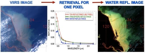
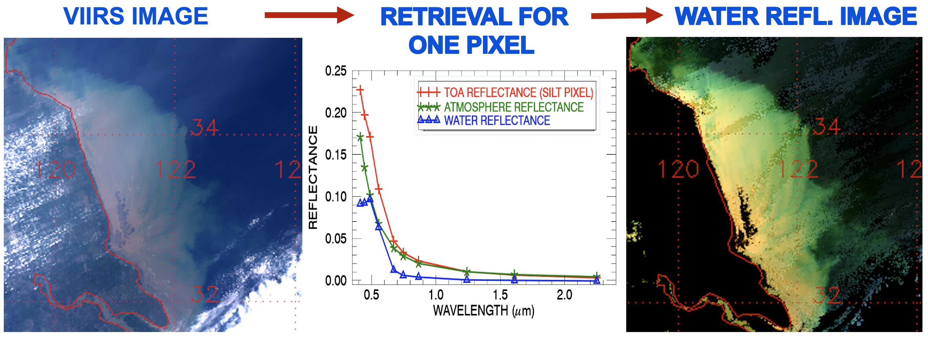
3.1. VIIRS Scene over Southern Florida Area, 14 September 2017

On September 14, 2017, over the coastal areas of Florida, large amounts of silt were stirred up by the strong winds of Hurricane Irma. Through visual inspection of VIIRS images and ocean color data products for the same day released publicly by NOAA (https://www.star.nesdis.noaa.gov/socd/mecb/color/ocview/ocview.html (accessed on 7 January 2023)), we found that VIIRS data over the Florida and Bermuda areas were captured under fairly clear sky conditions. As shown in Figure 1C, the wind-induced silt features as well as bright and shallow water areas having reflection from the ocean bottom surfaces are seen quite well. However, in the Figure 1D NOAA ocean color image, the silt features and large portions of bright water pixels were masked out. No ocean color data products were retrieved over these areas. We ordered the relevant VIIRS data sets (radiance and geolocation files) for the Florida scene from a NASA data center and made atmospheric corrections for the scene.
Figure 3A shows the RGB image we generated from the VIIRS data set. Figure 3B illustrates our spectrum-matching method for water leaving reflectance retrievals over a water pixel containing suspended silt particles. Figure 3B shows the apparent reflectances (the red line) for 10 VIIRS bands (the M9 band is not included). The estimation of spectral aerosol information is made from the 1.24-, 1.61-, and 2.25-μm bands by minimizing the sum of the squared differences between the measured data and calculated data using the spectrum-matching method. The aerosol information in the visible is then obtained through extrapolation. The estimated atmospheric reflectance, ρ*atm+sfc (as defined in Equation (2)), for the 10 VIIRS bands is shown as the green line in Figure 3B. According to Equation (3), the differences between the red line and the green line are proportional to water leaving reflectances. The blue line in Figure 3B showed the water leaving reflectances of VIIRS bands for the silt pixel. For the green band near 0.55-μm, the reflectance value is approximately 0.1, demonstrating that the suspended silt in the water is highly reflecting in the visible. This is consistent with what we see in the Figure 3A image. Figure 3C is the RGB image processed from our retrieved water surface reflectance data product. Clouds and land surface pixels were masked in black color. The elongated silt feature is seen obviously in this image. Water leaving reflectances over shallow and bright water pixels as well as over part of Lake Okeechobee, a large inland lake in southern Florida, are derived. Based on comparisons between the Figure 1D and 3C images, one can find that the area we made retrievals is more than double the area the NOAA algorithm made.

3.2. VIIRS Scene over Eastern Coastal Area of China, 14 September 2017

Waters in the eastern coastal region of China are frequently turbid. Satellite ocean color data products are often not derived. Here, we use the VIIRS data acquired over the region on 14 September 2017 as the second case for atmospheric corrections. Figure 4A shows a portion of VIIRS RGB image covering nearly the same area as that of Figure 1E. Figure 4B is the water leaving reflectance image retrieved with our algorithm. Land surfaces and bright clouds are masked in black color. By comparing this image with the Figure 1F image, it is seen that our algorithm is able to derive water leaving reflectances over brownish turbid water areas, while the NOAA operational VIIRS algorithm made no retrievals. A more quantitative comparison showed that the NOAA algorithm stopped retrievals over brownish water pixels with the M5 band (the red band) water leaving reflectance values of 0.03 or larger, while our algorithm was able to make retrievals over such turbid waters.

3.3. VIIRS Scene over Caspian Sea, 23 July 2022

Figure 5 shows the third case of ocean color retrievals from VIIRS data. Figure 5A is a color image covering the entire Caspian Sea area. The VIIRS scene was acquired on 23 July 2022 under fairly clear sky conditions. The image was obtained from the NOAA website. Figure 5B is the NOAA Chl-a image. In this image, land surfaces were masked in grey color, and water surfaces where no ocean color data product retrievals were made were masked in black color. By visual inspection of this image, it is seen that the NOAA ocean color algorithm made retrievals over only about half of water surfaces within and around the Caspian Sea. In view of the non-retrieval nature of the NOAA algorithm over bright water areas, we ordered the corresponding VIIRS radiance and geolocation data sets from a NASA data center and made atmospheric corrections with our algorithm. Figure 5C is the RGB image processed with our own computing system. Figure 5D is the RGB image processed from our retrieved water surface reflectance data product. Land and cloudy pixels are masked in black color in Figure 5D. Through comparisons between Figure 5C,D (or Figure 5A), one can see that our algorithm is able to make retrievals over most water pixels, including the bright water pixels in the upper, lower left, and lower right potions of the Caspian Sea. The area over which our algorithm made retrievals is roughly 70% larger than the area over which the NOAA algorithm made retrievals, based on visual comparisons between Figure 5B and D images.

3.4. VIIRS Scene off the Eastern Coastal Area of Argentina, 8 December 2017

Major chlorophyll blooming events often occur off the eastern coastal area of Argentina in December on a yearly basis. The spatial features associated with the blooming are easily captured by the MODIS and VIIRS satellite instruments. We selected a VIIRS chlorophyll blooming scene acquired off the eastern coastal area of Argentina on 8 December 2017 as the fourth case for water leaving reflectance retrievals. Figure 6A is an RGB image downloaded from the NOAA ocean color web site. Chlorophyll blooming features appear whitish in the left and lower right portion of this scene. Figure 6B showed the NOAA-posted Chl-a concentration image covering the same spatial area as that of Figure 6A. For reasons unknown to us, the spatial features in Figure 6B are not correlated with those in Figure 6A. We acquired the relevant VIIRS radiance and geolocation data sets from a NASA data center and processed the data. Figure 6C is our processed RGB image. Figure 6D is the RGB water leaving reflectance image processed from our retrieved surface reflectance data product. The chlorophyll features in Figure 6C all appear in Figure 6D—demonstrating the success of our algorithm in retrievals over the highly productive chlorophyll blooming waters.

4. Discussion

It should be pointed out that we are only able to make qualitative comparisons (based on visual inspections) of spatial coverages between our retrieval results and those from the NOAA operational algorithm. This is because, through the NOAA OCView website, we only acquired the images and not the original data that generated them. As a result, we did not have digital numbers to work with for quantifying differences in area coverages between our retrieval results and the results from the NOAA operational algorithm.
We feel that our VIIRS version of the atmospheric correction algorithm is already validated for the following reasons: The details on radiative transfer simulations [19], generation of lookup tables, and spectrum-matching processes were previously described in our hyperspectral ocean version of the atmospheric correction algorithm [12] and multi-channel MODIS algorithm [20]. The simulated lookup tables with the Ahmad and Fraser code is further verified with new lookup tables generated with a recent vector radiative transfer code (Zhai and Hu, 2022). The water leaving reflectance retrieving results from MODIS data were verified with measurements from a portable field spectrometer over surface stations in the Bahamas Banks and Florida Bay areas [20]. The results were also compared with those from the NASA operational MODIS algorithm. Because the lookup tables used in our VIIRS algorithm were obtained through interpolation of the same hyperspectral lookup tables simulated with the Ahmed and Fraser radiative transfer code [19], and because our hyperspectral and MODIS multi-spectral retrieving results were previously validated, we feel that it is not absolutely necessary to have additional validation of retrieval results for the few VIIRS cases presented here.

5. Conclusions

We have developed a spectrum-matching algorithm using shortwave IR (SWIR) bands above 1 μm for retrieving water leaving reflectances in the visible from VIIRS data. The SWIR bands centered near 1.24, 1.61, and 2.25 μm are used in a spectrum-matching process for estimating aerosol models and optical depths. The spectral aerosol information is extrapolated to the visible region for the derivation of water leaving reflectances of visible bands. We have demonstrated that the spatial coverages of our retrieving results are improved significantly in comparison with those retrieved with the current NOAA operational algorithm. If our SWIR algorithm is implemented for operational data processing, the algorithm can potentially be complementary to current NASA and NOAA VIIRS algorithms over turbid waters to increase spatial coverages.

Author Contributions

B.-C.G. originated the idea on the need to improve spatial area coverage in water leaving reflectance data products over turbid waters and developed the spectrum-matching algorithm for VIIRS retrievals. R.-R.L. performed retrievals and contributed to data analysis. All authors have read and agreed to the published version of the manuscript.

Funding

This research is supported by the US Office of Naval Research.

Data Availability Statement

All data are available on request.

Acknowledgments

The authors are grateful to Pengwang Zhai at the Physics Department, University of Maryland at Baltimore County for extensive calculations of lookup tables with his vector version of radiative transfer code, and to Menghua Wang with the Satellite Oceanography and Climatology Division of NOAA for pointing out the availability of a NOAA public web site (OCView) to view VIIRS RGB images and NOAA-retrieved ocean color product images.

Conflicts of Interest

The authors declare no conflict of interest.

References

  1. Gordon, H.R. Removal of atmospheric effects from satellite imagery of the oceans. Appl. Opt. 1978, 17, 1631–1636. [Google Scholar] [CrossRef] [PubMed]
  2. Hooker, S.B.; Esaias, W.E.; Feldman, G.C.; Gregg, W.W.; McClain, C.R. An overview of SeaWiFS and ocean color, NASA Goddard Space Flight Center, Greenbelt, MD. SewWiFS Tech. Rep. NASA Tech. Memo. 1992, 1, 104566. [Google Scholar]
  3. Salomonson, V.V.; Barnes, W.L.; Maymon, P.W.; Montgomery, H.E.; Ostrow, H. MODIS: Advanced facility instrument for studies of the earth as a system. IEEE Trans. Geosci. Remote Sens. 1989, 27, 145–153. [Google Scholar] [CrossRef]
  4. King, M.D.; Kaufman, Y.J.; Menzel, W.P.; Tanre, D. Remote sensing of cloud, aerosol, and water vapor properties from the Moderate Resolution Imaging Spectrometer (MODIS). IEEE Trans. Geosci. Remote Sens. 1992, 30, 2–27. [Google Scholar] [CrossRef] [Green Version]
  5. Murphy, R.E.; Barnes, W.L.; Lyapustin, A.; Privette, J.; Welsch, C.; DeLuccia, F.; Swenson, H.; Schueler, C.F.; Ardanuy, P.E.; Kealy, P.S.M. Using VIIRS to provide data continuity with MODIS. In Proceedings of the IEEE 2001 International Geoscience and Remote Sensing Symposium, Sydney, NSW, Australia, 9–13 July 2001; Available online: https://ieeexplore.ieee.org/stamp/stamp.jsp?tp=&arnumber=976795 (accessed on 7 January 2023).
  6. McClain, C.R.; Franz, B.A.; Werdell, P.J. Genesis and evolution of NASA’s satellite ocean color program. Front. Remote Sens. 2022, 3, 1–19. [Google Scholar] [CrossRef]
  7. Gordon, H.R. Evolution of ocean color atmospheric correction: 1970–2005. Remote Sens. 2021, 13, 5051. [Google Scholar] [CrossRef]
  8. Gordon, H.; Wang, M. Retrieval of water-leaving radiance and aerosol optical thickness over the oceans with SeaWiFS: A preliminary algorithm. Appl. Opt. 1994, 33, 443–452. [Google Scholar] [CrossRef] [PubMed]
  9. Mobley, C.D.; Werdell, J.; Franz, B.; Ahmad, Z.; Bailey, S. Atmospheric Correction for Satellite Ocean Color Radiometry; NASA T/M-2016-217551; NASA Goddard Space Flight Center: Greenbelt, Maryland, 2016; p. 73. [Google Scholar]
  10. Hu, C.; Barnes, B.; Feng, L.; Wang, M.; Jiang, L. On the interplay between ocean color data quality and data quantity: Impacts of quality control flags. IEEE Geosci. Rem. Sens. Lett. 2020, 17, 745–759. [Google Scholar] [CrossRef]
  11. Feng, L.; Hu, C. Comparison of valid ocean observations between MODIS Terra and Aqua over the global oceans. IEEE. Trans. Geosci. Remote Sens. 2016, 54, 1575–1585. [Google Scholar] [CrossRef]
  12. Gao, B.-C.; Kaufman, Y.J. Selection of the 1.375-µm MODIS channel for remote sensing of cirrus clouds and stratospheric aerosols from space. J. Atm. Sci. 1995, 52, 4231–4237. [Google Scholar] [CrossRef]
  13. Gao, B.-C.; Yang, P.; Han, W.; Li, R.-R.; Wiscombe, W.J. An algorithm using visible and 1.38-micron channels to retrieve cirrus cloud reflectances from aircraft and satellite data. IEEE Trans. Geosci. Remote Sens. 2002, 40, 1659–1668. [Google Scholar]
  14. Gao, B.-C.; Montes, M.J.; Ahmad, Z.; Davis, C.O. Atmospheric correction algorithm for hyperspectral remote sensing of ocean color from space. Appl. Opt. 2000, 39, 887–896. [Google Scholar] [CrossRef] [PubMed]
  15. Wilson, T.; Davis, C. Naval EarthMap Observer (NEMO) Satellite. 1999. Available online: https://www.spiedigitallibrary.org/conference-proceedings-of-spie/3753/0000/Naval-EarthMap-Observer-NEMO-satellite/10.1117/12.366268.pdf (accessed on 7 January 2023).
  16. Fraser, R.S.; Mattoo, S.; Yeh, E.-N.; McClain, C.R. Algorithm for atmospheric and glint corrections of satellite measurements of ocean pigment. J. Geophys. Res. 1997, 102, 17107–17118. [Google Scholar] [CrossRef] [Green Version]
  17. Fraser, R.; Ferrare, R.; Kaufman, Y.J.; Mattoo, S. Algorithm for atmospheric corrections of aircraft and satellite imagery. NASA Tech. Memo. 1989, 13, 100751. [Google Scholar] [CrossRef] [Green Version]
  18. Tanre, D.; Deroo, C.; Duhaut, P.; Herman, M.; Morcrette, J.J.; Perbos, J.; Deschamps, P.Y. Description of a computer code to simulate the satellite signal in the solar spectrum: The 5S code. Int. J. Remote Sens. 1990, 11, 659–668. [Google Scholar] [CrossRef]
  19. Ahmad, Z.; Fraser, R.S. An iterative radiative transfer code for ocean-atmosphere systems. J. Atmos. Sci. 1982, 39, 656–665. [Google Scholar] [CrossRef]
  20. Zhai, P.W.; Hu, Y. An improved pseudo spherical shell algorithm for vector radiative transfer. J. Quant. Spectr. Rad. Transf. 2022, 282, 108132. [Google Scholar] [CrossRef]
  21. Vane, G.; Green, R.O.; Chrien, T.G.; Enmark, H.T.; Hansen, E.G.; Porter, W.M. The Airborne Visible/Infrared Imaging Spectrometer. Remote Sens. Env. 1993, 44, 127–143. [Google Scholar] [CrossRef]
  22. McClain, C.; Esaias, W.; Feldman, G.; Frouin, R.; Gregg, W.; Hooker, S. The proposal for the NASA Sensor Intercalibration and Merger for Biological and Interdisciplinary Oceanic Studies (SIMBIOS) Program; NASA Tech. Memo. 2002-210008; NASA Goddard Space Flight Center: Greenbelt, Maryland, 2002; p. 54. [Google Scholar]
  23. Gao, B.-C.; Montes, M.J.; Li, R.-R.; Dierssen, H.M.; Davis, C.O. An atmospheric correction algorithm for remote sensing of bright coastal waters using MODIS land and ocean channels in the solar spectral region. IEEE Trans. Geosc. Remote Sens. 2007, 45, 1835–1843. [Google Scholar] [CrossRef]
Figure 1. (A) a NOAA global VIIRS RGB image for September 14, 2017; (B) same as (A), but for the NOAA global chlorophyll-a (Chl-a) image; (C) a portion of VIIRS RGB image around southern Florida and nearby waters; (D) same as (C), but for Chl-a image; (E) a portion of RGB image covering parts of turbid water areas in eastern coastal area of China; (F) same as (E), except for the Chl-a image, and (G) the NASA global Chl-a image for the same day.
Remotesensing 15 00425 g001
Figure 2. Bandpasses of VIIRS M bands in the 0.4–2.5 μm solar spectral range. A measured reflectance spectrum over a shallow water area having reflection from the bottom is also shown.
Remotesensing 15 00425 g002
Figure 3. (A)—a portion of VIIRS RGB image in southern Florida and nearby areas; (B)—spectral plots illustrating our spectrum-matching process; and (C)—the RGB image processed from our retrieved water leaving reflectance data.
Remotesensing 15 00425 g003
Figure 4. (A)—a portion of VIIRS RGB image acquired over the eastern coastal area of China on 14 September 2017; and (B)—the retrieved RGB water leaving reflectance image.
Remotesensing 15 00425 g004
Figure 5. (A)—a portion of NOAA-posted VIIRS RGB image over the Caspian Sea acquired on 23 July 2022; (B)—the NOAA-posted Chl-a image; (C)—the RGB image we obtained through processing the VIIRS radiance and geolocation data sets; and (D)—our retrieved RGB water leaving reflectance image.
Remotesensing 15 00425 g005
Figure 6. (A)—a portion of NOAA-posted VIIRS RGB image off the eastern coastal area of Argentina acquired on 8 December 2017; (B)—the NOAA-posted Chl-a image; (C)—the RGB image we obtained through processing the VIIRS radiance and geolocation data sets; and (D)—our retrieved RGB water leaving reflectance image. The spatial distribution patterns of chlorophyll blooming features are seen in (A,C,D).
Remotesensing 15 00425 g006
Table 1. The names, widths, and spatial resolution (m) of some VIIRS bands.
BandsWavelength (μm)Resolution (m)
M10.405–0.425750
M20.435–0.455750
M30.480–0.500750
M40.545–0.565750
M50.663–0.684750
M60.736–0.756750
M70.846–0.885750
M81.230–1.250750
M9 (Cirrus Band)1.368–1.388750
M101.580–1.640750
M112.225–2.275750
Disclaimer/Publisher’s Note: The statements, opinions and data contained in all publications are solely those of the individual author(s) and contributor(s) and not of MDPI and/or the editor(s). MDPI and/or the editor(s) disclaim responsibility for any injury to people or property resulting from any ideas, methods, instructions or products referred to in the content.

