Article

Hyper-LGNet: Coupling Local and Global Features for Hyperspectral Image Classification

1
School of Automation and Electrical Engineering, University of Science and Technology Beijing, Beijing 100083, China
2
Key Laboratory of Knowledge Automation for Industrial Processes, Ministry of Education, Beijing 100083, China
3
Shunde Innovation School, University of Science and Technology Beijing, Foshan 528000, China
*
Author to whom correspondence should be addressed.
Remote Sens. 2022, 14(20), 5251; https://doi.org/10.3390/rs14205251
Submission received: 30 August 2022 / Revised: 7 October 2022 / Accepted: 18 October 2022 / Published: 20 October 2022

Abstract

:
Hyperspectral sensors provide an opportunity to capture the intensity of high spatial/spectral information and enable applications for high-level earth observation missions, such as accurate land cover mapping and target/object detection. Currently, convolutional neural networks (CNNs) are good at coping with hyperspectral image processing tasks because of the strong spatial and spectral feature extraction ability brought by hierarchical structures, but the convolution operation in CNNs is limited to local feature extraction in both dimensions. In the meanwhile, the introduction of the Transformer structure has provided an opportunity to capture long-distance dependencies between tokens from a global perspective; however, Transformer-based methods have a restricted ability to extract local information because they have no inductive bias, as CNNs do. To make full use of these two methods’ advantages in hyperspectral image processing, a dual-flow architecture named Hyper-LGNet to couple local and global features is firstly proposed by integrating CNN and Transformer branches to deal with HSI spatial-spectral information. In particular, a spatial-spectral feature fusion module (SSFFM) is designed to maximally integrate spectral and spatial information. Three mainstream hyperspectral datasets (Indian Pines, Pavia University and Houston 2013) are utilized to evaluate the proposed method’s performance. Comparative results show that the proposed Hyper-LGNet achieves state-of-the-art performance in comparison with the other nine approaches concerning overall accuracy (OA), average accuracy (AA) and kappa index. Consequently, it is anticipated that, by coupling CNN and Transformer structures, this study can provide novel insights into hyperspectral image analysis.

Graphical Abstract

1. Introduction

With the development of sensing technology, hyperspectral sensors provide an opportunity to realize the acquisition of hundreds of bands for each pixel, capturing the intensity of the reflectance of high spatial/spectral information and enabling the detection of various objects [1,2,3]. In comparison with red-green-blue (RGB)-based sensing images and multispectral images (MSI), hyperspectral images (HSI) contain hundreds of pieces of spectrum band information because of the increasing band and decreasing bandwidth of each spectral band [4]. Such abundant band information has a more powerful discriminating ability, especially for similar spectral categories, and thus has been widely applied in high-level earth observation (EO) missions, such as accurate land cover mapping, precision agriculture, target/object detection, urban planning, mineral exploration, and so on [5,6,7].
The land cover mapping problem in high-level Earth observation missions can be transformed as an image classification problem, aiming to identify various objects so that vital information can be obtained by key stakeholders for decision making [8,9,10]. In the early stage, the solution to cope with the HSI classification problem by traditional approaches with feature extraction methods was proposed and applied, including via machine learning methods, such as random forest (RF) [11], k-nearest neighbors (k-NNs) [12], support-vector machines (SVMs) [13], K-means [14], and so on. However, these conventional classification methods require human experience for feature extraction, thus resulting in a poor performance. In recent years, the appearance of deep learning methods has enhanced the ability to analyze hyperspectral images with an accurate and robust approach, including via convolutional neural networks (CNNs), recurrent neural networks (RNNs), and so on [5,15,16]. Conventional machine learning techniques require careful engineering and considerable domain expertise to design a feature extractor transforming the raw HSI data [17]. In contrast, deep learning methods can strongly extract the representations of raw data that are needed for HSI classification [18,19]. Until now, many novel algorithms have achieved great performance in HSI classification. Swalpa et al. proposed a new end-to-end morphological framework to model nonlinear information during the training process, achieving superior performance in contrast with traditional CNNs on the Indian Pines and Pavia University datasets [20]. Focusing on multi-modal remote sensing data classification, Wu et al. designed a reconstruction strategy called CCR-Net to learn more compact fusion representations of RS data sources, demonstrating its effectiveness on the Houston 2013 dataset [21]. Sellami et al. proposed a novel methodology based on multi-view deep neural networks [
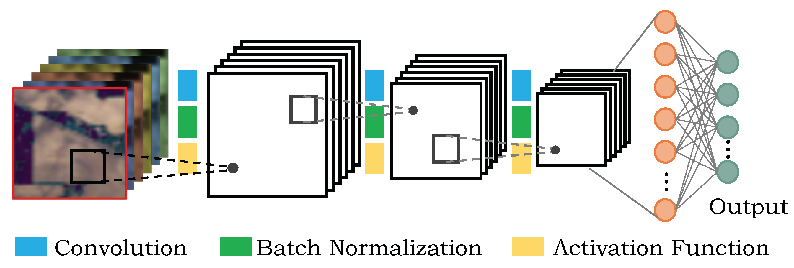
22]. In this method, images are initial processed and a specially designed autoencoder and semi-supervised networks are adopted to reach SOTA results on the Indian Pines, Salinas, and Pavia University datasets. Among these deep learning-based methods, CNNs have attracted many scholars to use them on hyperspectral image analysis for spatial and spectral feature extraction due to the strong feature extraction ability of the convolution operation and the strong representation ability brought by their hierarchical structure [23,24].
According to the form of input data, CNN-based methods for HSI classification can be divided into spectral CNNs, spatial CNNs, and spectral-spatial CNNs. Spectral CNNs take the pixel vector as input and utilize CNNs to accomplish the classification task only in the spectral dimension. For example, Hu et al. proposed a 1D CNN with five stacked convolutional layers to extract the spectral features of HSI [25]. Furthermore, Li et al. proposed a novel CNN-based method to encode pixel-pair features and made prediction results via a voting strategy, obtaining excellent classification performance [26]. To fully exploit the rich spatial information, spatial CNN-based methods were proposed to extract the spatial features of HSI. For example, Haut et al. proposed to use cropped image patches with centered neighboring pixels to train 2D CNNs for HSI classification instead of only a pixel in the previous way [27]. Xu et al. proposed RPNet to combine both shallow and deep convolutional features, creating a better adaption to the multi-scale object classification of HSI [28]. Since spectral and spatial information are both crucial for the accurate classification of HSI, spectral-spatial CNN-based methods have been further proposed for jointly exploiting spectral and spatial features in HSI [29]. For instance, Zhong et al. proposed to use 3D convolutional layers to extract spectral-spatial information with batch normalization regularizing the model [30]. He et al. proposed a deep 3D CNN to jointly learn both 2D multi-scale spatial features and 1D spectral features from HSI data in an end-to-end approach, achieving state-of-the-art results on the standard HSI datasets [31].
However, although CNN-based feature extractors have achieved great results in hyperspectral image analysis by employing spatial and spectral information according to the aforementioned reviews, some particular characteristics of CNNs may restrict the network’s performance on the HSI classification problem. The convolution operation in the CNN method is only limited to local feature extraction, whether in the spectral dimension or the spatial dimension; therefore, the receptive field can only be further increased by stacking the number of layers. As a consequence, such a process is often unable to effectively obtain the global receptive field and leads to a huge computation load due to the increase in model parameters. As a result, the CNN-based method is always applied in HSI classification with other strategies to achieve better performance, such as with multiscale dynamic graph and hashing semantic features [32,33].
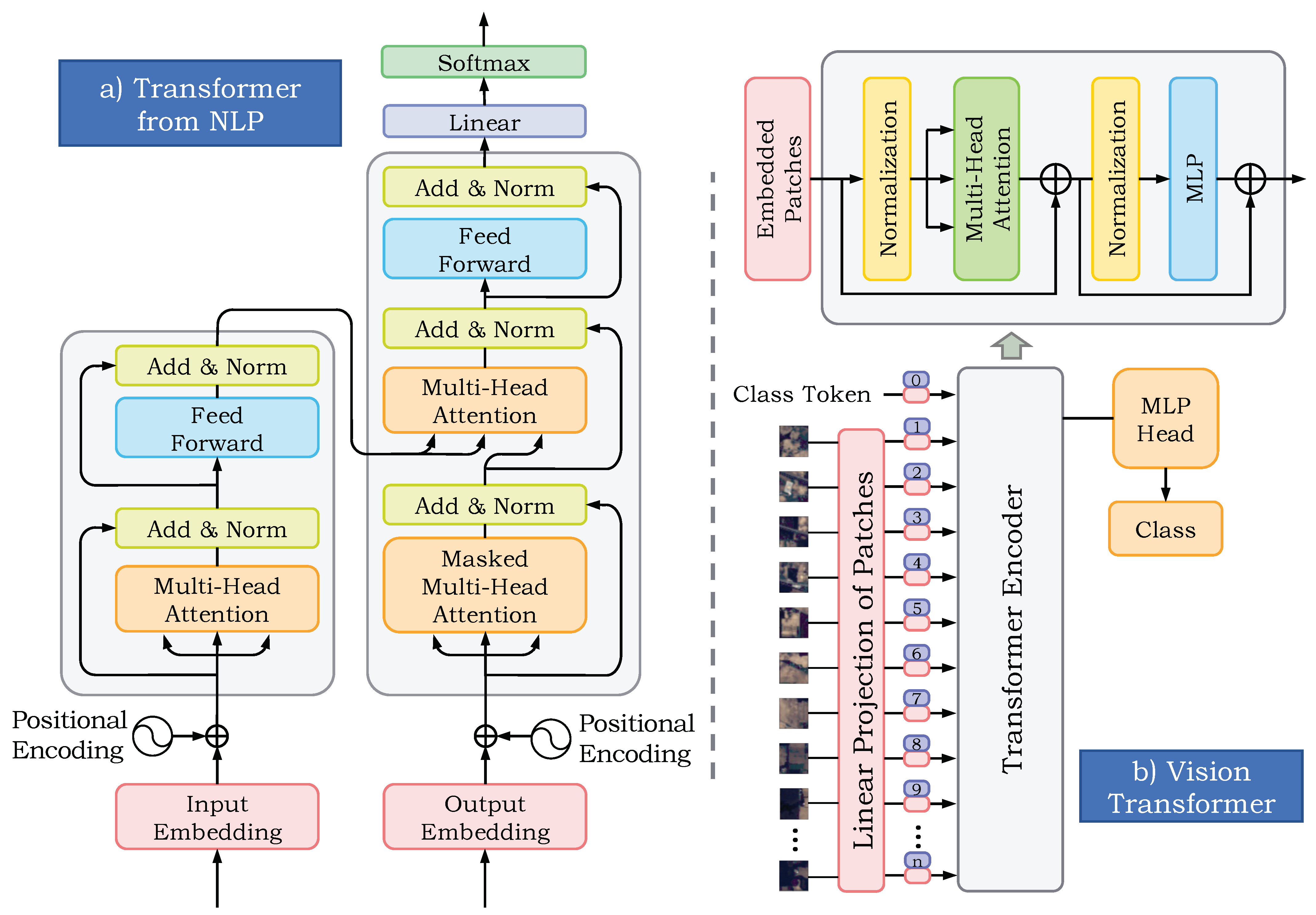
To overcome the drawbacks brought by CNNs, the Transformer structure is designed for processing and analysing sequential data, particularly in image analysis problems. Because of its unique internal multi-head self-attention mechanism, Transformer is capable of capturing long-distance dependencies between tokens from a global perspective. Inspired by related reviews, Transformer has achieved quite good results on multiple downstream tasks in the natural language processing (NLP) and computer vision (CV) domains with the help of large-scale pre-training [34,35,36]. Furthermore, Transformer has also achieved superior results in the field of hyperspectral image classification. For example, to solve the limited receptive field, inflexibility and difficult generalization problems, HSI-BERT was proposed to capture the global dependence among spatial pixels with bidirectional encoder representations from Transformers [37]. Spatial-spectral Transformer utilized a CNN to extract the spatial features and a modified Transformer to capture global relationships in the spectral dimension, fully exploring the spatial-spectral features [38]. Moreover, the spatial Transformer network was proposed to obtain the optimal input of HSI classifiers for the first time [39]. Rethinking hyperspectral image classification with Transformers, SpectralFormer can learn spectral local information from neighboring bands of HS images, achieving a significant improvement in comparison with state-of-the-art backbone networks [7].
It should be emphasized that although a single Transformer network can pave the way for the HSI classification problem compared to CNN methods by the means of both spatial and spectral information, it still has some problems. First, the Transformer method has a restricted ability to extract local information since it does not possess the strong inductive bias that CNNs do. Second, Transformer needs large-scale pre-training to achieve the same performance as a CNN. Third, the computation load is strongly positive and correlated to the sequence length, so that the Transformer-based method will be unduly computationally intensive when the sequence length is excessively long, and the Transformer’s representational ability will also be limited if the sequence length is too short. Therefore, an adequate approach to combine the benefits of each paradigm (CNN-based and Transformer-based methods) applying spatial and spectral information in the field of the HSI classification task is a challenging problem.
Currently, many scholars attribute their work in the HSI classification problem, including traditional machine learning methods, CNN-based approaches and Transformer-based methods. Although some works integrate CNN and Transformer via a hybrid strategy in a single branch, the spatial and spectral information of HSI are not fully fused and utilized. Local features and global features are not complementary at the receptive field level, and the features of only one branch cannot help the model to discriminate various classes through a feature fusion method, resulting in a less convincing and accurate classification performance [
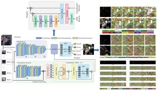
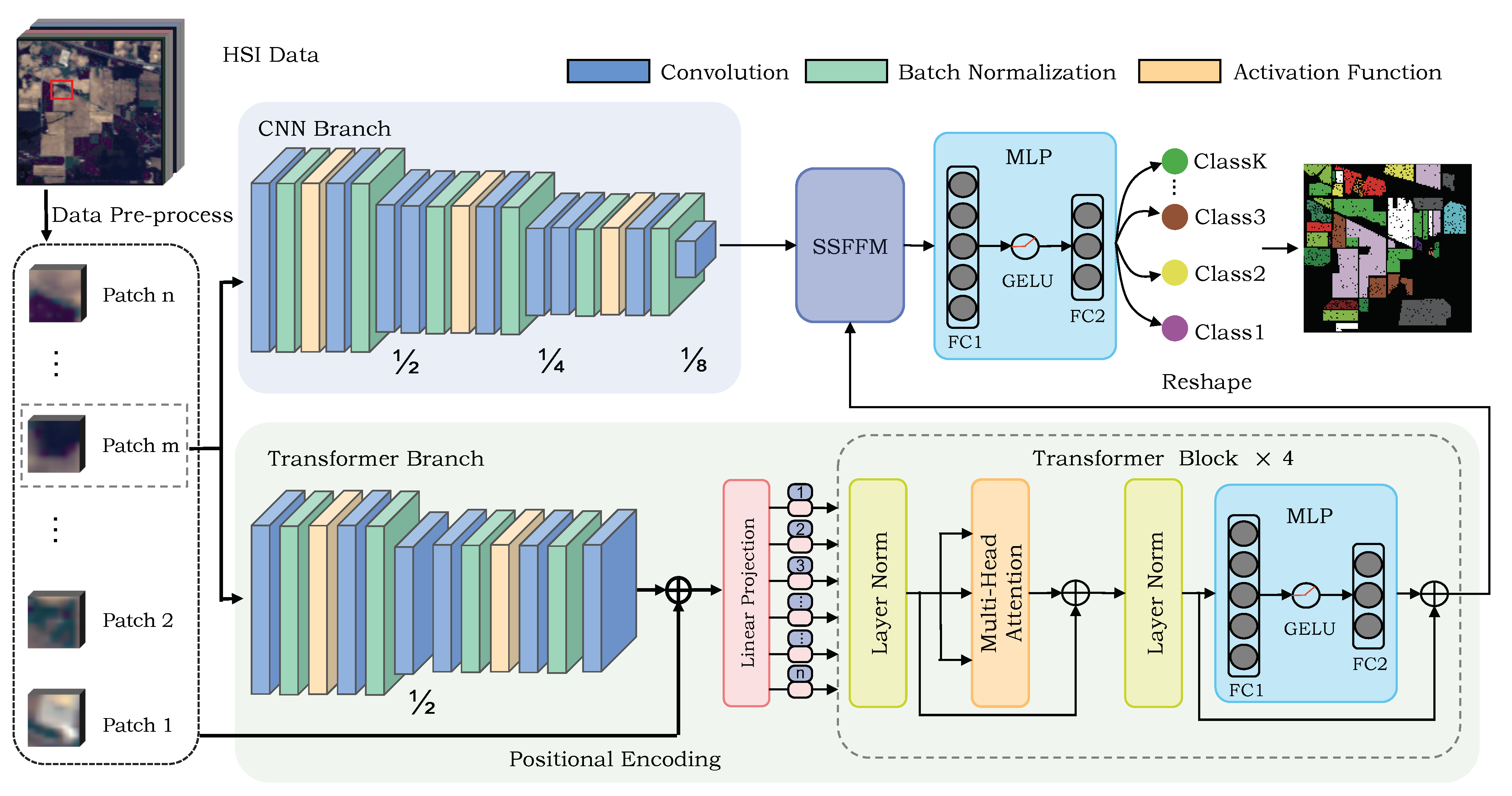
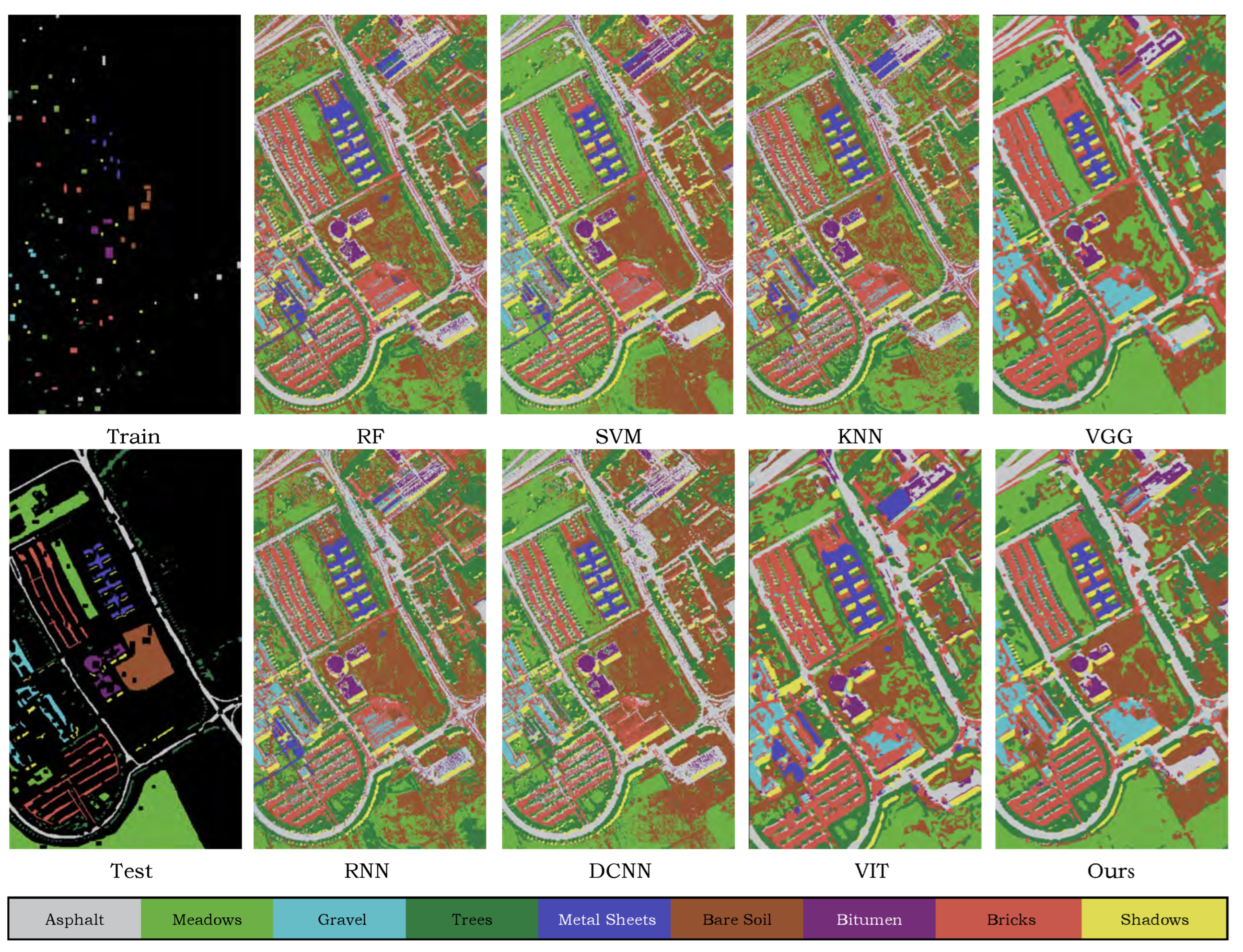
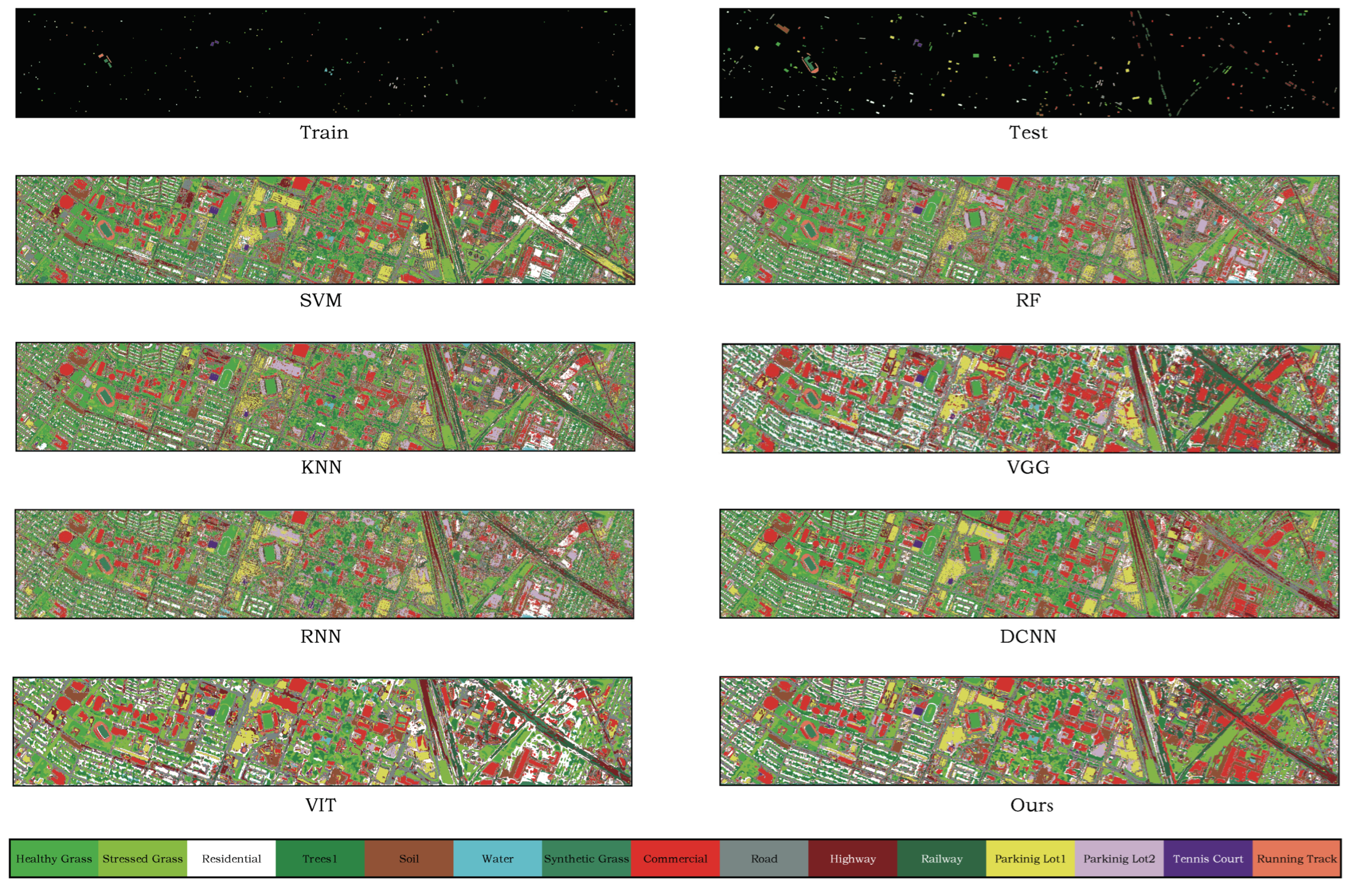
39]. To address these previous drawbacks introduced by a single CNN and Transformer network, the dual flow framework named Hyper-LGNet aiming to couple local and global features for hyperspectral image classification is proposed, using CNN and Transformer branches to deal with HSI spatial-spectral information. The proposed Spatial-spectral Feature Fusion Module (SSFFM) is applied to integrate spectral and spatial information maximally. The proposed method is validated by using three popular datasets: the Indian Pines, Pavia University and Houston 2013 datasets. The results are compared with traditional machine learning methods and other deep learning architectures, showing that our result achieves the best performance among others even compared with previous SOTA SpectralFormer [7]. To be more clear, the main contributions are summarized as follows:
(1)
A dual flow architecture named Hyper-LGNet is proposed, which utilizes CNN and Transformer models from two branches to obtain HSI spatial and spectral information for HSI classification problems on the first attempt.
(2)
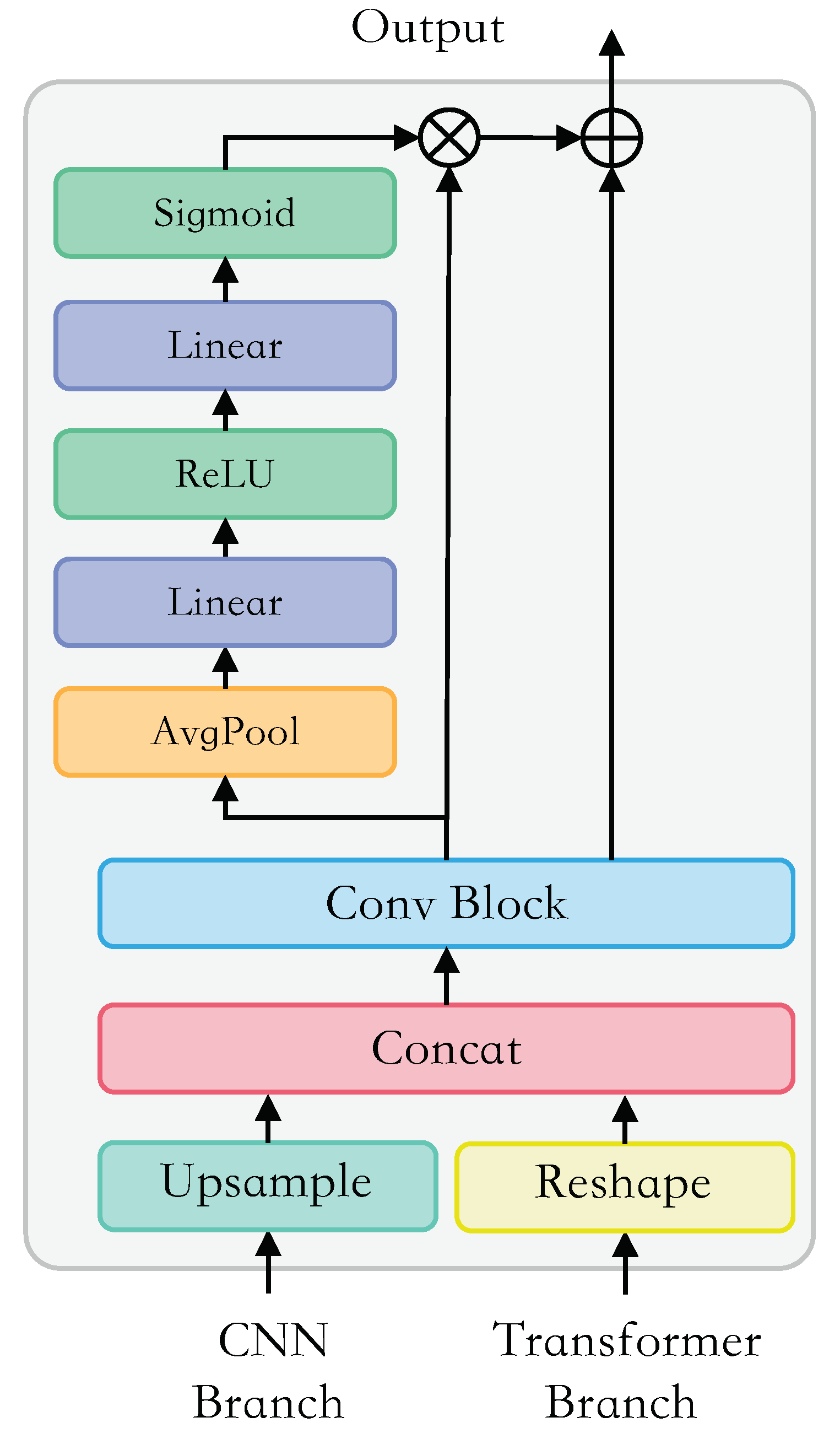
The sensing image feature fusion block, namely the Spatial-spectral Feature Fusion Module, is proposed to maximally fuse spectral information and spatial information from two branches in a dual-flow architecture.
(3)
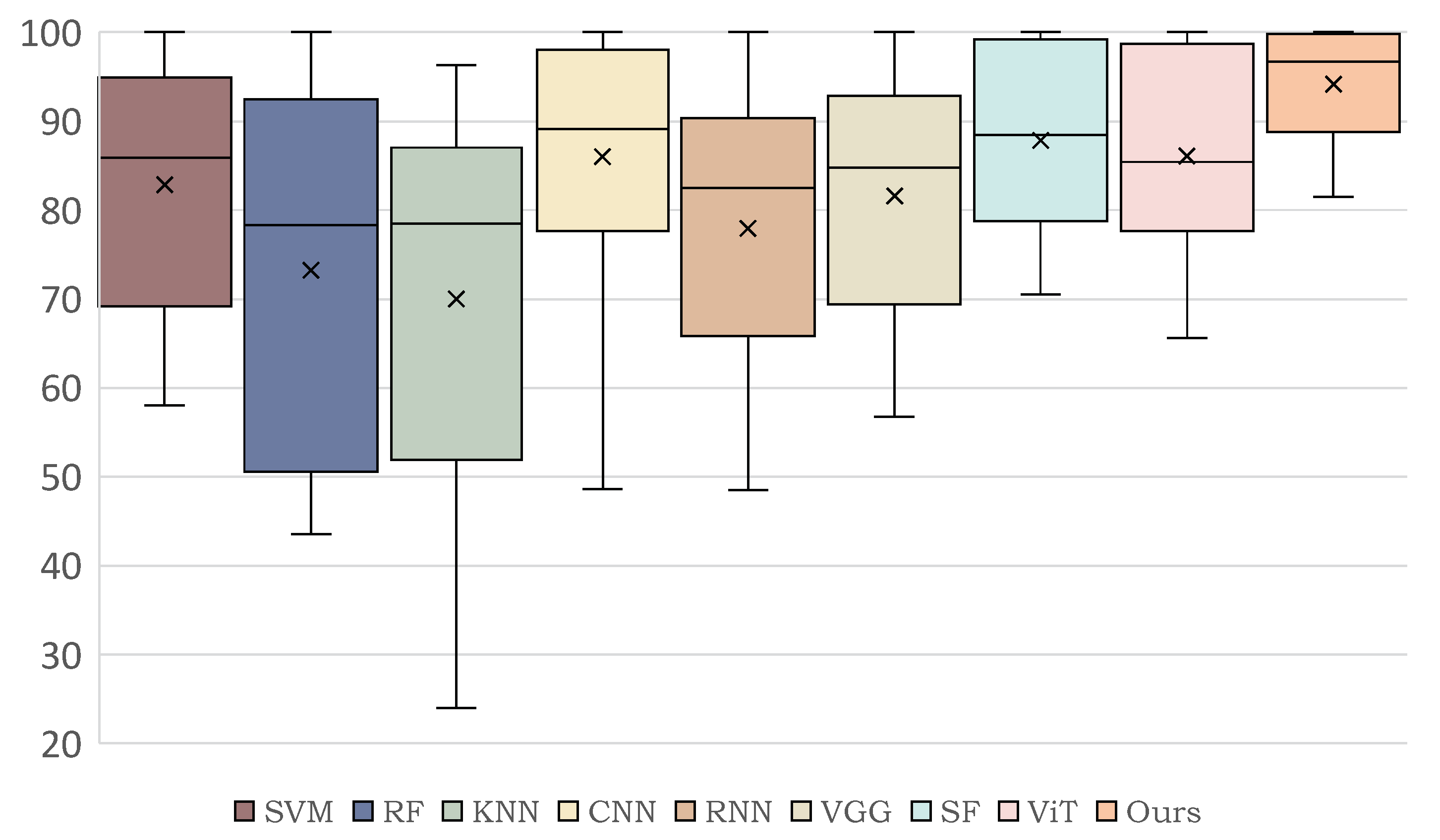
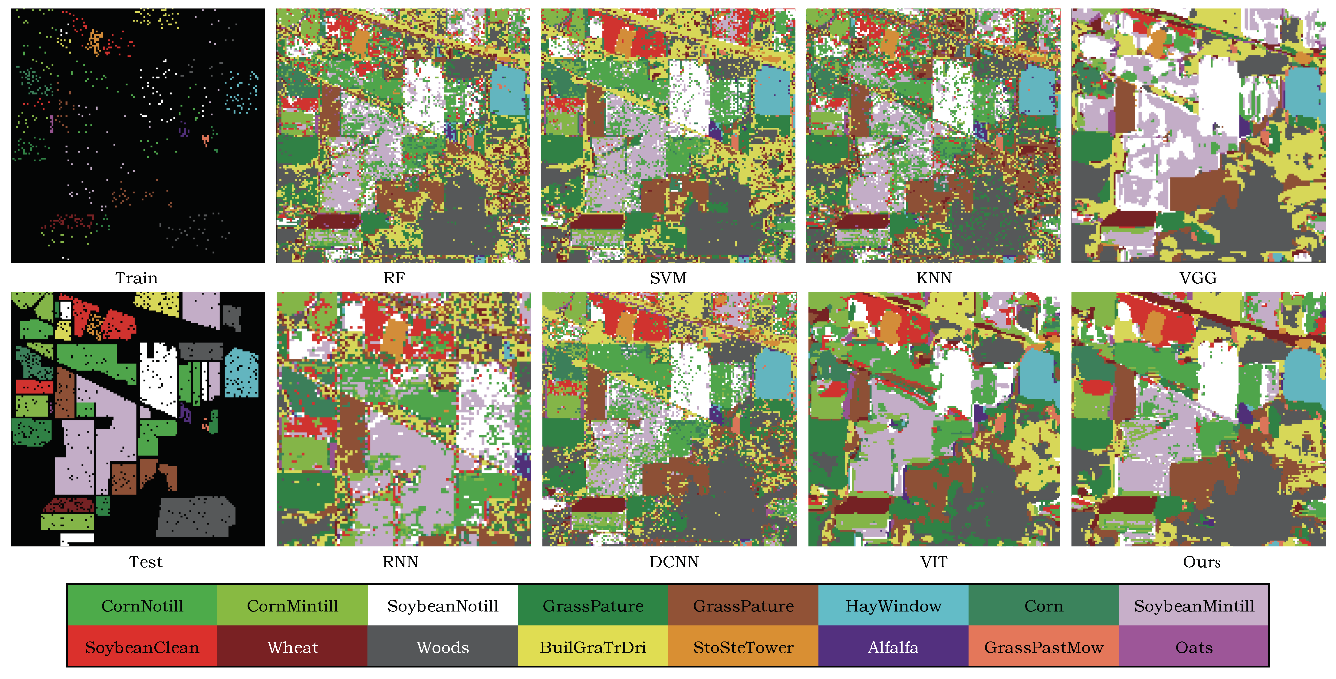
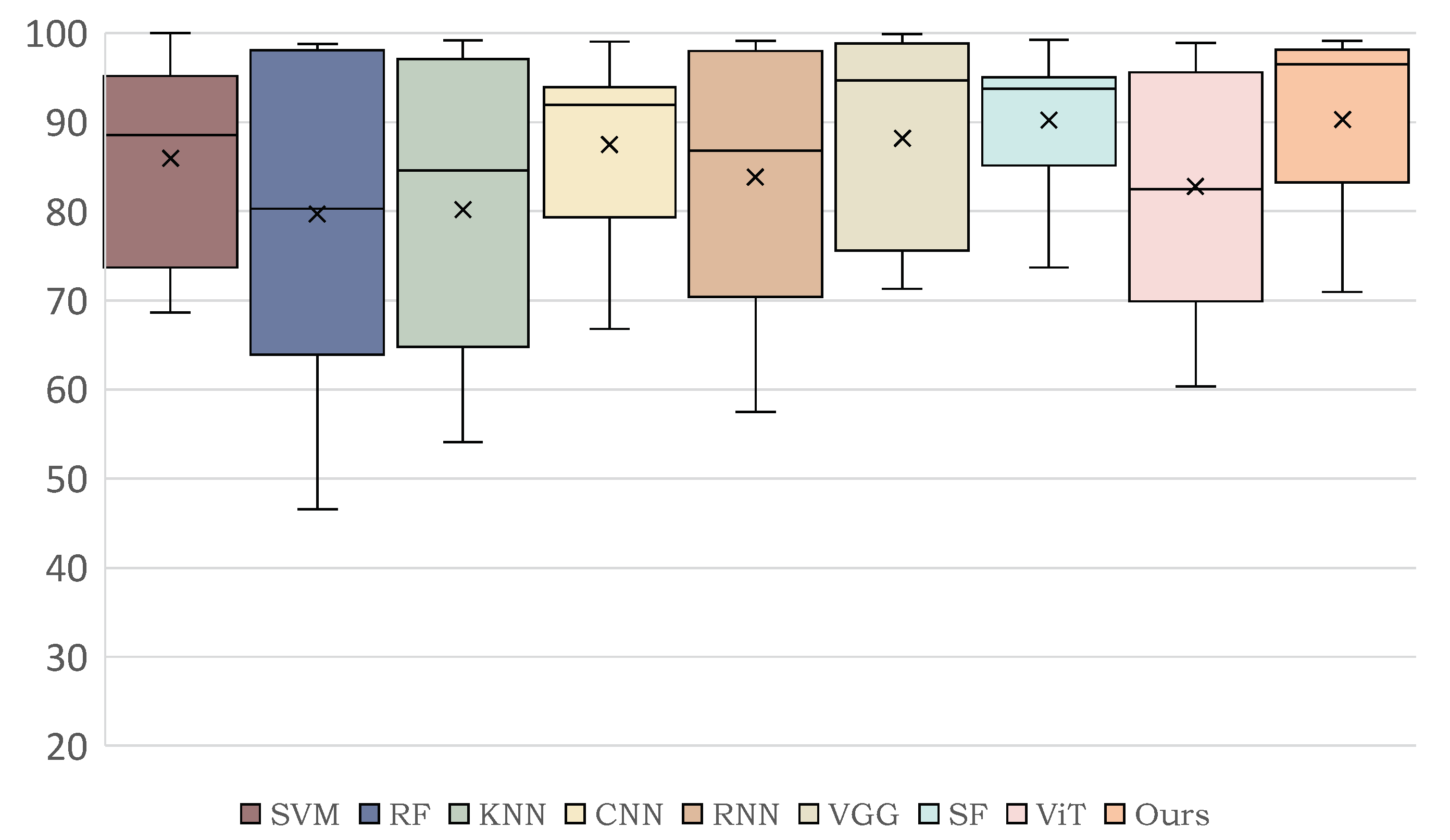
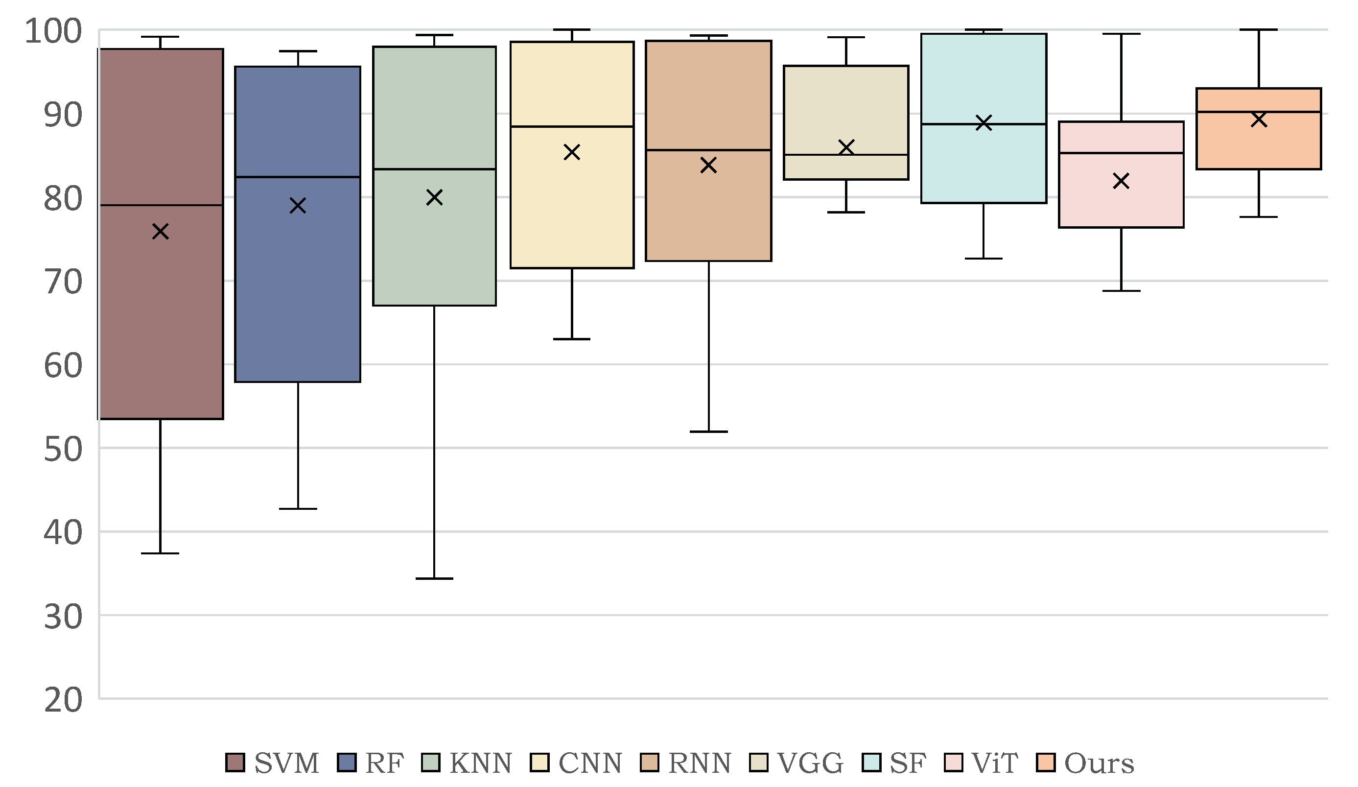
Extensive experiments are conducted on three mainstream datasets, including the Indian Pines, Pavia University and Houston 2013 datasets. In comparison with various methods, a state-of-the-art classification performance is achieved under SpectralFormer data settings.
The remaining sections of this paper are organized as follows: Section 2 presents the proposed Hyper-LGNet network design; Section 3 demonstrates the comparative results of different algorithms by various HSI public datasets in a qualitative and quantitative way; and finally, conclusions and directions for future work are drawn in Section 4.

2. Methodology

In this section, we first give a brief review of conventional CNN and Transformer models. Second, a detailed illustration of the proposed dual-branch architecture named Hyper-LGNet is presented. Then, the feature fusion module is introduced to simultaneously achieve effective fusion of dual-branch spectral features embedded in each single branch. The experimental configuration and evaluation matrix are finally displayed.

2.1. Overview of Conventional CNN and Transformer Network

For the hyperspectral image classification task, it is of paramount importance to make full use of the spatial and spectral information in the sensing images. Regarding the exploration of spatial information, both local features and global representations are vital for the pixel-wise classification task. Benefiting from the powerful local information extraction ability of convolution operations, CNNs are capable of coping with multiple tasks in the field of computer vision. As can be seen in Figure 1, a conventional framework of a basic convolutional block contains a convolutional layer, batch normalization (BN), an activation function and specific layers for downstream tasks, which provide it with a strong local information extraction ability. Specifically, local features are able to identify low-level information, such as boundary information and texture information among various classes, while global representations can capture higher-level semantic information. Although the receptive field can be increased by hierarchically stacking convolutional layers in a CNN, it is hard to clearly model long-range dependencies, meaning that it cannot effectively capture global representations.
As one of the self-attention mechanism-based networks, Transformer [40] can effectively model global dependencies, making up for the CNNs’ limitations, especially for HSI classification task. The principle of Transformer can be seen in Figure 2. It is based on a self-attention mechanism by stacking Transformer blocks to learn the word embeddings used in the Transformer decoder and other downstream tasks. Therefore, to cope with the image task, Vision Transformer (ViT) [41] has been proposed, seen as Vision Transformer in Figure 2, to adapt the Transformer encoder and treat a patch as a token to sequentialize the image. With the help of large-scale pre-training, Transformer can model clear long-distance dependencies and achieve superior performance. However, due to the fact that Transformer is without the strong inductive bias possessed by a CNN, Transformer cannot effectively model local information without large-scale pre-training. As a consequence, it is essential to integrate CNN and Transformer to deal with HSI classification problems.
In order to fully utilize the local features and global representations in spatial and spectral dimensions, we combine CNN and Transformer together in a model named Hyper-LGNet in a dual flow approach. The proposed deep learning architecture is capable of extracting important local features and global context information equally in the spatial dimension by using parallel CNN and Transformer. Then, the spatial feature is extracted from the double branch by the proposed feature fusion module. By means of the channel attention mechanism, the spectral information can be also learned and fused. Finally, the feature map is reshaped into a vector form and fed through the fully connected layer to obtain the final output (classification vector). The details of designing the Hyper-LGNet model will be introduced in the following section.

2.2. Hyper-LGNet Network Architecture

In this section, the proposed dual-flow architecture obtaining HSI spatial and spectral information is introduced. It employs a CNN branch and a Transformer branch to capture spatial representations and utilizes the Spatial-spectral Feature Fusion Module (SSFFM) to deeply fuse spectral information of both branches (see Figure 3).

2.2.1. CNN Branch Design

In order to fully extract local features in the spatial dimension and solve the aforementioned problem that Transformer cannot effectively model local information without pre-training, we design a simple, powerful and effective CNN branch to build a lightweight architecture. As displayed in Figure 3, this CNN branch is divided into three main stages for downsampling operations, including 1/2, 1/4 and 1/8, where each corresponding stage refers to a particular spatial resolution scale.
Each stage of the CNN branch is composed of an improved residual block. Each residual block has three main parts, including a convolutional layer with a stride of 2 that realizes the downsampling operation in the spatial dimension, a BN layer accelerating model convergence through batch normalization, and a ReLU layer that enhances the nonlinear fitting ability of the CNN branch. Meanwhile, residual connections are also used to optimize the training process of the model. The location of each residual connection utilizes a convolutional alignment spatial resolution of stride 2 to realize that feature maps can achieve feature aggregation by direct addition at the end of the residual block. It is worth noting that in order to avoid the loss of HSI spectral information, the channel dimension of each residual block in CNN branch is set to be the same as the number of band information for the aim of the follow-up extraction of spectral dimension features. By constructing the aforementioned hierarchical CNN branches, the crucial local features for the accurate classification of hyperspectral images can be efficiently extracted.

2.2.2. Transformer Branch Design

Transformer branches, as a type of parallel branch in dual-flow architecture, are well designed to capture global dependencies. Inspired by ViT [41], our Transformer branch consists of a convolutional stem block and four layers of repeatedly stacked Transformer blocks (as is shown in Figure 3). By considering that the computational complexity of the Transformer is quadratic to the sequence length, the complexity of the Transformer branch will be too high if each pixel in the input image block is directly reshaped into a vector. As a result, we first use a stem block composed of a convolution to achieve double downsampling of the image resolution, so that the computational complexity of the Transformer branch can be reduced. The role of the stem block can also be interpreted as feature embedding; hence, our Transformer branch actually takes a 2 × 2 patch as a token.
Each Transformer block includes a multi-head self-attention (MHSA) layer and a feed-forward network (FFN). Based on its internal self-attention mechanism, the multi-head self-attention layer can model clear long-range dependencies from a global perspective, while the feed-forward layer further enhances the network’s representation ability through its internal fully connected layers and nonlinear activation functions. It is worth mentioning that layer normalization (LN) is used to normalize the data before each layer input, and residual connections are used both in the multi-head self-attention layer and the feed-forward layer to enhance the training ability of the Transformer (preventing gradient disappearing). Given a feature sequence as an input, the expression of the output of the n-th ( n [ 1 , 2 , , N ] ) Transformer block can be calculated as:
x n = M H S A ( L N ( x n 1 ) ) + x n 1 .
x n = F F N ( L N ( x n ) ) + x n .
where L N ( * ) is the layer normalization, and x n is the output of the n-th Transformer block.
In particular, the class token is abandoned for the aim of saving the amount of model parameters in the Transformer branch design to pursue a lightweight model. Finally, we utilize positional encoding via depth-wise separable convolution to further enhance the local features learned by the CNN branch and compensate for the loss of positional information of the tokens in the Transformer branch, further improving the network classification performance.

2.2.3. Spatial-Spectral Feature Fusion Module Design

Both the CNN and Transformer branches aim to extract HSI spatial information, and thus, an adequate method to effectively fuse the local and global features of these two branches is crucial for the entire model to achieve accurate classification performance. As a consequence, the spatial-spectral feature fusion module (SSFFM), inspired by SENet, is designed to achieve an effective fusion of local features and global features (to ensure the consistency of dual-branch output features), making full use of the spectral information of the channel dimension [42]. The whole design of SSFFM is presented in Figure 4. To obtain spatially consistent double-branch features, we first reshape the sequence output by the Transformer branch into the form of feature maps. Then, the CNN branch output feature map is upsampled by bilinear interpolation to the same spatial resolution as the Transformer branch. To effectively fuse the features of both branches (e.g., the CNN and Transformer branches) and apply the spectral information to enhance the representation ability of the model, we further concatenate the dual-branch features together along the channel dimensions and utilize a convolution block to compress the channel dimension to reduce the computational complexity of the model. We apply the channel attention module composed of two linear layers to extract the compressed spectral features to fully utilize the spectral information, enhancing the hidden layer feature representations in the channel dimension.
Specifically, we first collapse the feature map of each channel (spectral) into one dimension in the spatial dimension by a global average pooling operation so that these vectors can be sent to two fully connected layers (linear layers) for modelling long-range dependencies between channels. The output of the fully-connected layer is a weighting factor corresponding to each spectral channel. These weighting factors are used to strengthen or weaken the representations of different channels to obtain the final output by direct matrix multiplication (e.g., spatial and spectral information). Of emphasis, in our whole architecture, we take full advantage of the respective advantages of CNN, Transformer and MLP to achieve a lightweight and powerful overall architecture. In order to enhance the training ability of the model, residual connections are also used for structural design. At the same time, to reduce the amount of parameters, two fully connected layers in the feature fusion module can compress the vector length and then restore it to its original size. After spatial-spectral feature fusion, the output will be directly reshaped as a vector and sent to the final two fully connected (FC) layers to obtain the final output for classification.

2.3. Experimental Settings

Implementation Details: Our proposed method was implemented on the PyTorch platform and trained with an NVIDIA GeForce GTX 1080Ti GPU (11GB memory). We adopted the Adam optimizer to train our method with a patch size of 8 on three different HSI datasets. Based on experimental results, the best hyperparameter configuration for each HSI dataset was totally various, and the details of their experimental settings are listed in Table 1. Specifically, for the learning rate schedule on the Indian Pines dataset, the learning rate was initialized differently but decayed by multiplying a factor of 0.9 after each one-tenth of the total epochs, while the learning rate on the Pavia University and Houston 2013 datasets followed a cosine learning rate decay schedule with a warm-up strategy for 10 epochs. On the Indian Pines dataset, the training epochs and learning rate were set to 500 and 5 × 10 4 , respectively, with a mini-batch size of 64. On the Pavia University dataset, the training epochs and learning rate were set to 1000 and 1 × 10 4 , respectively, also with a mini-batch size of 64. On the Houston 2013 dataset, we trained the proposed method for 1000 epochs with a mini-batch size of 96 and learning rate of 1 × 10 4 . Of note, for experiments on the Pavia University and Houston 2013 datasets, the L 2 norm was also applied for model regularization with a weight decay rate of 5 × 10 4 .
Performance Metrics: The performance of each method was quantitatively evaluated by three commonly used indices, including overall accuracy (OA), average accuracy (AA), and kappa coefficient (k). Moreover, the direct visualization results of various approaches are also displayed to make a qualitative comparison.
O A = T P + T N T P + F P + F N + T N ,
A A = T P 2 ( T P + F N ) + T N 2 ( T N + F P ) ,
K a p p a = p 0 p e 1 p e
where P, N, T and F are the abbreviations of positive, negative, true, and false pixels in the prediction map, respectively. In particular, TP indicates the correctly predicted positive values; FP is a value where the actual class is negative, and the predicted class is positive; FN denotes that the actual class is positive, but the predicted class is negative; and TN expresses the truly predicted negative values. p 0 is the sum of the correctly predicted values for each class divided by the total number of values, namely OA in this situation, and p e is the sum of the true values times the predicted values of each class, which is then divided by the square of the total values of all classes. OA is the main reference metric in our experiments.

3. Experiments and Results

In this section, three main public datasets of hyperspectral images are first introduced. The data division results (training and testing pixels) are also displayed. Finally, the comparative results are presented with an ablation study from both quantitative and qualitative approaches.

3.1. Dataset Introduction and Division

The selected datasets for the HSI classification task are introduced, including the Indian Pines, Pavia University and Houston 2013 datasets. The basic information of these three can be seen in Table 2, where related sensors, band information, spatial resolutions, image sizes, classes as well as data acquisition years are presented. In addition, each hyperspectral dataset is divided into training data and testing data. Of note, there are two dataset division approaches for HSI; this study’s data division method is different from the original hyperspectral data website but the same as the literature [7] for a fair comparison.

3.1.1. Indian Pines Data

The Indian Pines dataset was collected by an airborne visible/infrared imaging spectrometer (AVIRIS) sensor covering northwestern Indiana, USA. Each image is formed as 145 × 145 pixels with a ground sampling distance of 20 m. There are, in total, 220 spectral bands of information provided by this sensor (10 m spectral resolution) covering the wavelength from 400 nm to 2500 nm. In this dataset, there are 20 noisy and water absorption bands that have been removed to facilitate the image classification process. There are, in total, 16 related objects from big samples to small samples included in this dataset, where the objects and corresponding data for training and testing are shown in Table 3. It can be seen in this dataset that the training pixels are much fewer than the testing samples, indicating that the model is reliable once the result is promising.

3.1.2. Pavia University Data

The Pavia University dataset was collected by the sensor named the Reflective Optics Spectrographic Imaging System (ROSIS). This sensor captured images covering an urban area of Pavia University. In this dataset, the image size is 610 × 340 with a 1.3 m spatial resolution. In terms of spectral information, the band wavelength ranges from 0.43 μ m to 0.86 μ m. As in the Indian Pines dataset, there are 12 bands that have removed because of the signal-to-noise ratio (SNR) and the water absorption, thus leaving 103 bands in the dataset. There are, in total, 9 classes in this image, including asphalt, meadows, gravel, trees, metal sheets, bare soil, bitumen, bricks, and shadows, which need to be discriminated by the proposed method. The details of training and testing data and pixels are displayed in Table 4.

3.1.3. Houston 2013 Data

The last dataset we applied to evaluate the effectiveness of the proposed Hyper-LGNet is the Houston 2013 dataset. It was obtained by an ITRES CASI-1500 sensor surveying the campus of the University of Houston. Each image in this dataset is formed as 349 × 1905 pixels. The spectral wavelength (total 144 bands) ranges from 346 nm to 1046 nm. The spatial resolution of this dataset is 2.5 m, and there are, in total, 15 classes that need to be classified by the proposed method. Detailed information regarding these data can be found in Table 5.

3.2. Classification Results by the Proposed Method on Three Mainstream Datasets

3.2.1. Indian Pines Dataset Classification Results

Our comparative study is first conducted on the Indian Pine dataset using various algorithms, including traditional machine learning methods (e.g., SVM, RF, KNN), deep learning methods (CNN, RNN, VGG, ViT, FuNet-C [43], SpectralFormer (SF)) and our proposed Hyper-LGNet. The results are evaluated in terms of overall accuracy (OA), average accuracy (AA) and kappa. First, comparing machine learning-based methods and deep learning-based methods, it can be seen from Table 6 that the OA, AA and kappa of conventional machine learning and deep learning method are comparable as deep learning has powerful learning and image feature extraction abilities. In particular, regarding all deep learning-based methods, the last four deep learning methods (SpectralFormer, FuNet-C, ViT and Hyper-LGNet) perform much better than CNN, FCN and RNN. This is mainly because these four can learn more local and global details in their encoder-decoder architecture.
In addition, it can be found that the OA, AA and kappa of the proposed Hyper-LGNet greatly outperform the previous SOTA SpectralFormer method (under the same data division settings), where OA increases from 81.76% to 89.01%, AA increases from 87.81% to 94.14% and kappa increases from 0.7919 to 0.8743. In detail, 15 of 16 classes of each evaluation matrix by our method is higher than SpectralFormer. Class No.14 (Alfalfa) is hard to distinguish in the SpectralFormer method because of its similarity with other classes and the few training data; however, the proposed method using a dual-flow architecture can make the classification OA increase to 100%, indicating that the proposed method obtains more local and global image feature details in this architecture and surpasses the previous SOTA model by 20.51%. Therefore, the proposed method of integrating spectral and spatial information in a dual-flow way is effective, especially in coping with small samples and fewer training samples. The results, to a great extent, demonstrate the value and practicality of deep learning-based approaches in HS image classification. Compared with traditional convolution operations, Transformer-based models can extract finer spatial feature representations from the sequence perspectives, yielding a comparable performance to other deep learning methods.
Such a conclusion can also be seen in the box plot by different algorithms in Figure 5, where using total 16 classification accuracy results on Indian Pines. The distribution of each method can be seen in this figure. The overall accuracy of the proposed method is the highest among the various algorithms. Additionally, considering the classification results of all classes, the proposed method achieves the smallest variance seen from the size of the box. Although the previous SOTA, SpectralFormer, ranks second regarding overall accuracy among these methods, it has a large variance of 16 classes of classification accuracy, meaning that this model is less accurate and robust than our proposed one. Therefore, the proposed Hyper-LGNet has a strong discriminating ability in the HSI classification problem. More direct results can be seen from Figure 6 by visualisation, where difficult classes can be well-classified.

3.2.2. Pavia University Dataset Classification Results

In this section, different algorithms including SVM, RF, KNN, CNN, RNN, VGG, ViT, FuNet-C, SpectralFormer and our Hyper-LGNet are also compared on Pavia University dataset. It can be seen from Table 7 that machine learning methods perform predictably worse than most of the deep learning methods due to their limited data fitting and representation ability. This is mainly due to the dataset characteristic problem: the Pavia University dataset is a dataset with large samples and few classes. As can be seen in Table 7, the results of OA obtained by the machine learning methods (SVM, RF, KNN) are all lower than 80%, while the OA of most deep learning-based models can reach more than 80%. In this dataset, the results of the proposed Hyper-LGNet surpasses the previous SOTA SpectralFormer again, providing increases of 1.61% on OA, 0.12% on AA and 0.0208 on Kappa.
Regarding the explicit comparison between deep learning methods, CNN-based models (CNN, RNN, VGG) could not reach outstanding results for the reason that they fail to make the best of spectral sequence information. Specifically, CNNs are good at extracting local contextual information but hardly capable of capturing sequence attributes well. Additionally, RNNs can learn spectral features band-by-band in an orderly fashion, making it hard to learn long-term dependencies among huge numbers of bands (104 bands in the Pavia University dataset). However, only considering sequence data but having no powerful local contextual extraction also leads to poor classification performance. The Transformer-based model, namely ViT, obtains 81.56% OA, but the Transformer structure designed for sequence information is poor at spatial information learning, hindering its performance to be further improved. As a result, with the full utilization of HSI spatial and spectral information, our Hyper-LGNet reaches the best results regarding OA, AA and Kappa. This demonstrates that the proposed dual-flow architecture has a significant superiority over the other methods. The box plot of various algorithms applied to the Pavia University dataset can be seen in Figure 7, and the direct qualitative visualization can be found in Figure 8.

3.2.3. Houston 2013 Dataset Classification Results

Finally, the advantages of the proposed method are verified by comparing the classification performance of various algorithms on the Houston 2013 dataset. In general, the values obtained by different machine learning methods (SVM, RF, KNN) are comparable but much lower than deep learning models. This is because machine learning methods generally adopt hand-crafted feature extraction approaches to realize image analysis. Therefore, these methods are not applicable without image pre-processing of HSI datasets, so the results of OA are all lower than 80%. Moreover, since HSI has abundant data spatially and spectrally, the complete utilization of these data is important for models to perform well on HSI classification.
As can be seen in Table 8, ViT obtains limited OA scores. Despite using an attention mechanism to obtain the relationship between each two spectral bands, it fails to capture semantic features. On the contrary, other deep learning methods (CNN, RNN, VGG, Spectalformer, FuNet-M, Hyper-LGNet) employ CNN structures, whose local connections and shared weights make them effective at capturing local correlations. Intuitively, with a similar capacity of spatial information acquisition, the qualities of the aforementioned models depend on the acquisition of spectral connections. CNNs are poor at expanding their receptive fields, resulting in the loss of spectral information. However, the proposed Hyper-LGNet takes full advantage of CNN and Transformer structures, realizing the complete utilization of spatial and spectral data and reaching the best OA of 88.80%. In particular, for challenging classes (e.g., Class 10: Highway) in the dataset, all the algorithms perform poorly except for our method, which achieves an overall accuracy of more than 80%. The box plot analysis of the proposed Hyper-LGNet on the Houston 2013 dataset can be seen in Figure 9. Additionally, as in the Indian Pine and Pavia University dataset classification maps, the visualization of classification results on the Houston 2013 dataset can be seen in Figure 10, directly showing the superiority of the proposed Hyper-LGNet in the HS image classification problem.

3.3. Ablation Studies

3.3.1. Ablation Study for the Effectiveness of Dual-Branch Architecture

This ablation study aims to explore whether the dual-flow architecture is effective for the HS image classification task; thus, we use different branches to verify this in this section. This experiment is conducted on the Indian Pines dataset, and three design strategies (a Transformer branch, a CNN branch, and the dual-flow architecture) are employed. As shown in Table 9, the best performance is achieved by the proposed dual-flow method, obtaining an OA of 89.01%, an AA of 94.14% and a kappa of 0.8743. Moreover, it can be seen that a single Transformer branch can obtain OA, AA and kappa values of 86.90%, 93.45% and 0.8509, which is more effective than a single CNN branch, showing that Transformer branches are more powerful in the HSI task compared with conventional CNN architectures. As a result, it can be concluded that the proposed Hyper-LGNet can combine both spatial and spectral information from two different branches, enabling the HSI classification network to obtain more image local and global features and achieve the best classification performance compared to single networks.

3.3.2. Ablation Study for Different Fusion Methods

When exploring the effectiveness of various fusion methods in the proposed dual-flow architecture, there are three fusion approaches that are discussed, including the designed SSFFM, direct addition and direct concatenation. It can be seen that in Table 10, the OA, AA and kappa results of selecting direct addition and concatenation methods in this dual-flow architecture are similar, while the results of OA, AA and kappa by the proposed SSFFM can achieve the best performance, increasing OA by 1.3%, AA by 1.08% and kappa by 0.0148 compared with direct addition and increasing OA by 1.35%, AA by 1.07% and kappa by 0.0152 compared with direct concatenation. In particular, some difficult and small samples can also be well discriminated, such as Class No.14 (Alfalfa). Therefore, the application of SSFFM is capable of fully utilizing the advantages of spatial/spectral information from both branches.

3.3.3. Ablation Study for the Suitable Choices of the Number of Transformer Block

The number of Transformer blocks (TB) is investigated in this section to explore the suitable choices for the best HSI classification performance. A variety of Transformer block numbers (e.g., 2, 4, 8) are employed on the Indian Pines dataset by the proposed deep learning approach. It can be seen in Table 11 that the proposed Hyper-LGNet achieves the best classification performance when the Transformer layer is set at 4, which is much improved compared with method 1 (improving OA by 4.21%, AA by 2.06%, and kappa by 0.0474) and marginally better than method 3 (improving OA by 0.94%, AA 1.4%, and kappa by 0.0107). It can be seen from this table that the classification performance does not increasingly improve when repeatedly stacking Transformer blocks, mainly due to the overfitting problem and the difficulty of optimizing learnable parameters during the training phase. We believe that this ablation study is one inspiring work while applying the Transformer model in the HSI classification problem.

4. Conclusions

In this study, we aimed at overcoming the respective limitations of CNN-based models and Transformer-based models on HSI classification. Specifically, we proposed a dual-branch architecture to combine the CNN and Transformer models, realizing a full utilization of HSI spatial and spectral information. With the help of a lightweight and hierarchical CNN branch, the crucial local features could be extracted accurately. In addition, the Transformer branch could capture clear long-range dependencies from a global perspective and enhance the local features learned by the CNN branch. The Spatial-spectral Feature Fusion Module (SSFFM) was designed to eliminate the difference between features obtained by two branches for an effective fusion. The proposed Hyper-LGNet, composing of the above methods, achieved the best performance in terms of classification, overall accuracy, average accuracy and kappa on three popular HSI datasets, demonstrating that it has a powerful generalization ability. In particular, compared with the previous SOTA SpectralFormer method and seven other algorithms, our proposed method obtained SOTA performance on these three datasets. Some ablation studies were conducted to discuss the effectiveness of various branches, feature fusion methods and Transformer block numbers.
Although this work is an inspiring work utilizing dual-flow architecture in HSI classification, still, several points regarding this work are left for further exploration. Firstly, improvements of the Transformer branch are expected to be made by utilizing more advanced techniques (e.g., self-supervised learning), making it more suitable for HS image classification tasks. Moreover, a more lightweight network could be established to reduce the computation complexity while maintaining the performance. Finally, the fusion module could be further improved for a better effect of fusion.

Author Contributions

Conceptualization, T.Z., W.W., J.W. and J.L.; Methodology, T.Z., W.W. and J.L.; Software, T.Z. and W.W.; Validation, T.Z., J.W. and Y.C.; Formal analysis, T.Z., Z.Y. and Y.C.; Investigation, T.Z., W.W. and J.W.; Resources, T.Z., W.W. and J.W.; Data curation, Z.Y.; Writing—original draft preparation, T.Z.; Writing—review and editing, T.Z., W.W., J.W. and Y.C.; Visualization, J.W. and Y.C.; Supervision, J.L.; Project administration, J.L; Funding acquisition, J.L. All authors have read and agreed to the published version of the manuscript.

Funding

This work was supported in part by the Natural Science Foundation of China under Grant 42201386, in part by the International Exchange Growth Program for Young Teachers of USTB under Grant QNXM20220033, and Scientific and Technological Innovation Foundation of Shunde Innovation School, USTB (BK20BE014).

Data Availability Statement

No new data were created or analyzed in this study. Data sharing is not applicable to this article.

Conflicts of Interest

The authors declare no conflict of interest.

References

  1. Khan, M.J.; Khan, H.S.; Yousaf, A.; Khurshid, K.; Abbas, A. Modern trends in hyperspectral image analysis: A review. IEEE Access 2018, 6, 14118–14129. [Google Scholar] [CrossRef]
  2. Mahlein, A.K.; Kuska, M.T.; Behmann, J.; Polder, G.; Walter, A. Hyperspectral sensors and imaging technologies in phytopathology: State of the art. Annu. Rev. Phytopathol. 2018, 56, 535–558. [Google Scholar] [CrossRef] [PubMed]
  3. Yi, D.; Su, J.; Chen, W.H. Probabilistic faster R-CNN with stochastic region proposing: Towards object detection and recognition in remote sensing imagery. Neurocomputing 2021, 459, 290–301. [Google Scholar] [CrossRef]
  4. Su, J.; Yi, D.; Liu, C.; Guo, L.; Chen, W.H. Dimension reduction aided hyperspectral image classification with a small-sized training dataset: Experimental comparisons. Sensors 2017, 17, 2726. [Google Scholar] [CrossRef] [Green Version]
  5. Jia, S.; Jiang, S.; Lin, Z.; Li, N.; Xu, M.; Yu, S. A survey: Deep learning for hyperspectral image classification with few labeled samples. Neurocomputing 2021, 448, 179–204. [Google Scholar] [CrossRef]
  6. Chen, Y.; Jiang, H.; Li, C.; Jia, X.; Ghamisi, P. Deep feature extraction and classification of hyperspectral images based on convolutional neural networks. IEEE Trans. Geosci. Remote Sens. 2016, 54, 6232–6251. [Google Scholar] [CrossRef] [Green Version]
  7. Hong, D.; Han, Z.; Yao, J.; Gao, L.; Zhang, B.; Plaza, A.; Chanussot, J. SpectralFormer: Rethinking hyperspectral image classification with transformers. arXiv 2021, arXiv:2107.02988. [Google Scholar] [CrossRef]
  8. Vali, A.; Comai, S.; Matteucci, M. Deep learning for land use and land cover classification based on hyperspectral and multispectral earth observation data: A review. Remote Sens. 2020, 12, 2495. [Google Scholar] [CrossRef]
  9. Pandey, P.C.; Koutsias, N.; Petropoulos, G.P.; Srivastava, P.K.; Ben Dor, E. Land use/land cover in view of earth observation: Data sources, input dimensions, and classifiers—A review of the state of the art. Geocarto Int. 2021, 36, 957–988. [Google Scholar] [CrossRef]
  10. Gómez, C.; White, J.C.; Wulder, M.A. Optical remotely sensed time series data for land cover classification: A review. ISPRS J. Photogramm. Remote Sens. 2016, 116, 55–72. [Google Scholar] [CrossRef]
  11. Xia, J.; Ghamisi, P.; Yokoya, N.; Iwasaki, A. Random forest ensembles and extended multiextinction profiles for hyperspectral image classification. IEEE Trans. Geosci. Remote Sens. 2017, 56, 202–216. [Google Scholar] [CrossRef] [Green Version]
  12. Bo, C.; Lu, H.; Wang, D. Spectral-spatial K-Nearest Neighbor approach for hyperspectral image classification. Multimed. Tools Appl. 2018, 77, 10419–10436. [Google Scholar] [CrossRef]
  13. Ghamisi, P.; Plaza, J.; Chen, Y.; Li, J.; Plaza, A.J. Advanced spectral classifiers for hyperspectral images: A review. IEEE Geosci. Remote Sens. Mag. 2017, 5, 8–32. [Google Scholar] [CrossRef] [Green Version]
  14. Ranjan, S.; Nayak, D.R.; Kumar, K.S.; Dash, R.; Majhi, B. Hyperspectral image classification: A k-means clustering based approach. In Proceedings of the 2017 4th International Conference on Advanced Computing and Communication Systems (ICACCS), Coimbatore, India, 6–7 January 2017; pp. 1–7. [Google Scholar]
  15. Yang, X.; Ye, Y.; Li, X.; Lau, R.Y.; Zhang, X.; Huang, X. Hyperspectral image classification with deep learning models. IEEE Trans. Geosci. Remote Sens. 2018, 56, 5408–5423. [Google Scholar] [CrossRef]
  16. Paoletti, M.; Haut, J.; Plaza, J.; Plaza, A. Deep learning classifiers for hyperspectral imaging: A review. ISPRS J. Photogramm. Remote Sens. 2019, 158, 279–317. [Google Scholar] [CrossRef]
  17. Li, S.; Song, W.; Fang, L.; Chen, Y.; Ghamisi, P.; Benediktsson, J.A. Deep learning for hyperspectral image classification: An overview. IEEE Trans. Geosci. Remote Sens. 2019, 57, 6690–6709. [Google Scholar] [CrossRef] [Green Version]
  18. Ma, K.Y.; Chang, C.I. Iterative training sampling coupled with active learning for semisupervised spectral–spatial hyperspectral image classification. IEEE Trans. Geosci. Remote Sens. 2021, 59, 8672–8692. [Google Scholar] [CrossRef]
  19. Li, H.; Huang, H.; Ye, Z.; Li, H. Hyperspectral image classification using adaptive weighted quaternion Zernike moments. IEEE Trans. Signal Process. 2022, 70, 701–713. [Google Scholar] [CrossRef]
  20. Roy, S.K.; Mondal, R.; Paoletti, M.E.; Haut, J.M.; Plaza, A. Morphological Convolutional Neural Networks for Hyperspectral Image Classification. IEEE J. Sel. Top. Appl. Earth Obs. Remote Sens. 2021, 14, 8689–8702. [Google Scholar] [CrossRef]
  21. Wu, X.; Hong, D.; Chanussot, J. Convolutional Neural Networks for Multimodal Remote Sensing Data Classification. IEEE Trans. Geosci. Remote Sens. 2022, 60, 1–10. [Google Scholar] [CrossRef]
  22. Sellami, A.; Tabbone, S. Deep neural networks-based relevant latent representation learning for hyperspectral image classification. Pattern Recognit. 2022, 121, 108224. [Google Scholar] [CrossRef]
  23. Audebert, N.; Le Saux, B.; Lefèvre, S. Deep learning for classification of hyperspectral data: A comparative review. IEEE Geosci. Remote Sens. Mag. 2019, 7, 159–173. [Google Scholar] [CrossRef] [Green Version]
  24. Li, Y.; Zhang, H.; Xue, X.; Jiang, Y.; Shen, Q. Deep learning for remote sensing image classification: A survey. Wiley Interdiscip. Rev. Data Min. Knowl. Discov. 2018, 8, e1264. [Google Scholar] [CrossRef] [Green Version]
  25. Hu, W.; Huang, Y.; Wei, L.; Zhang, F.; Li, H. Deep convolutional neural networks for hyperspectral image classification. J. Sens. 2015, 2015, 258619. [Google Scholar] [CrossRef] [Green Version]
  26. Li, W.; Wu, G.; Zhang, F.; Du, Q. Hyperspectral image classification using deep pixel-pair features. IEEE Trans. Geosci. Remote Sens. 2016, 55, 844–853. [Google Scholar] [CrossRef]
  27. Haut, J.M.; Paoletti, M.E.; Plaza, J.; Plaza, A.; Li, J. Visual attention-driven hyperspectral image classification. IEEE Trans. Geosci. Remote Sens. 2019, 57, 8065–8080. [Google Scholar] [CrossRef]
  28. Xu, Y.; Du, B.; Zhang, F.; Zhang, L. Hyperspectral image classification via a random patches network. ISPRS J. Photogramm. Remote Sens. 2018, 142, 344–357. [Google Scholar] [CrossRef]
  29. Zhong, S.; Chen, S.; Chang, C.I.; Zhang, Y. Fusion of spectral–spatial classifiers for hyperspectral image classification. IEEE Trans. Geosci. Remote Sens. 2020, 59, 5008–5027. [Google Scholar] [CrossRef]
  30. Zhong, Z.; Li, J.; Luo, Z.; Chapman, M. Spectral–spatial residual network for hyperspectral image classification: A 3-D deep learning framework. IEEE Trans. Geosci. Remote Sens. 2017, 56, 847–858. [Google Scholar] [CrossRef]
  31. He, M.; Li, B.; Chen, H. Multi-scale 3D deep convolutional neural network for hyperspectral image classification. In Proceedings of the 2017 IEEE International Conference on Image Processing (ICIP), Beijing, China, 17–20 September 2017; pp. 3904–3908. [Google Scholar]
  32. Wan, S.; Gong, C.; Zhong, P.; Du, B.; Zhang, L.; Yang, J. Multiscale dynamic graph convolutional network for hyperspectral image classification. IEEE Trans. Geosci. Remote Sens. 2019, 58, 3162–3177. [Google Scholar] [CrossRef]
  33. Yu, C.; Zhao, M.; Song, M.; Wang, Y.; Li, F.; Han, R.; Chang, C.I. Hyperspectral image classification method based on CNN architecture embedding with hashing semantic feature. IEEE J. Sel. Top. Appl. Earth Obs. Remote Sens. 2019, 12, 1866–1881. [Google Scholar] [CrossRef]
  34. Antoun, W.; Baly, F.; Hajj, H. Arabert: Transformer-based model for arabic language understanding. arXiv 2020, arXiv:2003.00104. [Google Scholar]
  35. Wolf, T.; Debut, L.; Sanh, V.; Chaumond, J.; Delangue, C.; Moi, A.; Cistac, P.; Rault, T.; Louf, R.; Funtowicz, M.; et al. Transformers: State-of-the-art natural language processing. In Proceedings of the 2020 Conference on Empirical Methods in Natural Language Processing: System Demonstrations, Online, 16–20 November 2020; pp. 38–45. [Google Scholar]
  36. Liu, Z.; Lin, Y.; Cao, Y.; Hu, H.; Wei, Y.; Zhang, Z.; Lin, S.; Guo, B. Swin transformer: Hierarchical vision transformer using shifted windows. In Proceedings of the IEEE/CVF International Conference on Computer Vision, Montreal, BC, Canada, 11–17 October 2021; pp. 10012–10022. [Google Scholar]
  37. He, J.; Zhao, L.; Yang, H.; Zhang, M.; Li, W. HSI-BERT: Hyperspectral image classification using the bidirectional encoder representation from transformers. IEEE Trans. Geosci. Remote Sens. 2019, 58, 165–178. [Google Scholar] [CrossRef]
  38. He, X.; Chen, Y.; Lin, Z. Spatial-Spectral Transformer for Hyperspectral Image Classification. Remote Sens. 2021, 13, 498. [Google Scholar] [CrossRef]
  39. He, X.; Chen, Y. Optimized input for CNN-based hyperspectral image classification using spatial transformer network. IEEE Geosci. Remote Sens. Lett. 2019, 16, 1884–1888. [Google Scholar] [CrossRef]
  40. Vaswani, A.; Shazeer, N.; Parmar, N.; Uszkoreit, J.; Jones, L.; Gomez, A.N.; Kaiser, L.; Polosukhin, I. Attention is all you need. arXiv 2017, arXiv:1706.03762. [Google Scholar]
  41. Han, K.; Wang, Y.; Chen, H.; Chen, X.; Guo, J.; Liu, Z.; Tang, Y.; Xiao, A.; Xu, C.; Xu, Y.; et al. A survey on vision transformer. arXiv 2022, arXiv:2012.12556. [Google Scholar] [CrossRef]
  42. Hu, J.; Shen, L.; Sun, G. Squeeze-and-excitation networks. In Proceedings of the IEEE Conference on Computer Vision and Pattern Recognition, Salt Lake City, UT, USA, 18–22 June 2018; pp. 7132–7141. [Google Scholar]
  43. Hong, D.; Gao, L.; Yao, J.; Zhang, B.; Plaza, A.; Chanussot, J. Graph convolutional networks for hyperspectral image classification. IEEE Trans. Geosci. Remote Sens. 2020, 59, 5966–5978. [Google Scholar] [CrossRef]
Figure 1. Illustration of CNN structure using convolution layers.
Remotesensing 14 05251 g001
Figure 2. Illustration of ViT structure by sequence processing.
Remotesensing 14 05251 g002
Figure 3. The architecture of the proposed Hyper-LGNet.
Remotesensing 14 05251 g003
Figure 4. Structure of the proposed Spatial-spectral Feature Fusion Module.
Remotesensing 14 05251 g004
Figure 5. Box plot classification analysis of each algorithm on Indian Pines.
Remotesensing 14 05251 g005
Figure 6. Visualization of the results of different algorithms on Indian Pines dataset.
Remotesensing 14 05251 g006
Figure 7. Box plot classification analysis of each algorithm on Pavia University.
Remotesensing 14 05251 g007
Figure 8. Visualization of the results of different algorithms on Pavia University dataset.
Remotesensing 14 05251 g008
Figure 9. Box plot classification analysis of each algorithm on Houton 2013.
Remotesensing 14 05251 g009
Figure 10. Visualization of results of different algorithms on Houston 2013 dataset.
Remotesensing 14 05251 g010
Table 1. The details of experimental settings for the three HSI datasets.
ConfigIndian PinesPavia UniversityHouston 2013
training epochs50010001000
learning rate 5 × 10 4 1 × 10 4 1 × 10 4
batch size646496
Table 2. Basic information of three main hyperspectral datasets.
DatasetSensorNumber of BandsSpatial ResolutionSizeNumber of ClassesYear of Data Acquisition
Houston 2013ITRES1442.5 m349 × 1905151998
Pavia UniversityROSIS1031.3 m610 × 34092001
Indian PinesAVIRIS20020 m145 × 145161992
Table 3. Land-cover classes with corresponding standard training and testing pixels on Indian Pines dataset.
Class No.Class NameTrainingTesting
1Corn Notill501384
2Corn Mintill50784
3Corn50184
4Grass Pasture50447
5Grass Trees50697
6Hay Windrowed50439
7Soybean Notill50918
8Soybean Mintill502418
9Soybean Clean50564
10Wheat50162
11Woods501244
12Buildings Grass Trees Drives50330
13Stone Steel Towers5045
14Alfalfa1539
15Grass Pasture Mowed1511
16Oats155
Total6959671
Table 4. Land-cover classes with corresponding standard training and testing pixels on Pavia University dataset.
Class No.Class NameTrainingTesting
1Asphalt5486304
2Meadows54018,146
3Gravel3921815
4Trees5242912
5Metal Sheets2651113
6Bare Soil5324572
7Bitumen375981
8Bricks5143364
9Shadows231795
Total392140,002
Table 5. Land-cover classes with corresponding standard training and testing pixels on Houston 2013 dataset.
Class No.Class NameTrainingTesting
1Healthy Grass1981053
2Stressed Grass1901064
3Synthetic Grass192505
4Tree1881056
5Soil1861056
6Water182143
7Residential1961072
8Commercial1911053
9Road1931059
10Highway1911036
11Railway1811054
12Parking Lot11921041
13Parking Lot2184285
14Tennis Court181247
15Running Track187473
Total283212,197
Table 6. OA, AA and kappa results of various algorithms on Indian Pines dataset.
ClassesSVMRFKNNCNNRNNVGGViTFuNet-CSFOurs
167.2757.2351.6674.6457.2359.3270.7368.5070.5281.50
264.9258.0452.6875.7775.2568.6287.7679.5981.8989.29
385.8778.8079.3584.7883.1591.8582.6199.4691.3096.74
493.2989.4988.8193.7488.1485.0194.8595.0895.5398.88
585.9477.9180.6395.4183.6471.7380.3495.7085.5196.13
695.4493.3995.2298.1894.0893.1696.5899.5499.3298.63
775.0568.0863.5179.3064.7173.5377.0275.9381.8188.67
858.0648.2647.1148.6469.0757.2465.6368.9075.4883.42
978.7248.4039.3678.5562.0656.7469.6871.6373.7681.56
1098.7793.8396.3099.3895.0699.3899.3899.3898.7799.38
1187.5489.1577.6593.6583.8488.6790.1989.5593.1795.34
1265.7645.7623.9477.2748.4884.5583.0391.5278.4896.67
1395.5697.7893.3397.7891.11100.00100.00100.00100.00100.00
1482.0543.5969.2379.4969.2384.6279.4994.8779.49100.00
1590.9181.8281.81100.0081.8190.91100.00100.00100.00100.00
16100.00100.0080.00100.00100.00100.00100.00100.00100.00100.00
OA (%)73.6865.1160.7875.6672.1570.6478.2079.8981.7689.01
AA (%)82.8273.2270.0486.0477.9381.5886.0889.3587.8194.14
Kappa0.70270.60750.55760.72630.68260.66730.75320.77160.79190.8743
Table 7. OA, AA and kappa results of various algorithms on Pavia University dataset.
ClassesSVMRFKNNCNNRNNVGGViTFuNet-CSFOurs
175.0280.2874.8991.9776.0972.8377.6696.6782.7386.83
268.6054.1360.8075.8057.4598.1482.4497.6094.0396.55
372.3446.6154.1066.7864.7478.2960.3384.4973.6670.96
490.9398.7096.3694.8898.9495.9895.0289.9593.7599.11
599.1998.7499.1999.0199.1099.9198.9299.6499.2898.47
691.2373.7368.7492.9188.7171.2868.2290.5690.7586.90
787.4678.9085.1292.4685.9383.3871.5678.2787.5679.71
888.5688.7984.6082.7986.8099.4995.9571.7395.8197.74
9100.0097.3697.8690.5796.9894.7295.2298.0494.2196.60
OA (%)77.6169.0270.6283.2272.4289.6981.5692.2091.0792.68
AA (%)85.9379.6980.1987.4683.8688.1282.8289.6690.2090.32
Kappa0.71570.61580.62970.78330.65850.85950.75680.89510.88050.9013
Table 8. OA, AA and kappa results of various algorithms on Houston 2013 dataset.
ClassesSVMRFKNNCNNRNNVGGViTFuNet-MSFOurs
183.0082.4383.2985.7585.6683.2985.2883.8681.8683.48
298.4097.4696.3398.5996.7198.9795.9598.59100.00100.00
399.2197.4299.41100.0099.0183.5688.5183.3795.2591.29
498.2095.5598.3093.4798.6799.1590.4498.9696.1299.62
597.7396.0296.4098.5896.9795.6499.5299.7299.53100.00
679.0295.1094.4195.1099.3090.9188.8196.5094.4193.01
765.9578.9282.9379.9483.4985.0788.9989.5583.1286.10
853.4742.7450.7166.3851.9582.1577.3989.3676.7377.59
965.6370.2569.3162.9872.3378.1977.8183.2979.3281.40
1037.3654.7366.9967.4775.5853.6755.2179.2578.8680.02
1174.5775.1483.1171.5476.8596.5869.1779.8988.7192.41
1251.5949.8648.3288.4755.6279.3576.3779.1587.3283.29
1339.6557.8934.3976.1470.1683.8668.7787.7272.6390.18
1497.5795.6097.9898.7999.1986.6488.2693.93100.0089.07
1596.8395.5698.1097.8995.9891.7578.8698.9499.7992.39
OA (%)74.5376.5578.9583.1581.3285.5281.7888.6288.0188.80
AA (%)75.8879.2580.0085.4183.8385.9281.9689.4788.9189.32
Kappa0.72360.74630.77170.81720.79780.84280.87640.80220.86990.8784
Table 9. Ablation study of various branches on Indian Pines dataset.
ClassesProposed Hyper-LGNetTransformer BranchCNN Branch
181.5081.1478.97
289.2988.1486.99
396.7497.8396.74
498.8998.4397.32
596.1398.8596.70
698.6399.0999.32
788.6786.2784.64
883.4276.3472.54
981.5678.3781.03
1099.38100.00100.00
1195.3494.8695.74
1296.6798.4892.12
13100.00100.00100.00
14100.0097.4497.44
15100.00100.00100.00
16100.00100.00100.00
OA (%)89.0186.9085.22
AA (%)94.1493.4592.47
Kappa0.87430.85090.8320
Table 10. Ablation study of various fusion methods on Indian Pines dataset.
ClassesProposed SSFFMDirect AdditionDirect Concatenation
181.5079.1980.27
289.2992.7388.14
396.7498.3797.28
498.8995.5397.99
596.1393.9795.12
698.6397.4997.95
788.6781.0585.84
883.4283.9180.40
981.5681.7481.74
1099.38100.00100.00
1195.3492.6096.30
1296.6797.5895.76
13100.00100.00100.00
14100.0094.8792.31
15100.00100.00100.00
16100.00100.00100.00
OA (%)89.0187.7187.66
AA (%)94.1493.0693.07
Kappa0.87430.85950.8591
Table 11. Ablation study of various Transformer block numbers on Indian Pines dataset.
ClassesMethod 1 (TB = 2)Method 2 (TB = 4)Method 3 (TB = 8)
187.7281.5080.49
281.3889.2988.78
395.1196.7493.48
496.2098.8997.54
591.5496.1395.70
697.9598.6398.41
788.0288.6783.55
870.0283.4283.09
974.6581.5681.03
1010099.38100.00
1193.5795.3495.74
1299.7096.6796.36
13100.00100.00100.00
1497.44100.0089.74
15100.00100.00100.00
16100.00100.00100.00
OA (%)84.8089.0188.07
AA (%)92.0894.1492.74
Kappa0.82690.87430.8636
Publisher’s Note: MDPI stays neutral with regard to jurisdictional claims in published maps and institutional affiliations.

