
A 3-Stage Spectral-Spatial Method for Hyperspectral Image Classification


Abstract
:
1. Introduction
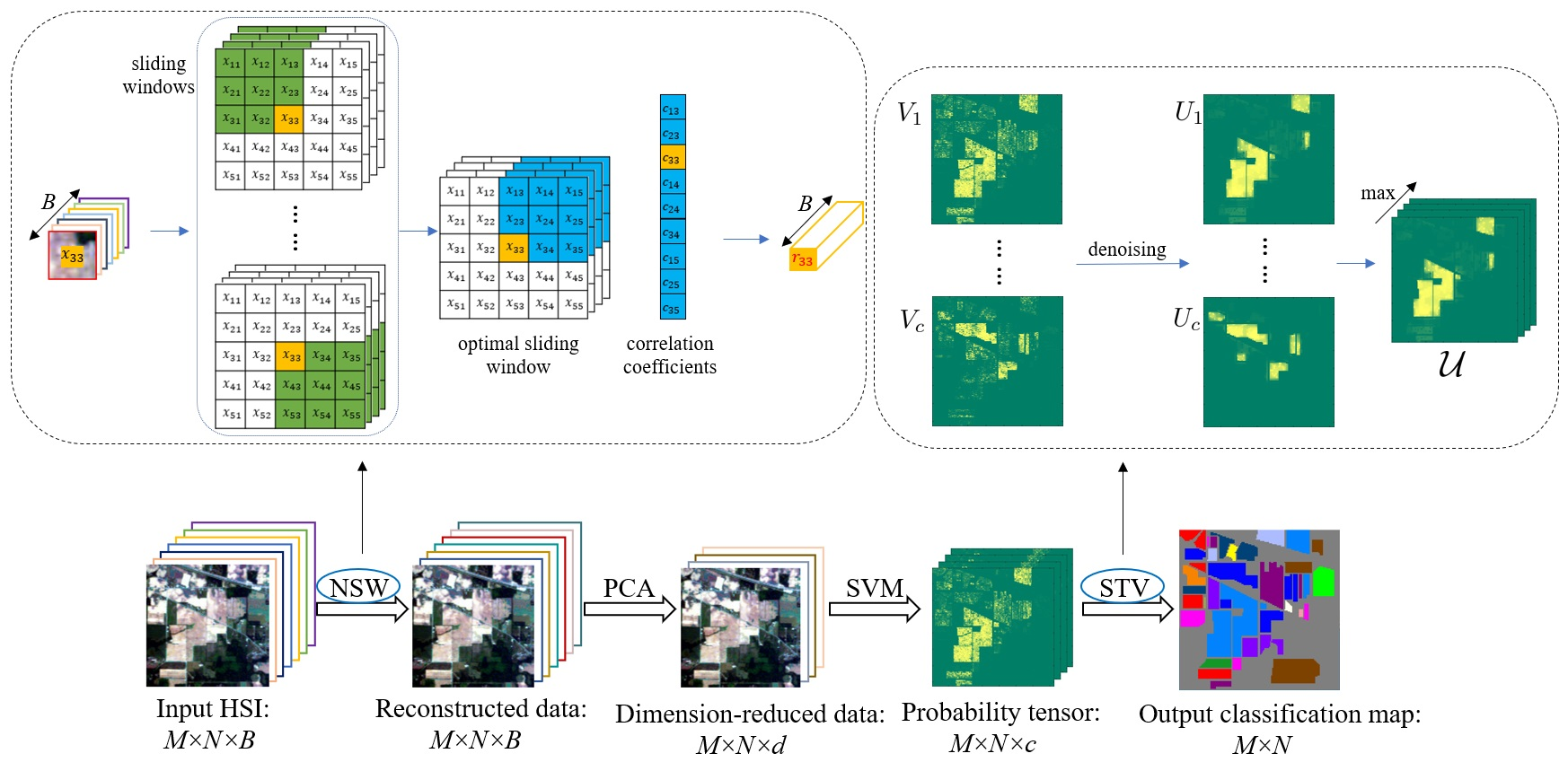
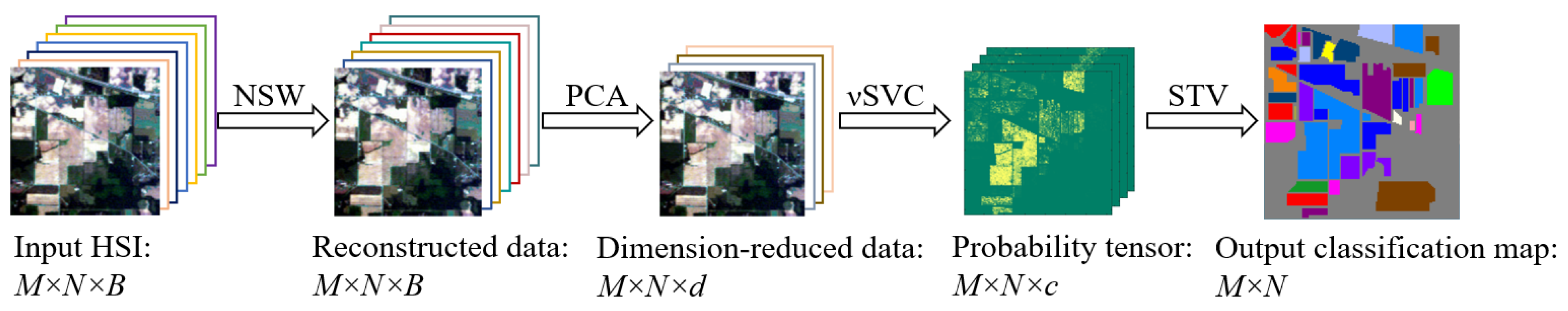
2. The Proposed Method
2.1. The Pre-Processing Stage
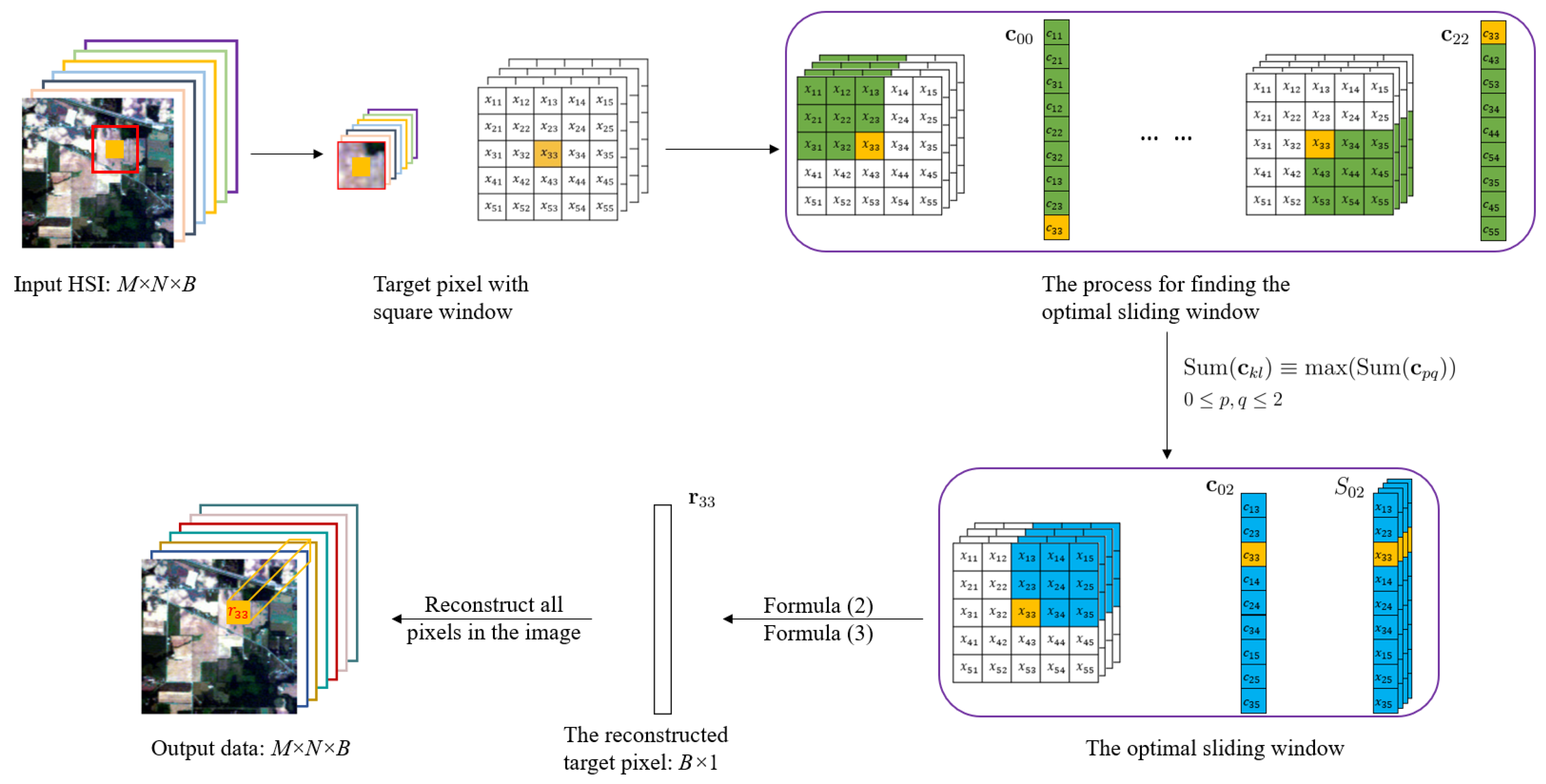
2.1.1. The Nested Sliding Window (NSW) Method
2.1.2. Principal Component Analysis (PCA)
2.2. The Pixel-Wise Classification Stage
2.3. The Smoothing Stage
3. Experimental Results
3.1. DataSets
3.2. Comparison Methods and Evaluation Metrics
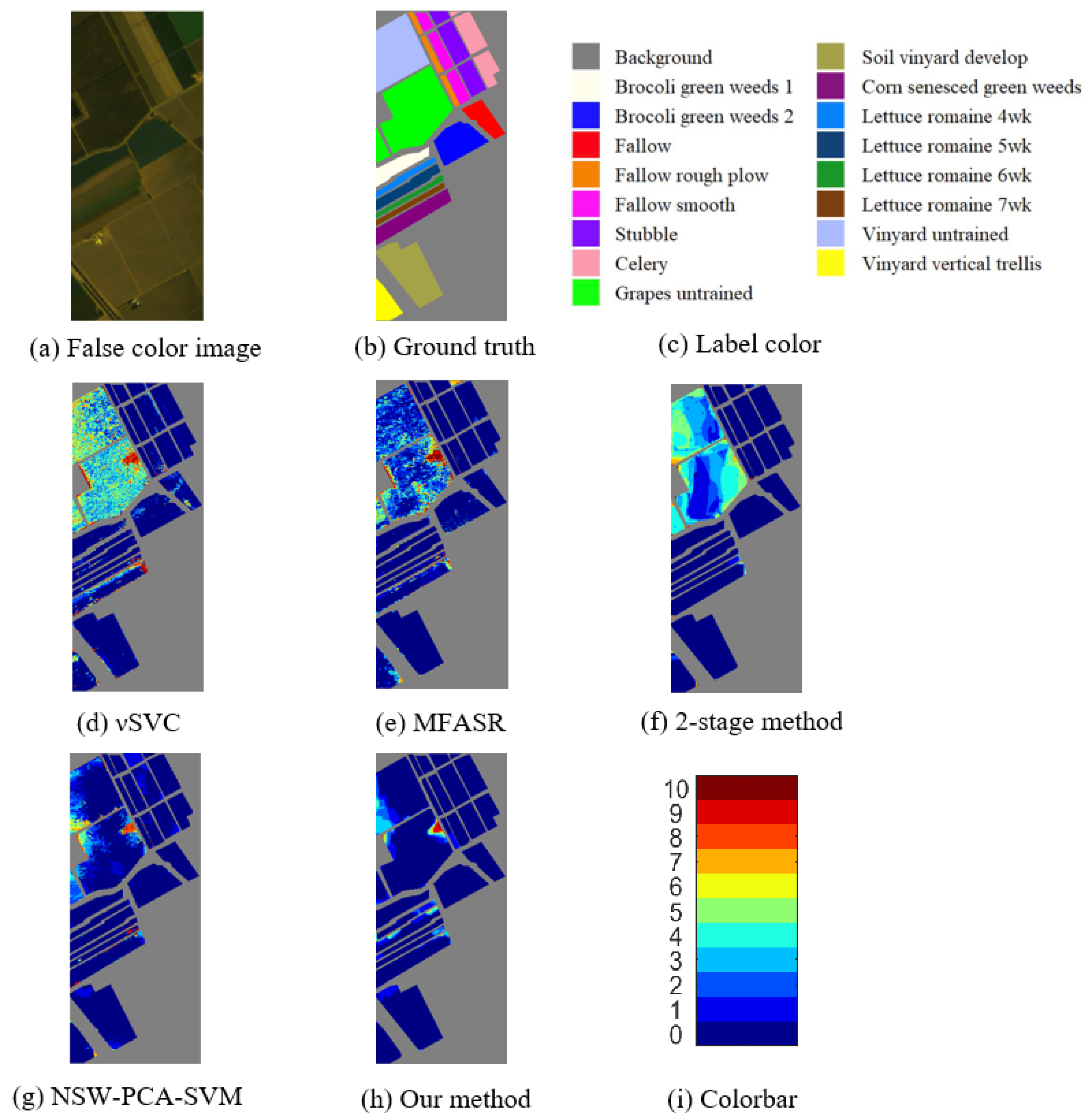
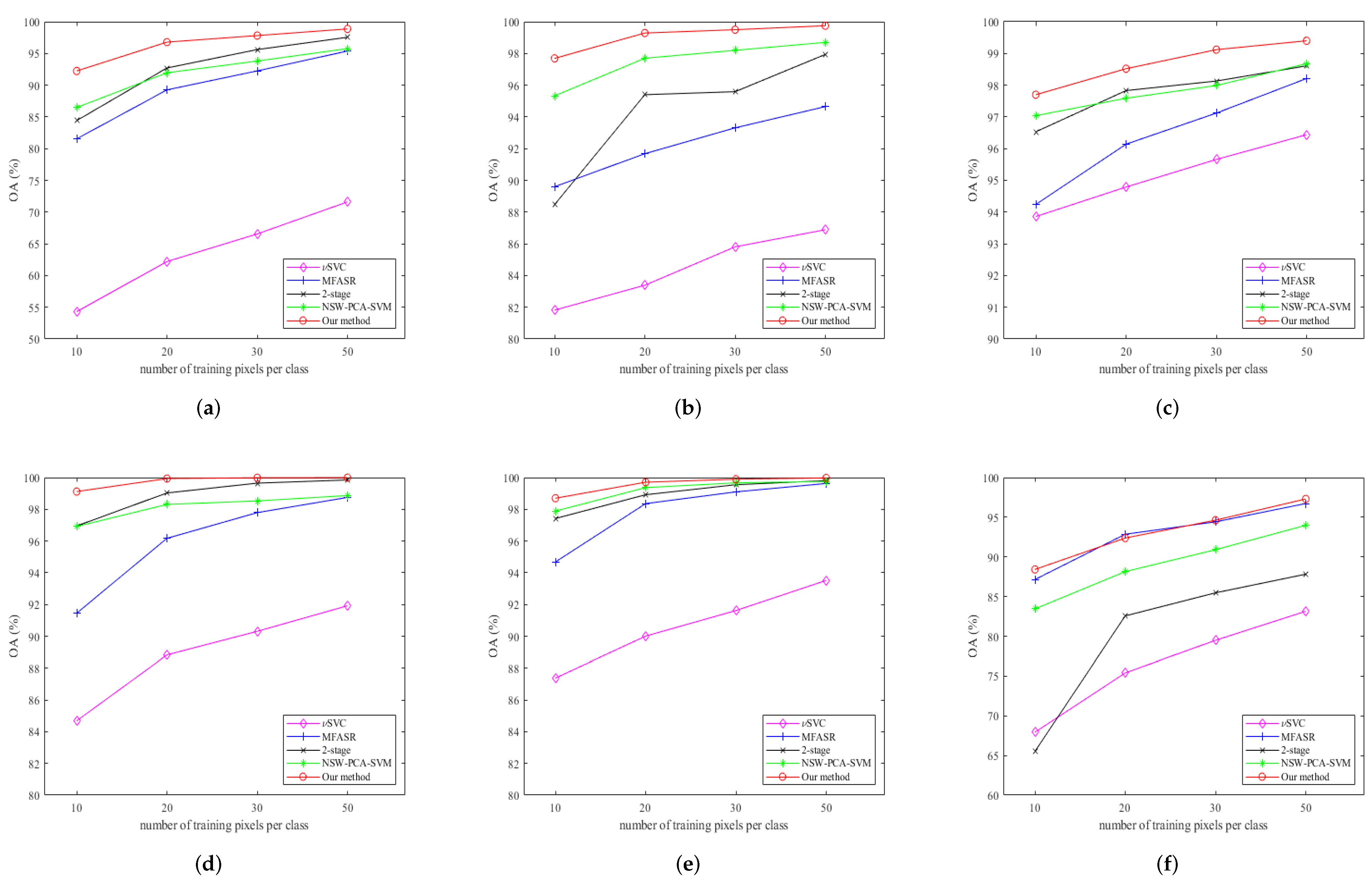
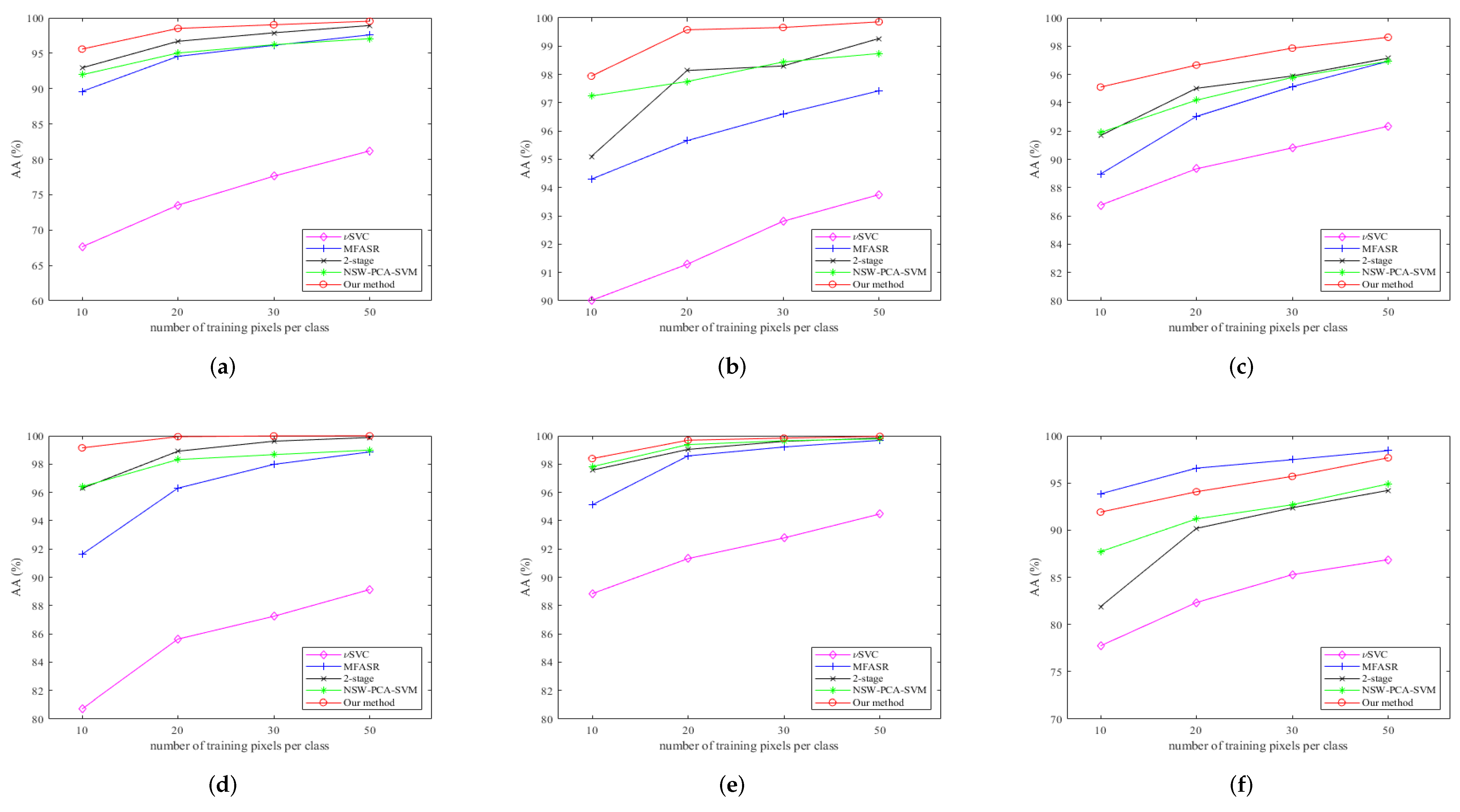
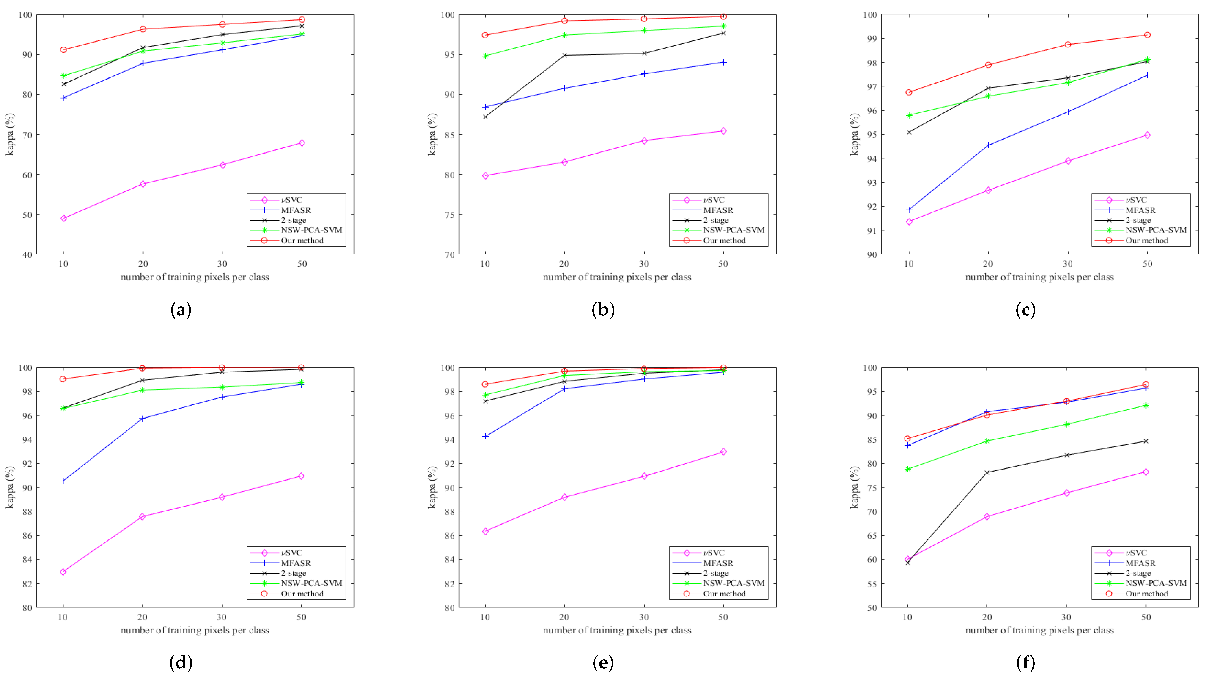
3.3. Classification Results
4. Discussion
4.1. Parameters for Each Method
4.2. The Influence of the Two Parameters in the Pre-Processing Stage
4.3. The Quality of Post-Processing Step
4.4. Computation Times for Each Method
4.5. Summary of Each Method
5. Conclusions
Author Contributions
Funding
Data Availability Statement
Acknowledgments
Conflicts of Interest
References
- Eismann, M.T. Hyperspectral Remote Sensing, 1st ed.; SPIE Press: Bellingham, WA, USA, 2012; pp. 1–33. [Google Scholar]
- Morchhale, S.; Pauca, V.P.; Plemmons, R.J.; Torgersen, T.C. Classification of Pixel-Level Fused Hyperspectral and Lidar Data Using Deep Convolutional Neural Networks. In Proceedings of the 2016 8th Workshop on Hyperspectral Image and Signal Processing: Evolution in Remote Sensing (WHISPERS), Los Angeles, CA, USA, 21–24 August 2016; pp. 1–5. [Google Scholar]
- Liu, S.; Marinelli, D.; Bruzzone, L.; Bovolo, F. A Review of Change Detection in Multitemporal Hyperspectral Images: Current Techniques, Applications, and Challenges. IEEE Geosci. Remote Sens. Mag. 2019, 7, 140–158. [Google Scholar] [CrossRef]
- Khan, M.J.; Khan, H.S.; Yousaf, A.; Khurshid, K.; Abbas, A. Modern Trends in Hyperspectral Image Analysis: A Review. IEEE Access 2018, 6, 14118–14129. [Google Scholar] [CrossRef]
- Peyghambari, S.; Zhang, Y. Hyperspectral Remote Sensing in Lithological Mapping, Mineral Exploration, and Environmental Geology: An Updated Review. J. Appl. Remote Sens. 2021, 15, 1–25. [Google Scholar] [CrossRef]
- Polk, S.L.; Cui, K.; Plemmons, R.J.; Murphy, J.M. Diffusion and Volume Maximization-Based Clustering of Highly Mixed Hyperspectral Images. arXiv 2022, arXiv:2203.09992. [Google Scholar]
- Polk, S.L.; Cui, K.; Plemmons, R.J.; Murphy, J.M. Active Diffusion and VCA-Assisted Image Segmentation of Hyperspectral Images. arXiv 2022, arXiv:2204.06298. [Google Scholar]
- Camalan, S.; Cui, K.; Pauca, V.P.; Alqahtani, S.; Silman, M.; Chan, R.H.; Plemmons, R.J.; Dethier, E.N.; Fernandez, L.E.; Lutz, D. Change Detection of Amazonian Alluvial Gold Mining Using Deep Learning and Sentinel-2 Imagery. Remote Sens. 2022, 14, 1746. [Google Scholar] [CrossRef]
- Cui, K.; Plemmons, R.J. Unsupervised Classification of AVIRIS-NG Hyperspectral Images. In Proceedings of the 2021 11th Workshop on Hyperspectral Imaging and Signal Processing: Evolution in Remote Sensing (WHISPERS), Amsterdam, The Netherlands, 24–26 March 2021; pp. 1–5. [Google Scholar]
- Im, J.; Jensen, J.R.; Jensen, R.R.; Gladden, J.; Waugh, J.; Serrato, M. Vegetation Cover Analysis of Hazardous Waste Sites in Utah and Arizona Using Hyperspectral Remote Sensing. Remote Sens. 2012, 4, 327–353. [Google Scholar] [CrossRef]
- Hörig, B.; Kühn, F.; Oschütz, F.; Lehmann, F. HyMap Hyperspectral Remote Sensing to Detect Hydrocarbons. Int. J. Remote Sens. 2001, 22, 1413–1422. [Google Scholar] [CrossRef]
- Qin, Q.; Zhang, Z.; Chen, L.; Wang, N.; Zhang, C. Oil and Gas Reservoir Exploration Based on Hyperspectral Remote Sensing and Super-Low-Frequency Electromagnetic Detection. J. Appl. Remote Sens. 2016, 10, 1–18. [Google Scholar] [CrossRef]
- Jin, X.; Jie, L.; Wang, S.; Qi, H.J.; Li, S.W. Classifying Wheat Hyperspectral Pixels of Healthy Heads and Fusarium Head Blight Disease Using a Deep Neural Network in the Wild Field. Remote Sens. 2018, 10, 395. [Google Scholar] [CrossRef]
- Neupane, K.; Baysal-Gurel, F. Automatic Identification and Monitoring of Plant Diseases Using Unmanned Aerial Vehicles: A Review. Remote Sens. 2021, 13, 3841. [Google Scholar] [CrossRef]
- Chan, A.H.Y.; Barnes, C.; Swinfield, T.; Coomes, D.A. Monitoring Ash Dieback (Hymenoscyphus Fraxineus) in British Forests Using Hyperspectral Remote Sensing. Remote Sens. Ecol. Conserv. 2021, 7, 306–320. [Google Scholar] [CrossRef]
- Polk, S.L.; Chan, A.H.Y.; Cui, K.; Plemmons, R.J.; Coomes, D.; Murphy, J.M. Unsupervised Detection of Ash Dieback Disease (Hymenoscyphus Fraxineus) Using Diffusion-Based Hyperspectral Image Clustering. arXiv 2022, arXiv:2204.09041. [Google Scholar]
- Lv, W.; Wang, X. Overview of Hyperspectral Image Classification. J. Sens. 2020, 2020, 4817234. [Google Scholar] [CrossRef]
- Melgani, F.; Bruzzone, L. Classification of Hyperspectral Remote Sensing Images with Support Vector Machines. IEEE Trans. Geosci. Remote Sens. 2004, 42, 1778–1790. [Google Scholar] [CrossRef]
- Kuo, B.; Yang, J.; Sheu, T.; Yang, S. Kernel-Based KNN and Gaussian Classifiers for Hyperspectral Image Classification. In Proceedings of the IGARSS 2008—2008 IEEE International Geoscience and Remote Sensing Symposium, Boston, MA, USA, 7–11 July 2008; pp. II-1006–II-1008. [Google Scholar]
- Li, J.; Bioucas-Dias, J.M.; Plaza, A. Semisupervised Hyperspectral Image Classification Using Soft Sparse Multinomial Logistic Regression. IEEE Geosci. Remote Sens. Lett. 2013, 10, 318–322. [Google Scholar]
- Ham, J.; Chen, Y.; Crawford, M.M.; Ghosh, J. Investigation of the Random Forest Framework for Classification of Hyperspectral Data. IEEE Trans. Geosci. Remote Sens. 2005, 43, 492–501. [Google Scholar] [CrossRef]
- Breiman, L. Random Forests. Mach. Learn. 2001, 45, 5–32. [Google Scholar] [CrossRef]
- Bo, C.; Lu, H.; Wang, D. Weighted Generalized Nearest Neighbor for Hyperspectral Image Classification. IEEE Access 2017, 5, 1496–1509. [Google Scholar] [CrossRef]
- Liu, J.; Wu, Z.; Wei, Z.; Xiao, L.; Sun, L. Spatial-Spectral Kernel Sparse Representation for Hyperspectral Image Classification. IEEE J. Sel. Top. Appl. Earth Observ. Remote Sens. 2013, 6, 2462–2471. [Google Scholar] [CrossRef]
- Cao, F.; Yang, Z.; Ren, J.; Ling, W.-K.; Zhao, H.; Marshall, S. Extreme Sparse Multinomial Logistic Regression: A Fast and Robust Framework for Hyperspectral Image Classification. Remote Sens. 2017, 9, 1255. [Google Scholar] [CrossRef]
- Gao, F.; Wang, Q.; Dong, J.; Xu, Q. Spectral and Spatial Classification of Hyperspectral Images Based on Random Multi-Graphs. Remote Sens. 2018, 10, 1271. [Google Scholar] [CrossRef]
- Zhang, Q.; Sun, J.; Zhong, G.; Dong, J. Random Multi-Graphs: A Semi-supervised Learning Framework for Classification of High Dimensional Data. Image Vis. Comput. 2017, 60, 30–37. [Google Scholar] [CrossRef]
- Shu, L.; McIsaac, K.; Osinski, G.R. Learning Spatial-Spectral Features for Hyperspectral Image Classification. IEEE Trans. Geosci. Remote Sens. 2018, 56, 5138–5147. [Google Scholar] [CrossRef]
- Camps-Valls, G.; Gomez-Chova, L.; Muñoz-Marí, J.; Vila-Francés, J.; Calpe-Maravilla, J. Composite Kernels for Hyperspectral Image Classification. IEEE Geosci. Remote Sens. Lett. 2006, 3, 93–97. [Google Scholar] [CrossRef]
- Rajadell, O.; Garcia-Sevilla, P.; Pla, F. Spectral-Spatial Pixel Characterization Using Gabor Filters for Hyperspectral Image Classification. IEEE Geosci. Remote Sens. Lett. 2013, 10, 860–864. [Google Scholar] [CrossRef]
- Bau, T.C.; Sarkar, S.; Healey, G. Hyperspectral Region Classification Using a Three-Dimensional Gabor Filterbank. IEEE Trans. Geosci. Remote Sens. 2010, 48, 3457–3464. [Google Scholar] [CrossRef]
- Fauvel, M.; Tarabalka, Y.; Benediktsson, J.A.; Chanussot, J.; Tilton, J.C. Advances in Spectral-Spatial Classification of Hyperspectral Images. Proc. IEEE 2013, 101, 652–675. [Google Scholar] [CrossRef]
- Fang, L.; Wang, C.; Li, S.; Benediktsson, J.A. Hyperspectral Image Classification via Multiple-Feature-Based Adaptive Sparse Representation. IEEE Trans. Instrum. Meas. 2017, 66, 1646–1657. [Google Scholar] [CrossRef]
- Gan, L.; Xia, J.; Du, P.; Chanussot, J. Multiple Feature Kernel Sparse Representation Classifier for Hyperspectral Imagery. IEEE Trans. Geosci. Remote Sens. 2018, 56, 5343–5356. [Google Scholar] [CrossRef]
- Chan, R.H.; Kan, K.K.; Nikolova, M.; Plemmons, R.J. A Two-Stage Method for Spectral–Spatial Classification of Hyperspectral Images. J. Math. Imaging Vis. 2020, 62, 790–807. [Google Scholar] [CrossRef]
- Ren, J.; Wang, R.; Liu, G.; Wang, Y.; Wu, W. An SVM-Based Nested Sliding Window Approach for Spectral-Spatial Classification of Hyperspectral Images. Remote Sens. 2021, 13, 114. [Google Scholar] [CrossRef]
- Yu, S.; Jia, S.; Xu, C. Convolutional Neural Networks for Hyperspectral Image Classification. Neurocomputing 2017, 219, 88–98. [Google Scholar] [CrossRef]
- Gao, Q.; Lim, S.; Jia, X. Hyperspectral Image Classification Using Convolutional Neural Networks and Multiple Feature Learning. Remote Sens. 2018, 10, 299. [Google Scholar] [CrossRef]
- Zhang, M.; Li, W.; Du, Q. Diverse Region-Based CNN for Hyperspectral Image Classification. IEEE Trans. Image Process. 2018, 27, 2623–2634. [Google Scholar] [CrossRef] [PubMed]
- Yang, X.; Ye, Y.; Li, X.; Lau, R.Y.K.; Zhang, X.; Huang, X. Hyperspectral Image Classification With Deep Learning Models. IEEE Trans. Geosci. Remote Sens. 2018, 56, 5408–5423. [Google Scholar] [CrossRef]
- Schölkopf, B.; Smola, A.J.; Williamson, R.C.; Bartlett, P.L. New Support Vector Algorithms. Neural Comput. 2000, 12, 1207–1245. [Google Scholar] [CrossRef]
- Luo, G.; Chen, G.; Tian, L.; Qin, K.; Qian, S. Minimum Noise Fraction versus Principal Component Analysis as a Preprocessing Step for Hyperspectral Imagery Denoising. Can. J. Remote Sens. 2016, 42, 106–116. [Google Scholar] [CrossRef]
- Hsu, C.-W.; Lin, C.-J. A Comparison of Methods for Multiclass Support Vector Machines. IEEE Trans. Neural Netw. 2002, 13, 415–425. [Google Scholar]
- Lin, H.-T.; Lin, C.-J.; Weng, R.C. A Note on Platt’s Probabilistic Outputs for Support Vector Machines. Mach. Learn. 2007, 68, 267–276. [Google Scholar] [CrossRef]
- Wu, T.-F.; Lin, C.-J.; Weng, R.C. Probability Estimates for Multi-Class Classification by Pairwise Coupling. J. Mach. Learn. Res. 2004, 5, 975–1005. [Google Scholar]
- Mumford, D.; Shah, J. Optimal Approximations by Piecewise Smooth Functions and Associated Variational Problems. Commun. Pure Appl. Math. 1989, 42, 577–685. [Google Scholar] [CrossRef]
- Fu, W.; Li, S.; Fang, L.; Kang, X.; Benediktsson, J.A. Hyperspectral Image Classification Via Shape-Adaptive Joint Sparse Representation. IEEE J. Sel. Top. Appl. Earth Observ. Remote Sens. 2016, 9, 556–567. [Google Scholar] [CrossRef]
- Katkovnik, V.; Egiazarian, K.; Astola, J. Local Approximation Techniques in Signal and Image Processing, 1st ed.; SPIE Press: Bellingham, WA, USA, 2006; pp. 139–193. [Google Scholar]
- Foi, A.; Katkovnik, V.; Egiazarian, K. Pointwise shape-adaptive DCT for high-quality denoising and deblocking of grayscale and color images. IEEE Trans. Image Process 2007, 16, 1395–1411. [Google Scholar] [CrossRef]
- Li, R.; Cui, K.; Chan, R.H.; Plemmons, R.J. Classification of Hyperspectral Images Using SVM with Shape-adaptive Reconstruction and Smoothed Total Variation. arXiv 2022, arXiv:2203.15619. [Google Scholar]
- Bazine, R.; Wu, H.; Boukhechba, K. Spatial Filtering in DCT Domain-Based Frameworks for Hyperspectral Imagery Classification. Remote Sens. 2019, 11, 1405. [Google Scholar] [CrossRef]
- Goodfellow, I.; Bengio, Y.; Courville, A. Deep Learning, 1st ed.; MIT Press: Cambridge, MA, USA, 2016; pp. 492–502. [Google Scholar]
- Pontil, M.; Verri, A. Support Vector Machines for 3d Object Recognition. IEEE Trans. Pattern Anal. Mach. Intell. 1998, 6, 637–646. [Google Scholar] [CrossRef]
- El-Naqa, I.; Yang, Y.; Wernick, M.N.; Galatsanos, N.P.; Nishikawa, R.M. A Support Vector Machine Approach for Detection of Microcalcifications. IEEE Trans. Med. Imaging 2002, 21, 1552–1563. [Google Scholar] [CrossRef]
- Osuna, E.; Freund, R.; Girosit, F.A. Training Support Vector Machines: An Application to Face Detection. In Proceedings of the IEEE Computer Society Conference on Computer Vision and Pattern Recognition, San Juan, PR, USA, 17–19 June 1997; pp. 130–136. [Google Scholar]
- Tay, F.E.H.; Cao, L. Application of Support Vector Machines in Financial Time Series Forecasting. Omega 2001, 29, 309–317. [Google Scholar] [CrossRef]
- Kim, K.-J. Financial Time Series Forecasting Using Support Vector Machines. Neurocomputing 2003, 55, 307–319. [Google Scholar] [CrossRef]
- Cortes, C.; Vapnik, V. Support-Vector Networks. Mach. Learn. 1995, 20, 273–297. [Google Scholar] [CrossRef]
- Tarabalka, Y.; Fauvel, M.; Chanussot, J.; Benediktsson, J.A. SVM- and MRF-Based Method for Accurate Classification of Hyperspectral Images. IEEE Geosci. Remote Sens. Lett. 2010, 7, 736–740. [Google Scholar] [CrossRef]
- Chakravarty, S.; Banerjee, M.; Chandel, S. Spectral-Spatial Classification of Hyperspectral Imagery Using Support Vector and Fuzzy-MRF. In Proceedings of the International Conference on Intelligent, Secure, and Dependable Systems in Distributed and Cloud Environments, Vancouver, BC, Canada, 25–27 October 2017; pp. 151–161. [Google Scholar]
- Boyd, S.; Parikh, N.; Chu, E.; Peleato, B.; Eckstein, J. Distributed Optimization and Statistical Learning via the Alternating Direction Method of Multipliers. Found. Trends Mach. Learn. 2011, 3, 1–122. [Google Scholar] [CrossRef]
- Cohen, J. A Coefficient of Agreement for Nominal Scales. Educ. Psychol. Meas. 1960, 20, 37–46. [Google Scholar] [CrossRef]
- Story, M.; Congalton, R.G. Accuracy Assessment: A User’s Perspective. Photogramm. Eng. Remote Sens. 1986, 52, 397–399. [Google Scholar]
- Kohavi, R. A Study of Cross-Validation and Bootstrap for Accuracy Estimation and Model Selection. In Proceedings of the 14th International Joint Conference on Artificial Intelligence, Montreal, QC, Canada, 20–25 August 1995; pp. 1137–1143. [Google Scholar]


| Class | SVC | MFASR | 2-Stage Method | NSW-PCA-SVM | Our Method |
|---|---|---|---|---|---|
| Alfalfa | 82.22% | 97.50% | 98.89% | 97.50% | 100% |
| Corn-no till | 39.32% | 70.87% | 75.05% | 77.35% | 82.53% |
| Corn-mill till | 49.05% | 79.38% | 91.26% | 89.68% | 92.06% |
| Corn | 63.83% | 87.49% | 100% | 89.74% | 98.19% |
| Grass/pasture | 77.61% | 84.84% | 88.37% | 86.17% | 90.87% |
| Grass/trees | 80.97% | 92.35% | 99.04% | 97.44% | 99.51% |
| Grass/pasture-mowed | 93.33% | 100% | 100% | 100% | 100% |
| Hay-windrowed | 72.12% | 99.38% | 100% | 99.83% | 100% |
| Oats | 96.00% | 100% | 100% | 100% | 100% |
| Soybeans-no till | 52.92% | 81.70% | 85.21% | 87.43% | 90.88% |
| Soybeans-mill till | 42.76% | 69.79% | 66.72% | 78.00% | 91.04% |
| Soybeans-clean | 36.59% | 83.05% | 90.81% | 80.57% | 91.75% |
| Wheat | 92.36% | 99.49% | 99.59% | 98.67% | 100% |
| Woods | 67.55% | 92.77% | 94.96% | 95.24% | 95.88% |
| Bridg-Grass-Tree-Drives | 41.81% | 95.35% | 97.23% | 96.54% | 96.73% |
| Stone-steel lowers | 93.61% | 99.16% | 99.88% | 97.23% | 100% |
| OA | 54.31% | 81.54% | 84.42% | 86.48% | 92.24% |
| AA | 67.63% | 89.60% | 92.94% | 91.96% | 95.59% |
| kappa | 49.00% | 79.15% | 82.54% | 84.68% | 91.16% |
| Class | SVC | MFASR | 2-Stage Method | NSW-PCA-SVM | Our Method |
|---|---|---|---|---|---|
| Broccoli-green-weeds-1 | 98.02% | 99.14% | 99.84% | 99.86% | 100% |
| Broccoli-green-weeds-2 | 97.70% | 97.75% | 99.78% | 99.82% | 100% |
| Fallow | 92.84% | 99.06% | 99.35% | 99.92% | 99.99% |
| Fallow-rough-plow | 98.64% | 99.65% | 98.17% | 99.92% | 97.83% |
| Fallow-smooth | 95.57% | 98.89% | 99.00% | 98.80% | 99.64% |
| Stubble | 97.90% | 99.70% | 99.32% | 96.89% | 99.94% |
| Celery | 98.74% | 97.02% | 99.12% | 99.71% | 99.96% |
| Grapes-untrained | 55.77% | 70.16% | 70.26% | 88.95% | 96.12% |
| Soil-vineyard-develop | 97.35% | 99.47% | 99.78% | 98.80% | 99.21% |
| Corn-senesced-green-weeds | 79.17% | 89.54% | 98.54% | 95.77% | 98.44% |
| Lettuce-romaine-4wk | 92.02% | 97.58% | 99.36% | 99.40% | 94.24% |
| Lettuce-romaine-5wk | 97.52% | 99.54% | 99.73% | 99.79% | 92.61% |
| Lettuce-romaine-6wk | 98.18% | 97.74% | 99.64% | 97.70% | 99.01% |
| Lettuce-romaine-7wk | 89.58% | 92.87% | 97.78% | 92.59% | 96.06% |
| Vinyard-untrained | 57.49% | 82.98% | 64.19% | 89.79% | 94.42% |
| Vinyard-vertical-trellis | 93.71% | 92.06% | 97.79% | 98.12% | 99.54% |
| OA | 81.82% | 89.78% | 88.47% | 95.33% | 97.69% |
| AA | 90.01% | 94.57% | 95.10% | 97.24% | 97.94% |
| kappa | 79.85% | 88.66% | 87.18% | 94.81% | 97.43% |
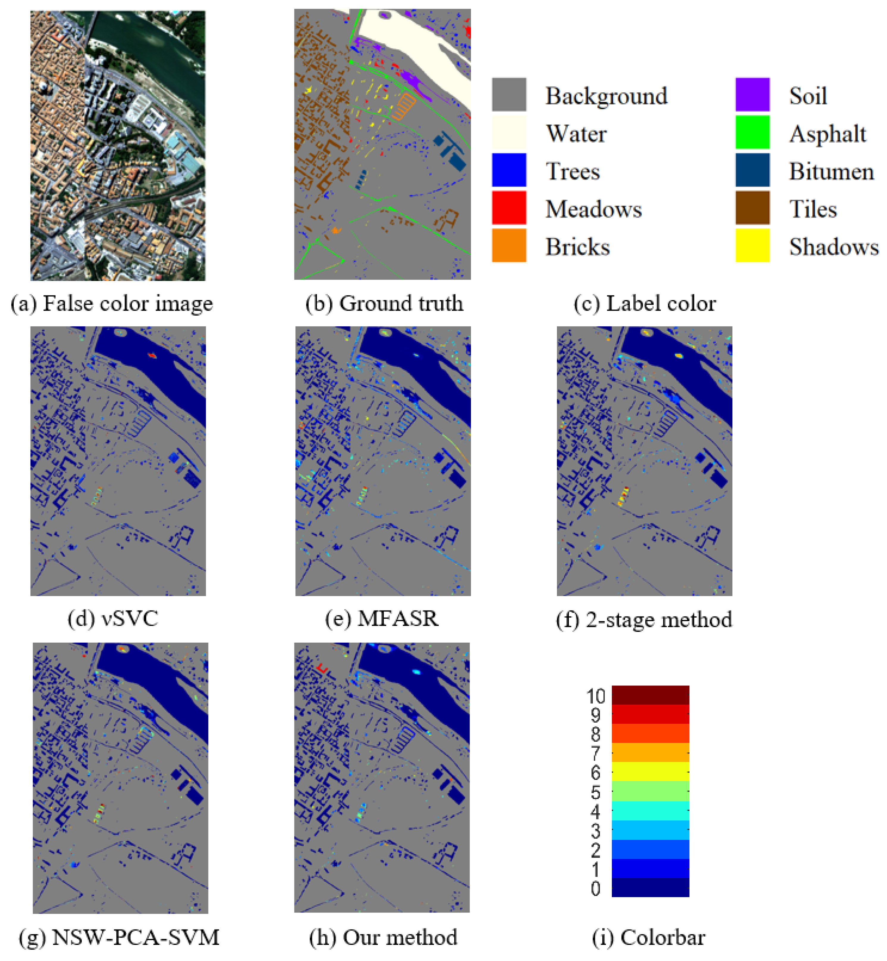
| Class | SVC | MFASR | 2-Stage Method | NSW-PCA-SVM | Our Method |
|---|---|---|---|---|---|
| Water | 99.02% | 99.78% | 99.56% | 100% | 99.48% |
| Trees | 81.58% | 75.56% | 76.29% | 85.99% | 91.15% |
| Meadows | 80.78% | 78.63% | 88.21% | 89.64% | 90.41% |
| Bricks | 75.65% | 92.40% | 92.70% | 81.42% | 96.03% |
| Soil | 78.80% | 88.57% | 84.58% | 89.90% | 91.97% |
| Asphalt | 89.26% | 85.62% | 97.70% | 93.40% | 97.96% |
| Bitumen | 80.64% | 89.92% | 87.64% | 88.30% | 94.08% |
| Tiles | 95.33% | 94.01% | 99.18% | 99.15% | 98.26% |
| Shadows | 99.74% | 97.13% | 99.30% | 99.27% | 96.62% |
| OA | 93.86% | 94.38% | 96.53% | 97.04% | 97.70% |
| AA | 86.76% | 89.07% | 91.68% | 91.90% | 95.11% |
| kappa | 91.37% | 92.09% | 95.09% | 95.80% | 96.75% |
| SVC | MFASR | 2-Stage Method | NSW-PCA-SVM | Our Method | |
|---|---|---|---|---|---|
| Number of parameters | 2 | 10 | 5 | 4 | 7 |
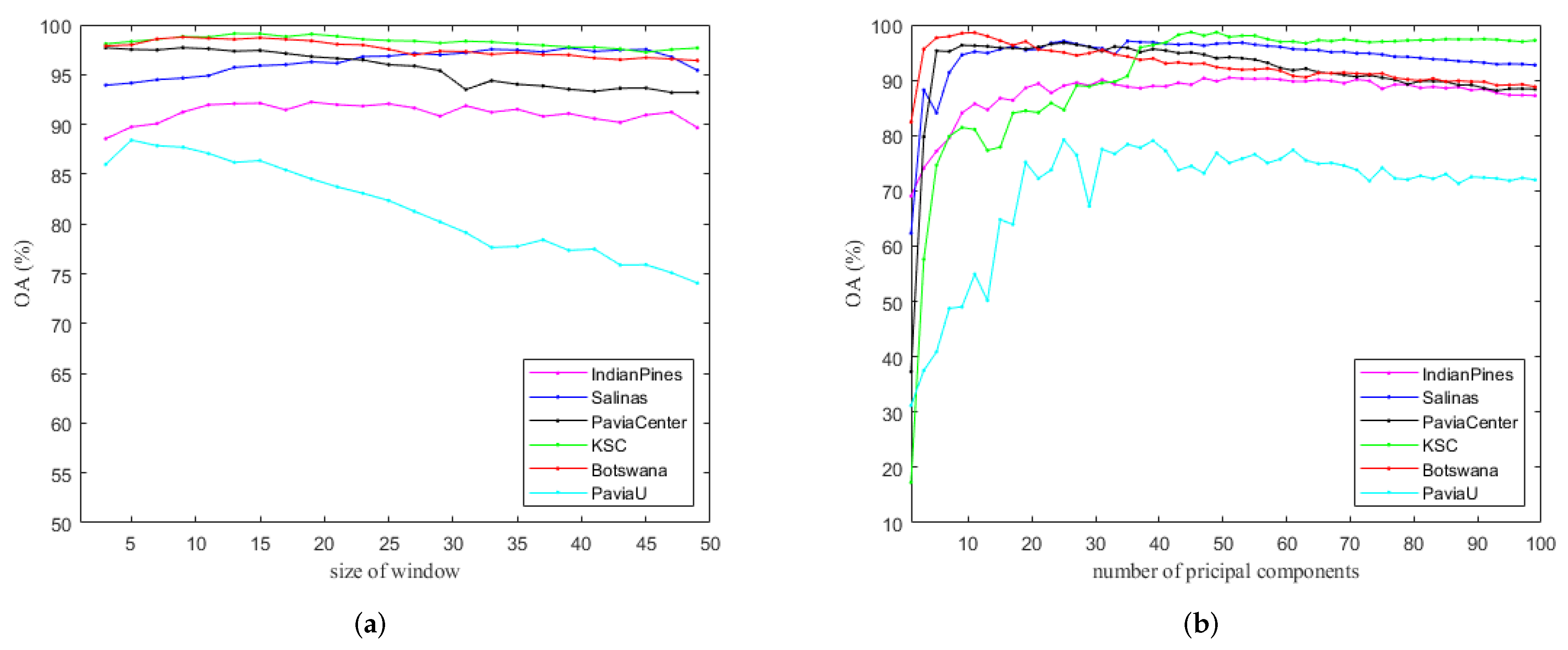
| Size of Window () | Principal Component Number (d) | |
|---|---|---|
| Indian Pines | 19 | 52 |
| Salinas | 39 | 24 |
| Pavia Center | 9 | 25 |
| KSC | 9 | 45 |
| Botswana | 15 | 11 |
| PaviaU | 5 | 39 |
| Gain | |||
|---|---|---|---|
| Indian Pines | 22.68 | 33.37 | 12.32 |
| Salinas | 21.05 | 27.16 | 6.11 |
| Pavia Center | 24.78 | 28.90 | 4.12 |
| KSC | 35.10 | 47.38 | 12.28 |
| Botswana | 38.21 | 54.65 | 16.44 |
| PaviaU | 23.12 | 28.35 | 5.23 |
| SVC | MFASR | 2-Stage Method | NSW-PCA-SVM | Our Method | |
|---|---|---|---|---|---|
| Indian Pines | 4.330 | 279.069 | 9.220 | 2767.587 | 1943.242 |
| Salinas | 16.595 | 1477.910 | 95.119 | 49,277.255 | 153,536.181 |
| Pavia Center | 36.954 | 3183.543 | 255.212 | 4081.842 | 4168.063 |
| KSC | 2.152 | 69.498 | 57.687 | 640.146 | 157.427 |
| Botswana | 1.708 | 81.848 | 65.990 | 583.016 | 329.433 |
| PaviaU | 5.045 | 893.491 | 58.547 | 271.707 | 350.894 |
| Methods | Features | Advantages | Limitations |
|---|---|---|---|
| SVC | spectral | shortest running time | lowest accuracy |
| MFASR | spectral, spatial | better performance for PaviaU dataset | lower accuracy, longer running time |
| 2-stage | spectral, spatial | shorter running time | misclassification of classes with similar spectra |
| NSW-PCA-SVM | spectral, spatial | higher accuracy with limited labeled pixels | longer running time |
| Our method | spectral, spatial | highest accuracy with limited labeled pixels, robust to parameters | longer running time |
Publisher’s Note: MDPI stays neutral with regard to jurisdictional claims in published maps and institutional affiliations. |
© 2022 by the authors. Licensee MDPI, Basel, Switzerland. This article is an open access article distributed under the terms and conditions of the Creative Commons Attribution (CC BY) license (https://creativecommons.org/licenses/by/4.0/).
Share and Cite
Chan, R.H.; Li, R. A 3-Stage Spectral-Spatial Method for Hyperspectral Image Classification. Remote Sens. 2022, 14, 3998. https://doi.org/10.3390/rs14163998
Chan RH, Li R. A 3-Stage Spectral-Spatial Method for Hyperspectral Image Classification. Remote Sensing. 2022; 14(16):3998. https://doi.org/10.3390/rs14163998
Chicago/Turabian StyleChan, Raymond H., and Ruoning Li. 2022. "A 3-Stage Spectral-Spatial Method for Hyperspectral Image Classification" Remote Sensing 14, no. 16: 3998. https://doi.org/10.3390/rs14163998