Article

Fusion of Multidimensional CNN and Handcrafted Features for Small-Sample Hyperspectral Image Classification

1
ATR Key Laboratory, Shenzhen University, Shenzhen 518060, China
2
Guangdong Key Laboratory of Intelligent Information Processing, Shenzhen University, Shenzhen 518060, China
*
Author to whom correspondence should be addressed.
Remote Sens. 2022, 14(15), 3796; https://doi.org/10.3390/rs14153796
Submission received: 30 June 2022 / Revised: 30 July 2022 / Accepted: 4 August 2022 / Published: 6 August 2022

Abstract

:
Hyperspectral image (HSI) classification has attracted widespread concern in recent years. However, due to the complexity of the HSI gathering environment, it is difficult to obtain a great number of HSI labeled samples. Therefore, how to effectively extract the spatial–spectral feature with small-scale training samples is the crucial point of HSI classification. In this paper, a novel fusion framework for small-sample HSI classification is proposed to fully combine the advantages of multidimensional CNN and handcrafted features. Firstly, a 3D fuzzy histogram of oriented gradients (3D-FHOG) descriptor is proposed to fully extract the handcrafted spatial–spectral feature of HSI pixels, which is suggested to be more robust by overcoming the local spatial–spectral feature uncertainty. Secondly, a multidimensional Siamese network (MDSN), which is updated by minimizing both contrastive loss and classification loss, is designed to effectively exploit the CNN-based spatial–spectral features from multiple dimensions. Finally, the proposed MDSN combined with 3D-FHOG is utilized for small-sample HSI classification to verify the effectiveness of our proposed fusion framework. The experimental results on three public data sets indicate that the proposed MDSN combined with 3D-FHOG is significantly better than the representative handcrafted feature-based and CNN-based methods, which in turn demonstrates the superiority of the proposed fusion framework.

1. Introduction

Compared with gray-scale and RGB images, hyperspectral image (HSI) can provide a rich amount of spatial and spectral information of objects. Since the additional spectral information may help to overcome the existing difficulties of traditional image processing technology, HSI has attracted widespread concern in recent years. HSI classification [1,2,3,4], which is the focus of research in the field of HSI processing, has been widely applied in various areas, such as scene understanding [5,6], disease examination [7,8], face recognition [9,10] and city planning [11,12]. Note that the feature extracted from HSI is the basis of these applications, thus it is essential to obtain the more robust and effective spatial–spectral feature for HSI classification. However, due to the complexity and potential fatalness of the HSI acquisition environment, it is a laborious and time-consuming job to collect a huge amount of labeled samples. Therefore, how to effectively extract the spatial–spectral feature with small-scale training samples has become a hot spot of current research. Existing HSI feature extraction methods can be divided into two types: handcrafted feature extraction methods and deep feature extraction methods.
Before the development of deep learning, handcrafted feature extraction was the mainstream approach in the field of image processing, and its effectiveness has been verified in image matching and classification [13,14]. Lowe [13] designed an image feature extraction method called the scale-invariant feature transform (SIFT), which shows its robustness in object recognition. Local binary pattern (LBP) proposed by Ojala et al. [14] is a simple and efficient local feature descriptor, which is able to achieve gray-scale and rotation invariant texture classification. Meanwhile, since HSI can be represented as the 3D-structure data, many 3D handcrafted feature descriptors have been presented for the HSI feature extraction. Zhao et al. [15] designed the 3D-LBP operator to extract the dynamic feature from the spatial–temporal domain, which is an extension of LBP. Inspired by [15], Jia et al. [16] applied the 3D-LBP to the spatial–spectral domain of HSI, which exhibits excellent performance in HSI classification. He et al. [17] presented a 3D Gabor filter-based descriptor, which can be utilized to perform HSI classification in a computationally efficient way. The 3D discrete wavelet transform (3D-DWT) proposed by Cao et al. [18] can fully utilize the spatial–spectral information and improve the performance of HSI classification. However, due to the simple structure and fixed calculation pattern, handcrafted features are not robust when confronted with complex circumstances of HSI classification.
In recent years, with the development of hardware devices and the arrival of the big data era, deep learning technique has made great progress. Especially, convolutional neural network (CNN) is the most commonly used deep learning technique in the area of computer vision. Because of its local connection and nonlinear characteristic, making it able to extract the more discriminative feature, CNN is quite effective for image processing, including HSI classification. Sharma et al. [19] combined the band selection with 2D CNN-based features to enhance the performance of HSI classification, which outperforms the handcrafted feature-based methods. Meanwhile, 1D CNN and 1D recurrent neural network (RNN) features [20,21,22] were utilized to process HSI pixels as sequential data, which takes full advantage of spectral correlation and band-to-band variability. To fully exploit the spatial and spectral information, 3D CNN-based methods are also employed for HSI classification. Lee et al. [23] designed a deeper CNN architecture that uses 3D fully convolutional layers (FCN) to learn the more effective spatial–spectral feature. The semi-supervised 3D CNN-based algorithm proposed by Liu et al. [24] can simultaneously minimize the sum of supervised and unsupervised cost functions during training, which aims to solve the problem of limited labeled samples. Luo et al. [25] presented a 3D CNN framework for HSI classification, which exhibits a good trade-off between the number of training samples and the complexity of the network. Roy et al. [26] proposed a hybrid spectral CNN (HybridSN) for HSI classification, which combines advantages of both 3D CNN and 2D CNN. Although CNN-based methods can achieve state-of-the-art performance with sufficient labeled samples, they cannot provide a strict mathematical explanation for its decision making. In addition, HSI classification accuracy of CNN-based methods will significantly decrease in the scenery of small-scale training samples.
As can be seen from the literature, the handcrafted feature-based methods can provide a stricter mathematical explanation for the HSI feature extraction process, which makes it more reliable to be utilized in some high-sensitive areas, such as biomedicine and military. However, compared with CNN-based methods, the performance of handcrafted feature-based methods is not robust in some complicated HSI classification tasks. On the other hand, utilizing only the CNN-based feature causes the difficulty in achieving high accuracy with limited labeled samples, and lacks the strict mathematical explanation for its decision making. Therefore, it is essential to develop a HSI classification algorithm that combines the advantages of both handcrafted and CNN-based feature.
Small-sample classification has become an important research topic in the area of remote sensing. To tackle the challenge of small-scale training samples, the idea of transfer learning has been introduced in remote sensing scene classification. Rostami et al. [27] proposed a deep transfer learning-based algorithm for few-shot synthetic aperture radar (SAR) image classification, which is effective on the problem of ship classification in the SAR domain. Alajaji et al. [28] combined the prototypical network with pre-trained CNN for image embedding, which obtains excellent classification results on two remote sensing scene data set. To further extract the generalized features from source domain, attention mechanism and multi-scale feature fusion strategy [29,30] are introduced in remote sensing few-shot scene classification. However, most of the transfer learning-based algorithms utilize only the CNN-based feature, ignoring the superiority of handcrafted feature. Moreover, since there may be a mismatch between the source and target domain distributions, the performances of transfer learning-based algorithms are unpredictable. As a special type of remote sensing image, HSI can provide additional spectral information for feature extraction. It can be known that the handcrafted feature is more reliable and easier to carry out without training. Therefore, our proposed algorithm mainly focuses on how to utilize the handcrafted feature to enhance the performance of CNN-based models in the scenery of small-sample supervised learning.
It can be known that fusing different types of spatial–spectral features may cause the increase in computational cost. However, in terms of some special small-sample HSI classification tasks, more accurate classification results need to be achieved without considering the computational cost. To the best of our knowledge, there still lacks an in-depth study concentrated on utilizing the handcrafted feature to enhance the performance of CNN-based models in small-sample HSI classification. Therefore, we propose a fusion framework of multidimensional CNN and handcrafted features for small-sample HSI classification. Specifically, a multidimensional Siamese network (MDSN) combined with the 3D fuzzy histogram of oriented gradients (3D-FHOG) features is introduced to verify the effectiveness of our proposed fusion framework.
The main contribution of this paper includes the following three aspects.
(1)
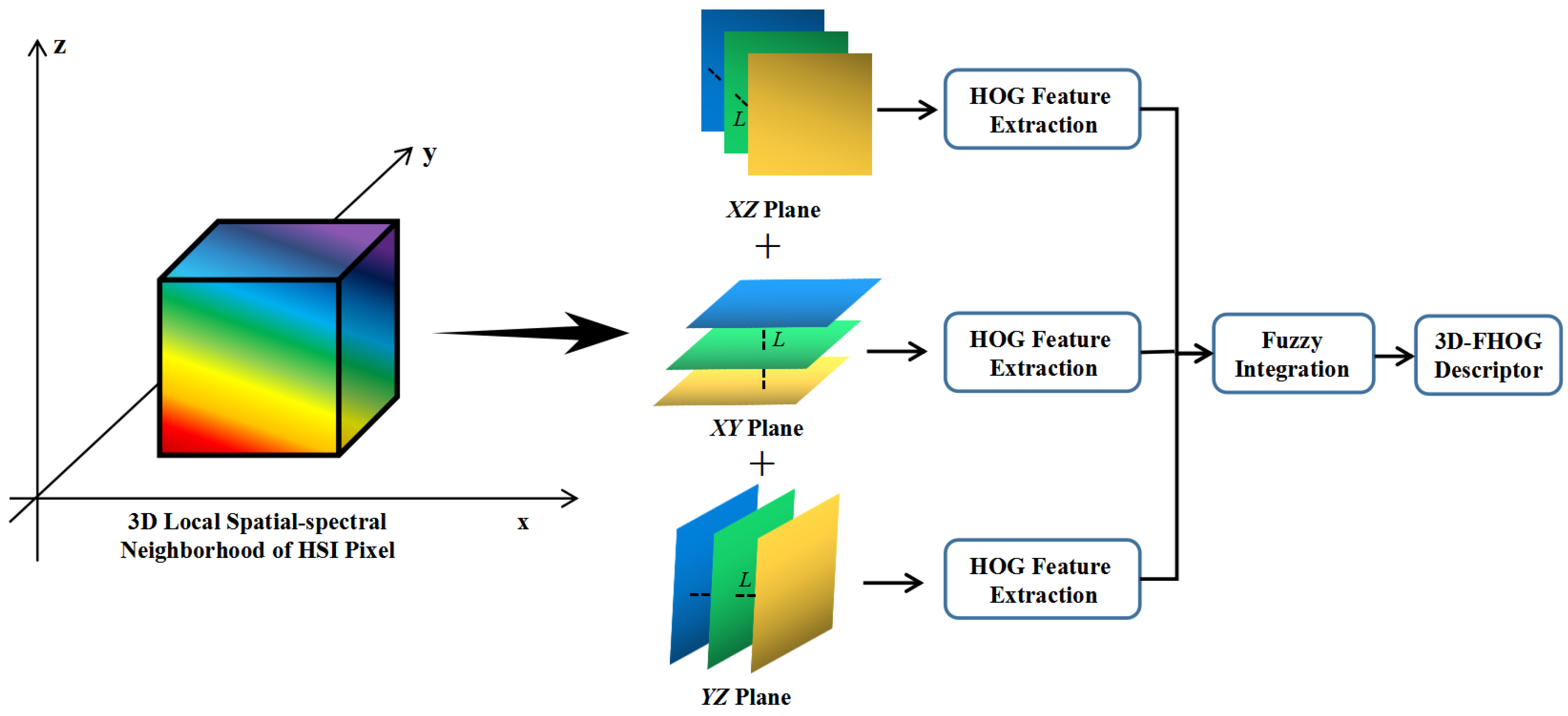
A 3D-FHOG descriptor is proposed to fully extract the handcrafted spatial–spectral feature of HSI pixels. It calculates the HOG features from three orthogonal planes to generate the final 3D-FHOG descriptor based on fuzzy fusion operation, which is able to overcome the local spatial–spectral feature uncertainty;
(2)
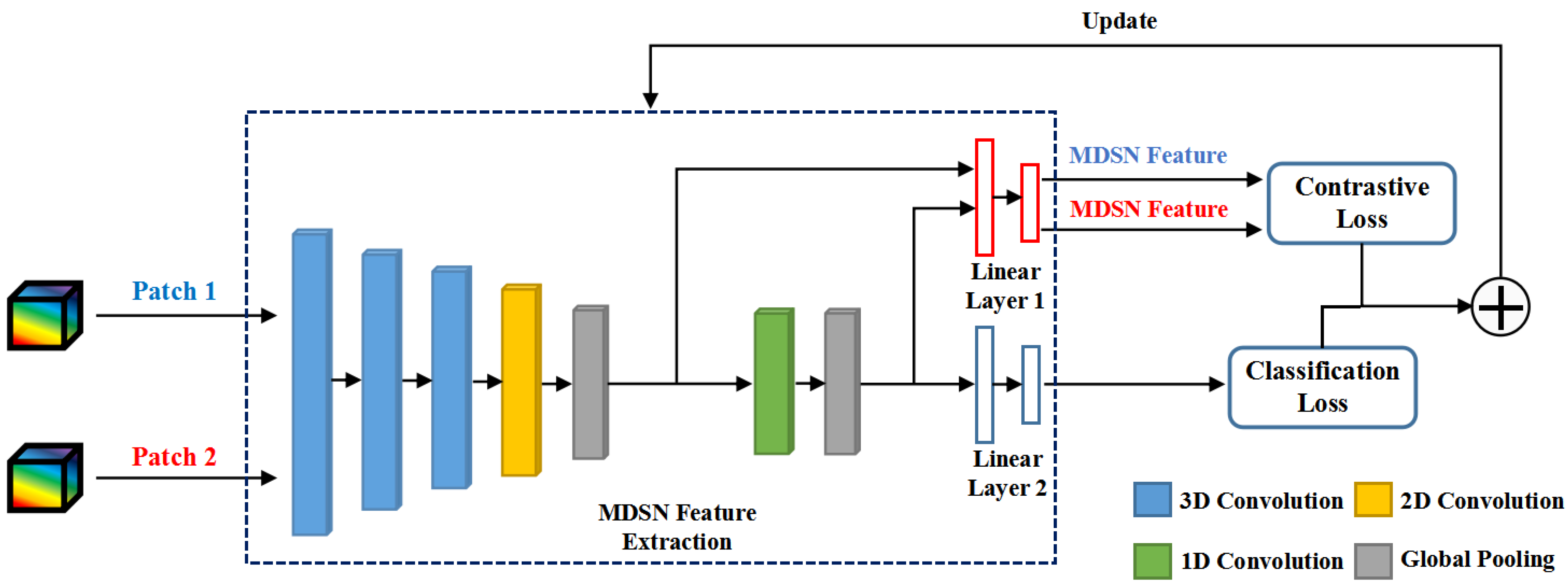
An effective Siamese network, i.e., MDSN is designed for further exploiting the multidimensional CNN-based spatial–spectral feature in the scenery of small-scale labeled samples. It mainly utilizes the hybrid 3D-2D-1D CNN to learn the spatial–spectral feature from multiple dimensions and is updated by minimizing both contrastive loss and classification loss. Compared with the single-dimensional CNN-based networks, the performance of MDSN is significantly better in small-sample HSI classification;
(3)
It provides a novel extensible fusion framework for the combination of hand- crafted and multidimensional CNN-based spatial–spectral features. More importantly, experimental results indicate that our proposed MDSN combined with 3D-FHOG features can achieve better performance than the handcrafted features-based and CNN-based algorithms, which in turn verifies the superiority of the proposed fusion framework.
The rest of this paper is organized as follows. Section 2 presents the related works of this study. The proposed methodology is presented in Section 3. Then, Section 4 reports the experimental results and discussions on three public data sets. Finally, a conclusion of this study is presented in Section 5.

2. Related Works

2.1. Histogram of Oriented Gradients

Histogram of oriented gradients (HOG) proposed by Dalal et al. [31] is a classical handcrafted feature descriptor, which is generated by computing the gradients of pixels in a local area. Additionally, it not only provides the rotation invariance and under- standability, but also has a strong capacity of shape feature expression, which makes it widely used in image recognition. Surasak et al. [32] applied the HOG algorithm to human detection in video, which is able to accurately obtain the number of people for each video frame. Mao et al. [33] utilized the HOG-based method and support vector machine (SVM) classifier to perform the preceding vehicle detection, which shows excellent performance in different traffic scenarios. Qi et al. [34] designed a ship histogram of oriented gradient (S-HOG) to characterize ship targets, which proved to be also effective when ship size varies. Since each HSI pixel corresponds to a spectral curve with different changing patterns, it is suggested that constructing the statistics histogram of local gradient change for HSI pixels is an effective solution for describing its local spatial–spectral features. Chen et al. [35] proposed a novel algorithm for hyperspectral face recognition by extracting the HOG feature, which outperforms several existing methods in the experiment. However, existing HOG-based algorithms ignore the characteristics of HSI, such as strong correlation between bands, vast amounts of redundant information and spatial–spectral feature uncertainty. Therefore, in this study, by introducing the fuzzy logic theory, we design a novel handcrafted feature descriptor named 3D-FHOG to fully exploit the spatial–spectral information and to overcome the spatial–spectral feature uncertainty.

2.2. Siamese Network
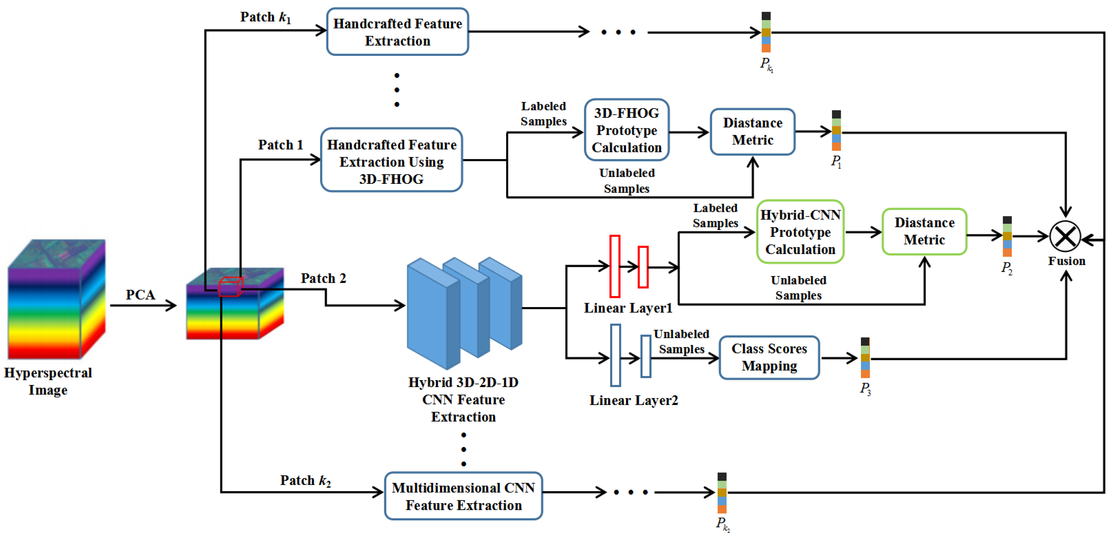
For the problem of small-scale labeled samples, it is suggested that a model named Siamese network [36,37] will be an effective solution for small-sample HSI classification. Specifically, Siamese network consists of two branches with the same architecture, and the image pairs are adopted as the input of Siamese network to minimize the contrastive loss. Early research of Siamese network mainly focuses on the application for target tracking. Tao et al. [38] first proposed to utilize the Siamese network in tracking tasks, which achieves state-of-the-art performance. Bertinetto et al. [39] designed a fully convolutional Siamese network to locate an exemplar image within a larger search image. Since the number of labeled samples will be augmented by generating the image pairs, Siamese network has been employed for few-shot classification tasks. Koch et al. [40] applied the Siamese network to the one-shot image recognition task, which obtains promising results. With respect to HSI classification, Zhao et al. [41] utilized the Siamese network to enlarge the training set and extract the effective spatial–spectral features, which is able to improve the classification performance. Liu et al. [42] proposed a Siamese network supervised with a margin ranking loss function for HSI classification, which can obtain better classification results than those of the conventional methods. Very recently, Cao et al. [43] designed a hybrid Siamese network called 3DCSN to perform HSI classification, which is suggested to be a robust and accurate classifier in the scenery of small-scale training samples. As described in [44], it can be known that the spatial–spectral features extracted from different CNN layers may contain the semantic information of objects with different scales. Therefore, in this paper, an effective Siamese network named MDSN is proposed to fully exploit the multidimensional CNN-based spatial–spectral feature. Moreover, we train the proposed MDSN by using both the contrastive loss function and classification loss function. Especially, our proposed MDSN is integrated with the idea of prototypical network in the testing phase, which is suggested to be more effective for small-sample HSI classification.

3. Methodology

The fusion framework of multidimensional CNN-based and handcrafted features for small-sample HSI classification is shown in Figure 1. In this study, to verify the effectiveness of our proposed fusion framework, we design the 3D-FHOG and MDSN for the handcrafted and multidimensional CNN-based feature extraction, respectively. As shown in Figure 1, small-sample HSI classification of MDSN combined with 3D-FHOG features mainly consists of three parts: firstly, principal component analysis (PCA) [45] algorithm is implemented on HSI to extract the representative band data; next, 3D patches divided from HSI are utilized to perform the 3D-FHOG feature extraction and the hybrid 3D-2D-1D CNN feature extraction; finally, through the linear layers and the distance metric between labeled and unlabeled samples with the 3D-FHOG and MDSN features, three class-score vectors are obtained (i.e., P 1 , P 2 and P 3 ), which are fused to compute the probability of a HSI pixel classified into a specific class.

3.1. The Proposed 3D-FHOG

By introducing the fuzzy logic theory, the proposed 3D-FHOG is utilized to fully extract the handcrafted spatial–spectral feature and to overcome the spatial–spectral feature uncertainty. Figure 2 shows the schematic of 3D-FHOG feature extraction.
Let H be the HSI, thus the HSI pixel with a spatial coordinate of x , y and λ bands can be represented as a λ -dimensional vector, as follows:
H λ x , y = H x , y , z 1 , H x , y , z 2 , , H x , y , z λ
where H x , y , z denotes the spectral response of HSI pixel, and z represents the spectral domain coordinate. Then, the λ -dimensional vector of HSI pixel is converted into the 3D local spatial–spectral neighborhood for HOG feature extraction. It can be known that the 3-D local spatial–spectral neighborhood of HSI pixels can be expressed as a group of orthogonal planes, including X Y , X Z and Y Z planes. Therefore, HOG feature extraction is implemented on X Y , X Z and Y Z planes, respectively. For the X Y planes, assuming that H x , y , k denotes the spectral response of HSI pixel with spatial coordinate x , y at k th band, thus the x-axis oriented gradient and y-axis oriented gradient of H x , y , k can be calculated as follows:
G x y 1 x , y , k = H x , y + 1 , k H x , y 1 , k
G x y 2 x , y , k = H x + 1 , y , k H x 1 , y , k
where G x y 1 x , y , k and G x y 2 x , y , k denote the y-axis and x-axis oriented gradient of H x , y , k , respectively. Therefore, the oriented gradient of HSI pixels in the k th X Y plane of 3-D local spatial–spectral neighborhood can be expressed as follows:
G x y x , y , k = G x y 1 x , y , k 2 + G x y 2 x , y , k 2
α x y x , y , k = tan 1 G x y 1 x , y , k G x y 2 x , y , k
where G x y x , y , k represents the gradient magnitude of H x , y , k , α x y x , y , k is the gradient direction of H x , y , k . Then, by setting the suitable block size and cell size of HOG descriptor in 3-D local spatial–spectral neighborhood, the final expression of HOG descriptor for X Y planes is obtained. According to [31], the nine-bin histogram h x y k is obtained from each cell of HOG descriptor. Therefore, let the cell size of HOG descriptor be M × N , the bin h x y k b of h x y k can be expressed as follows:
h x y k b = m = 1 M n = 1 N s α x y m , n , k , b G x y x , y , k
where s a , b is defined as:
s ( x 1 , x 2 ) = 0 , x 1 x 2 x 2 + β 1 , 0 x 1 x 2 < x 2 + β 0 , x 1 x 2 < 0
Since the histogram channels are spread over 0 to 180 degrees, thus β is normally set to be 20. In general, each block of HOG descriptor contains 2 × 2 cells, thus the HOG descriptor for X Y planes can be represented as:
H O G x y k = h x y k 1 , h x y k 2 , , h x y k P
where h x y i = h x y 1 k i , h x y 2 k i , h x y 3 k i , h x y 4 k i , h x y j k i denotes the j th nine-bin histo-gram of the block, P denotes the number of blocks in the k th   X Y plane. Similarly, HOG descriptors for the k th   X Z and Y Z planes (i.e., H O G x z k and H O G y z k ) can be obtained. Therefore, the k th 3D-HOG descriptor H O G 3 D k can be expressed as follows:
H O G 3 D k = H O G x y k , H O G x z k , H O G y z k
Because HSI has the characteristic of low spatial resolution and wide distribution of ground objects, thus the 3D local spatial–spectral neighborhood of a HSI pixel that belongs to a specific class may contain the spatial–spectral information of other classes. This leads to the problem of spatial–spectral feature uncertainty in the process of spatial–spectral feature extraction. Especially, when performing the feature fusion of three orthogonal planes, the confidence of HOG feature extracted from each plane is uncertain. Therefore, fusing the HOG feature of three orthogonal planes directly may result in the performance degradation of small-sample HSI classification.
Fuzzy logic proposed by Zadeh [46] is a significant approach for overcoming the uncertainties among the raw data. Inspired by this, we apply the theory of fuzzy integration to the process of 3D-HOG feature extraction. According to [47,48], let S V represent the fuzzy integration function, thus it can be expressed as follows:
S V v 1 , v 2 , , v n = 1 n i = 1 n v i q 1 q
where q denotes the fuzzy factor. Hence, by performing the fuzzy integration for the HOG features extracted from three orthogonal planes, 3D-HOG descriptor is trans- formed into the 3D-FHOG descriptor with strong robustness, as below:
F H O G 3 D k = S V H O G x y k , H O G x z k , H O G y z k
where F H O G 3 D k represents the k th 3D-FHOG descriptor. Let L be the step size of 3D-FHOG feature, thus the final expression of 3D-FHOG descriptor for H λ x , y can be formulated as below:
F H O G 3 D = S V H O G x y 1 , H O G x z 1 , H O G y z 1 , S V H O G x y 1 + L , H O G x z 1 + L , H O G y z 1 + L , , S V H O G x y λ L , H O G x z λ L , H O G y z λ L , S V H O G x y λ , H O G x z λ , H O G y z λ
As mentioned above, our proposed 3D-FHOG is able to provide a stricter mathematical explanation, which makes it more reliable to be utilized in the high sensitive areas. Moreover, it can not only fully extract the handcrafted spatial–spectral feature of HSI pixels, but also overcome the spatial–spectral feature uncertainty. Therefore, in this study, the proposed 3D-FHOG feature is used to enhance the performance of multidimensional CNN.

3.2. The Proposed MDSN

The structure of the MDSN is presented in Figure 3. As shown in Figure 3, the spatial–spectral features are first extracted by the 3D convolutional blocks from the input patches. Secondly, the 2D convolutional block is performed to further enhance the spatial feature. Then, spectral features are further extracted by the 1D convolutional block. Finally, through the linear layer, the obtained MDSN feature is adopted to compute contrastive loss, and the classification loss is calculated based on the class probability output from the linear classifier.
Let Ψ be the training set of N labeled samples, as follows:
Ψ = { ( x 1 , y 1 ) , , ( x i , y i ) , , ( x N , y N ) }
where x = x 1 , x 2 , , x N x i W 1 × W 2 × K represents the 3D patches of HSI pixels divided from HSI, y = y 1 , y 2 , , y N denotes the corresponding label. Next, a pair of 3D patches x i , x j is randomly selected from x , which is adopted as the input of MDSN. Let y i , j be the label of x i , x j , the value of which is defined as below:
y i , j = 1 , y i = y j 0 , y i y j
During the training process, our proposed MDSN is updated by minimizing both contrastive loss and classification loss. When performing the contrastive learning, let θ be the nonlinear parameters in MDSN. Thus, the formula of θ updated by contrastive loss can be expressed as follows:
θ = arg min θ L c g 1 x i , g 1 x j , y i , j ; θ
where g 1 · denotes the encoder function in the branch of MDSN utilized for computing the contrastive loss, L c represents the contrastive loss function, as below:
L c = 1 2 y i , j d i , j 2 + ( 1 y i , j ) max margin d i , j , 0 2
d i , j = g 1 x i g 2 x j 2
where margin is a constant, and its typical value is 1.25. In the classification phase, we adopt the cross-entropy loss function L s to compute the classification loss. Besides, only one patch x i is used at a time. Hence, the formula of θ updated by classification loss can be represented as follows:
L s = i = 1 N y i log y ^ i
θ = arg min θ L s h g 2 x i , y i ; θ
where g 2 · represents the encoder function in the branch of MDSN utilized for computing the classification loss, h · denotes the class-score mapping function of linear layers, y ^ i is the predicted label of x i . In summary, by training with contrastive loss and classification loss, our proposed MDSN can effectively exploit the multi-dimensional CNN-based spatial–spectral feature. Compared with the single-dimensional CNN-based models, MDSN is able to achieve better performance in small-sample HSI classification.

3.3. MDSN Combined with 3D-FHOG for Small-Sample HSI Classification

As described early, in some special HSI classification tasks with only a few labeled samples, we need to achieve higher classification accuracy without considering the computational cost. However, the scarcity of labeled samples makes it difficult to train an effective CNN-based classifier. In terms of the handcrafted feature, it can provide a stricter mathematical explanation for its feature extraction process, but it is difficult to be applied in some complex data processing tasks. Therefore, in this paper, we design a fusion framework of multidimensional CNN and handcrafted features for small-sample HSI classification. Especially, our proposed MDSN combined with 3D-FHOG is utilized to verify the effectiveness of our proposed fusion framework.
According to Equations (12) and (13), let Ψ k be the training set of N 1 labeled samples labeled with class k . After 3D-FHOG feature extraction, Ψ k can be expressed as below:
Ψ k = F x 1 , y 1 , , F x i , y i , , F x N 1 , y N 1
where F · represents the 3D-FHOG feature embedding function. According to the idea of prototypical network [49,50], 3D-FHOG prototype can be calculated through the mean method, as follows:
c k = 1 | Ψ k | ( x i , y i ) Ψ k F ( x i )
Then, based on the distance metric with 3D-FHOG prototypes, the probability of pixel x classified as class k can be formulated as below:
P 1 y = k | x = d ( F ( x i ) , c k ) j = 1 G ( d ( F ( x i ) , c j ) )
where d · denotes the distance function, G is the total number of classes. As mentioned above, MDSN feature vector is extracted from the branch of MDSN utilized for computing the contrastive loss. Therefore, class probability based on the distance metric with hybrid-CNN prototypes can be formulated as follows:
P 2 y = k | x = d ( g 1 ( x i ) , c k ) j = 1 G ( d ( g 1 ( x i ) , c j ) )
where c k denotes the hybrid-CNN prototype labeled with class k . We assume that P 3 denotes the class-score vector output from the linear layers. Hence, by performing the fusion operation on P 1 , P 2 and P 3 , the final class probability of HSI pixels, which is obtained from the MDSN combined with 3D-FHOG features, can be expressed as below:
P = δ P 1 , P 2 , P 3
where δ · denotes the fusion function. Specifically, the fusion method for P1, P2 and P3, such as concatenation and average, can be designed according to the needs of computational cost. In our experiment, P1, P2 and P3 are fused by average. To sum up, by integrating with the idea of prototype calculation, MDSN and 3D-FHOG features are effectively fused to calculate the class probability of HSI pixels, which is able to obtain more accurate results in small-sample HSI classification.
The detailed process of MDSN combined with 3D-FHOG for small-sample HSI classification is described as follows (Algorithm 1).
Algorithm 1. MDSN combined with 3D-FHOG for small-sample HSI classification
Input: HSI pixels x.
Output: The fused class probability P.
Step 1. Generating the 3D patches x1 ∈ ℝW1×W1×K1 and x2 ∈ ℝW2×W2×K2 from the local spatial–spectral neighborhood of x.
Step 2. Performing the 3D-FHOG feature extraction and MDSN feature extraction on x1 and x2, respectively, by using F(·) and g1(·).
Step 3. Computing the distance metric between F(x1) and ck to obtain the class probability P1.
Step 4. Calculating the distance metric between g1(x2) and c k to obtain the class probability P2.
Step 5. Getting the class probability P3 output from h(g2(x2)).
Step 6. Fusing the class probability P1, P2 and P3 by using Equation (24).

4. Experiments and Results
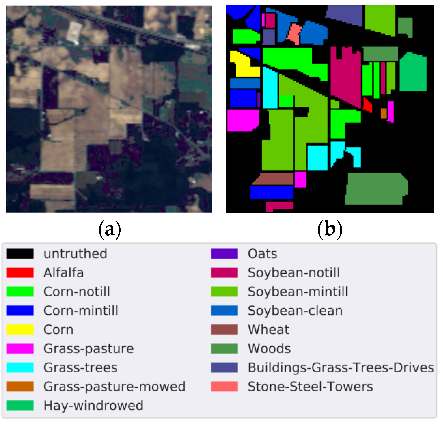
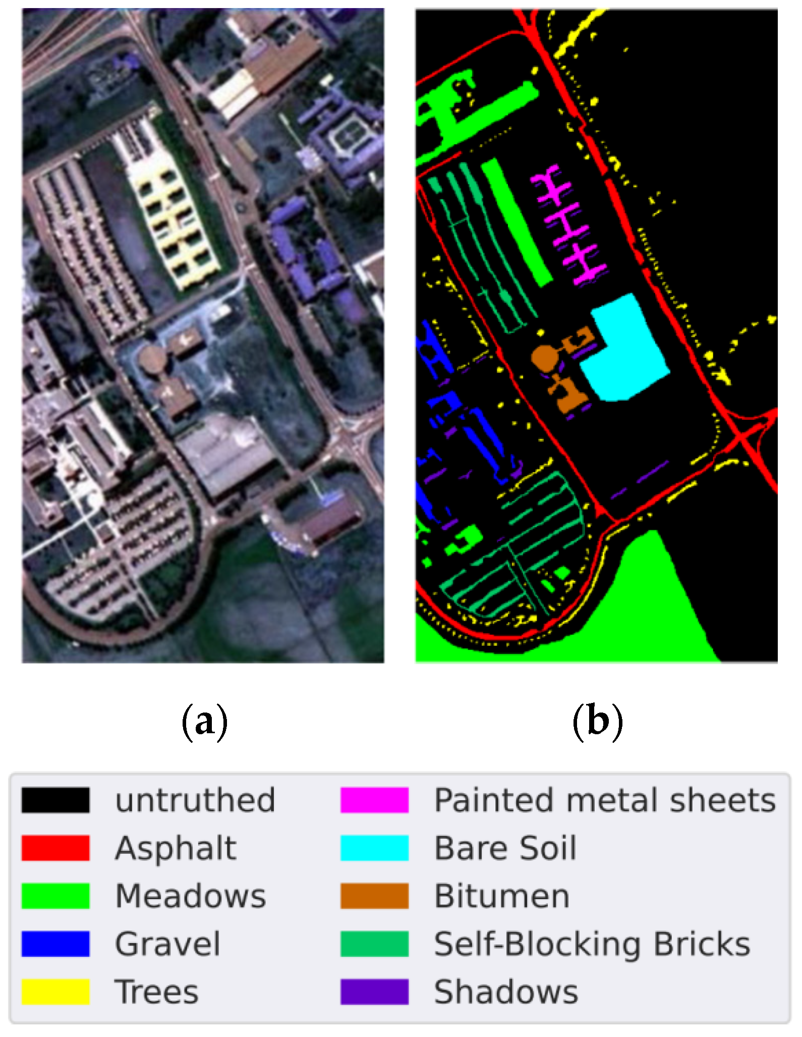
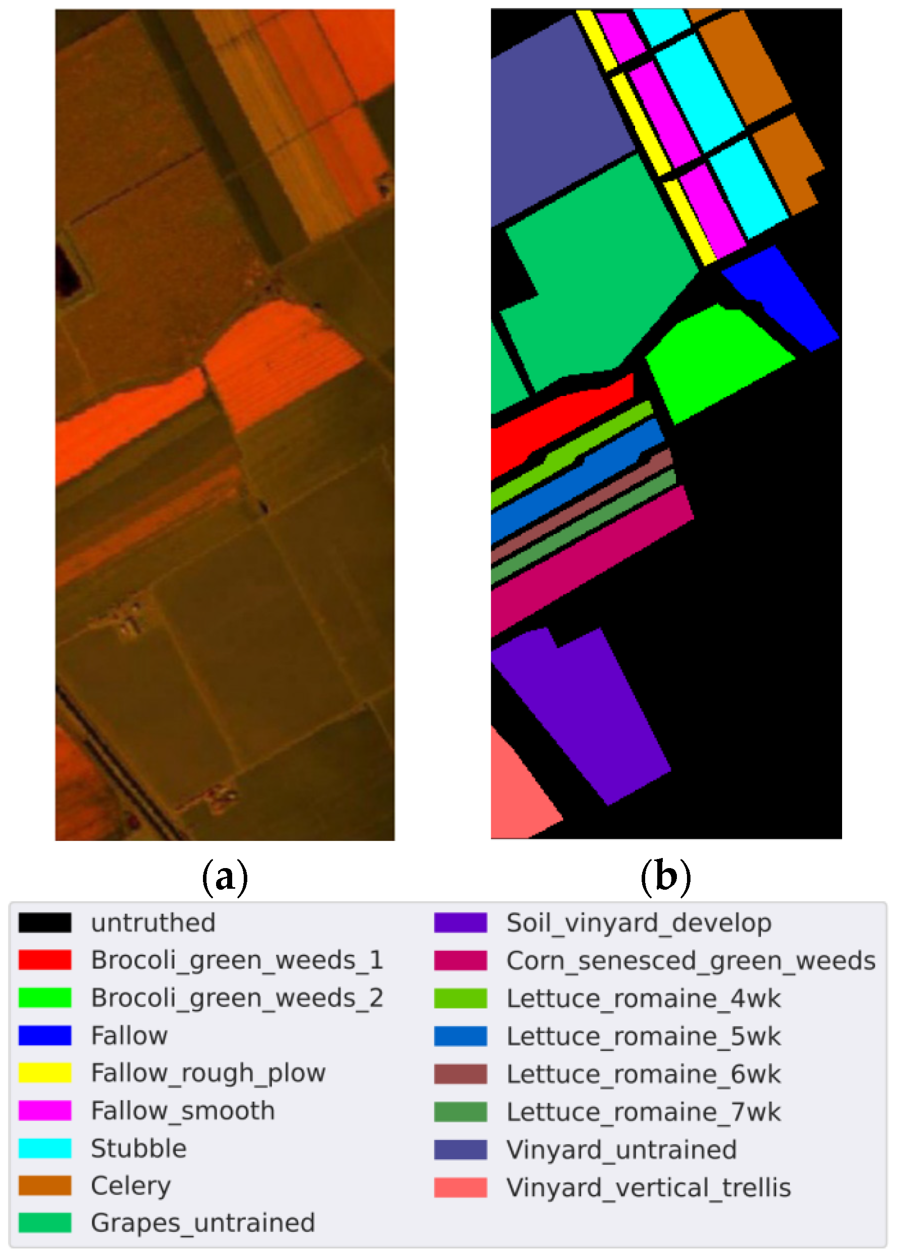
4.1. Data Sets

The Indian Pine (IP) data set which contains 16 classes and 10,249 samples was captured by the Airborne Visible/Infrared Imaging Spectrometer (AVIRIS) sensor in northwestern Indiana. Its spatial size and resolution are 145 × 145 pixels and 20-m per pixel. The number of bands is reduced to 200 by removing bands covering the region of water absorption. The false-color image and corresponding ground-truth map of the IP data set are shown in Figure 4. Table 1 lists the samples of the IP data set.
The Pavia University (PU) data set contains 610 × 340 pixels. It has 103 spectral bands that range from 430 to 860 nm. Its spatial resolution is 1.3-m per pixel. It was collected by the Reflective Optics Spectrographic Image System (ROSIS). It contains nine categories representing different types of land cover. Figure 5 shows the false-color image and corresponding ground-truth map of the PU data set. The samples of the PU data set are listed in Table 2.
The Salinas Scene (SA) data set was gathered by the AVIRIS sensor over Salinas Valley, California. It consists of 145 × 145 pixels with 204 spectral bands that range from 400 to 2500 nm. The data set contains 16 categories of objects, with a total of 54,129 samples. The false-color image and corresponding ground-truth map of the SA data set are shown in Figure 6. Table 3 lists the samples of the SA data set.

4.2. Experimental Setup

In our experiment, we mainly perform the small-sample HSI classification to demonstrate the effectiveness and robustness of the proposed fusion framework. Since HSI contains a rich amount of redundant information, we need to preprocess the HSI data to improve the efficiency of subsequent feature extraction. Accroding to [26], PCA algorithm, which is a commonly used strategy for preprocessing the HSI data, is first employed for the dimensionality reduction in HSI to extract the representative band data. After preprocessing, different handcrafted feature-based and CNN-based methods are utilized for the feature extraction of HSI pixels in the experiment.
At the first set of experiments, our proposed 3D-FHOG is mainly compared with the handcrafted feature-based methods including the original spectral feature, extended multi-attribute profile (EMAP) [51], HOG [31], SIFT [13], 3D-LBP [14], 3D-Gabor [17] and 3D-DWT [18], respectively. In our experiment, SVM [52] is applied to classify the feature vectors of HSI pixels. Then, seven CNN-based methods are considered, i.e., semi-1D CNN [21], 3D FCN [23], semi-3D CNN [24], 3D CNN [25], 1D RNN [22], HybridSN [26] and 3DCSN [43], which are utilized to compare with MDSN and the fusion of 3D-FHOG and MDSN (3D-FHOG + MDSN).
In the training process of MDSN, two phases are included. Firstly, the parameter of our proposed model is updated by Adam optimizer [53] and contrastive loss when per- forming the contrastive learning. Besides, we use an initial learning rate of 5 × 10⁻³, and the weight decay is set to be 0 in contrastive learning phase. In the classification training phase, we use another Adam optimizer and cross-entropy loss to update the parameters of our model. Moreover, the learning rate is set to be 1 × 10⁻³, and the weight decay is set to be 5 × 10⁻⁵ in this phase. According to [43], the input patch size of MDSN is empirically set to be 25 × 25 × 30 for IP and 25 × 25 × 15 for PU and SA, respectively.
In order to compare the classification performance of the above different methods, overall accuracy (OA), average accuracy (AA) and kappa coefficient (κ) are adopted as the evaluation metric. Quantitatively, the greater the values of OA, AA, and κ are, the better the classification result is. Moreover, the classification experiments of each method are repeated 5 times to avoid the accidental phenomenon. Classification accuracy mean and variance of each method are shown in the experimental statistical table.

4.3. Experimental Result and Analysis

In this section, the classification results of different feature extraction methods on three public HSI data sets are analyzed visually and quantitatively.

4.3.1. Influence of the Input Patch Size for 3D-FHOG

First, influence of the input patch size for our proposed 3D-FHOG is examined. Specifically, the size of input patch for 3D-FHOG is set to be 7 × 7 × 7, 9 × 9 × 9, 11 × 11 × 11, 13 × 13 × 13, 15 × 15 × 15 and 17 × 17 × 17 for analysis. Table 4 shows the classification perfor- mance of 3D-FHOG with different input patch sizes on IP data set. It can be concluded that when the size of input patch increases, the values of OA, AA and κ of 3D-FHOG show a trend of increasing first and then decreasing. When input patch size is 15 × 15 × 15, the classification performance of 3D-FHOG is the best. The reason for the decrease in classification performance is the redundant information contained in the local spatial–spectral neighborhood. Therefore, in the following experiment, the input patch size is fixedly set to be 15 × 15 × 15 for 3D-FHOG.

4.3.2. Compared with Handcrafted Feature-Based Methods

In order to verify the effectiveness of 3D-FHOG in small-sample HSI classification, the proposed 3D-FHOG is compared with seven handcrafted feature-based methods. When three labeled samples per class are adopted as the training set, detail classification results with different handcrafted feature-based methods are listed in Table 5, Table 6 and Table 7 for IP, PU and SA data sets, respectively. As observed from Table 5, Table 6 and Table 7, we can make four observations, which are described as follows.
Firstly, compared with the 2D handcrafted feature descriptors, spectral feature and 3D handcrafted feature descriptors can achieve better classification performance. For instance, the OA of 3D-LBP is 15.70% higher than that of HOG on the IP data set. This indicates that only extracting the spatial information will destroy the correlation between spectral bands.
Secondly, the classification performance of 3D handcrafted feature descriptors is always superior to the spectral feature. Because 3D handcrafted feature descriptors can exploit both spatial and spectral information, which makes them more effective in HSI classification.
Thirdly, EMAP feature descriptor shows more excellent classification performance on PU and SA data sets. Since EMAP is based on morphological attribute filters and multi-level analysis, it is suggested that combining the features with different dimensions or scales is an effective solution for small-sample HSI classification.
Finally, by comparing with spectral, 2D handcrafted and 3D handcrafted feature descriptors, we can observe that our proposed 3D-FHOG feature descriptor obtains the best classification results in three public data sets. By integrating with fuzzy logic, 3D-FHOG is able to overcome the local spatial–spectral feature uncertainty and extract more discriminative spatial–spectral features.

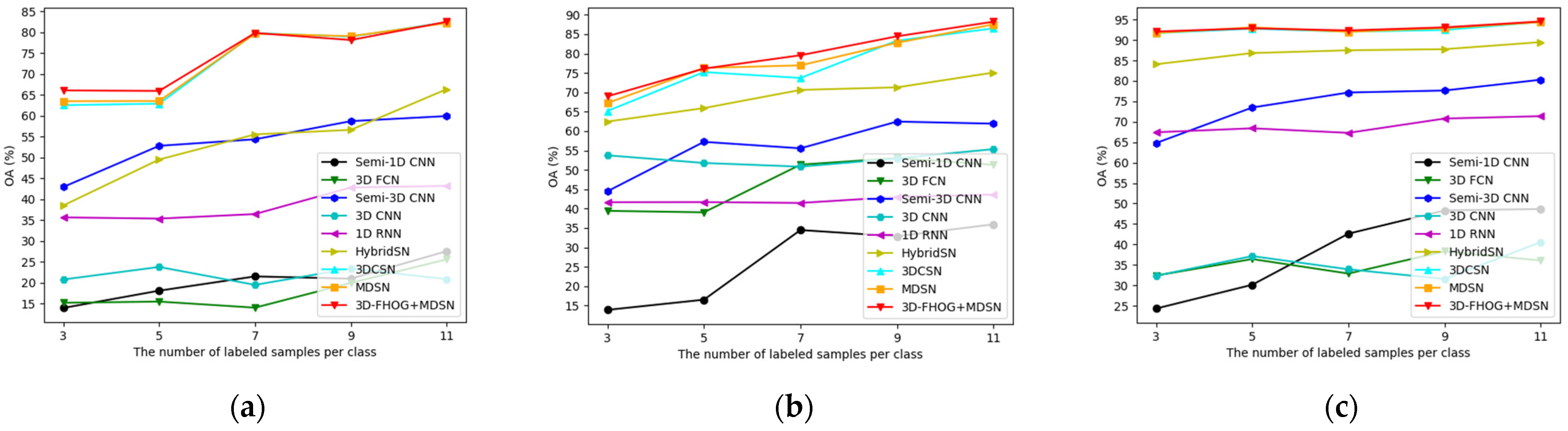
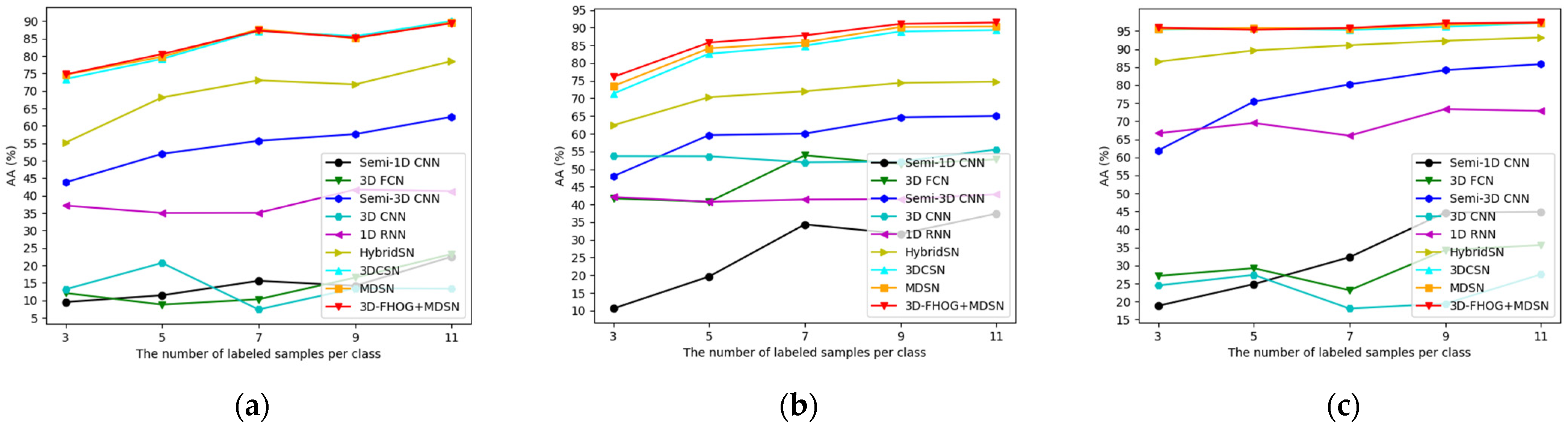
4.3.3. Compared with CNN-Based Methods

To further demonstrate the effectiveness and robustness of the proposed fusion framework, 3D-FHOG + MDSN method is compared with eight representative CNN- based methods. These CNN-based methods include Semi-1D CNN, 3D FCN, Semi-3D CNN, 3D CNN, 1D RNN, HybridSN, 3DCSN and MDSN. Table 8 reports the OA, AA, κ and the classification accuracy of each class for HSI classification with three labeled samples per class on the IP data set. The statistical results suggest that HybridSN, 3DCSN and MDSN methods, which incorporate the multidimensional CNN feature, are superior to the single-dimensional CNN-based methods. Additionally, both Semi-3D CNN and 1D RNN can achieve excellent classification performance. This verifies that 3D CNN combined with semi-supervised learning is effective for small-sample HSI classification, and 1D RNN is able to take full advantage of spectral correlation and band-to-band variability. Moreover, MDSN and 3DCSN, which are based on the learning mechanism of Siamese network, can obtain more accurate results. Especially, 3D-FHOG + MDSN method has the best classification results on the IP data set, which indicates that our proposed fusion framework can fully combine the advantage of multidimensional CNN and handcrafted features.
As for the PU data set, detail classification results with nine different methods are listed in Table 9. As observed in Table 9, the performance of MDSN, 3DCSN and HybridSN is significantly higher than that of the Semi-1D CNN, 3D FCN, Semi-3D CNN, 3D CNN and 1D RNN on the PU data set, which further demonstrates the superiority of multidimensional CNN features and learning mechanism of Siamese network in small- sample HSI classification. Furthermore, 3D-FHOG + MDSN consistently provides the best classification results on PU data set.
With respect to the SA data set, for three labeled samples per class, the OA, AA and κ measure for each class using different approaches are shown in Table 10. From Table 10, it is found that OA and κ of the proposed 3D-FHOG + MDSN are 92.06% and 91.16, respectively, in comparison with the OA and κ of 24.31% and 19.30, 32.38% and 28.11, 64.79% and 60.91, 32.34% and 27.07, 67.42% and 63.99, 84.07% and 82.29, 91.69% and 90.74, 91.72% and 90.78 for Semi-1D CNN, 3D FCN, Semi-3D CNN, 3D CNN, 1D RNN, HybridSN, 3DCSN and MDSN, respectively. The same conclusion can be drawn that classification accuracies obtained by 3D-FHOG + MDSN are better than others, which in turn demonstrates the effectiveness of our proposed fusion framework.

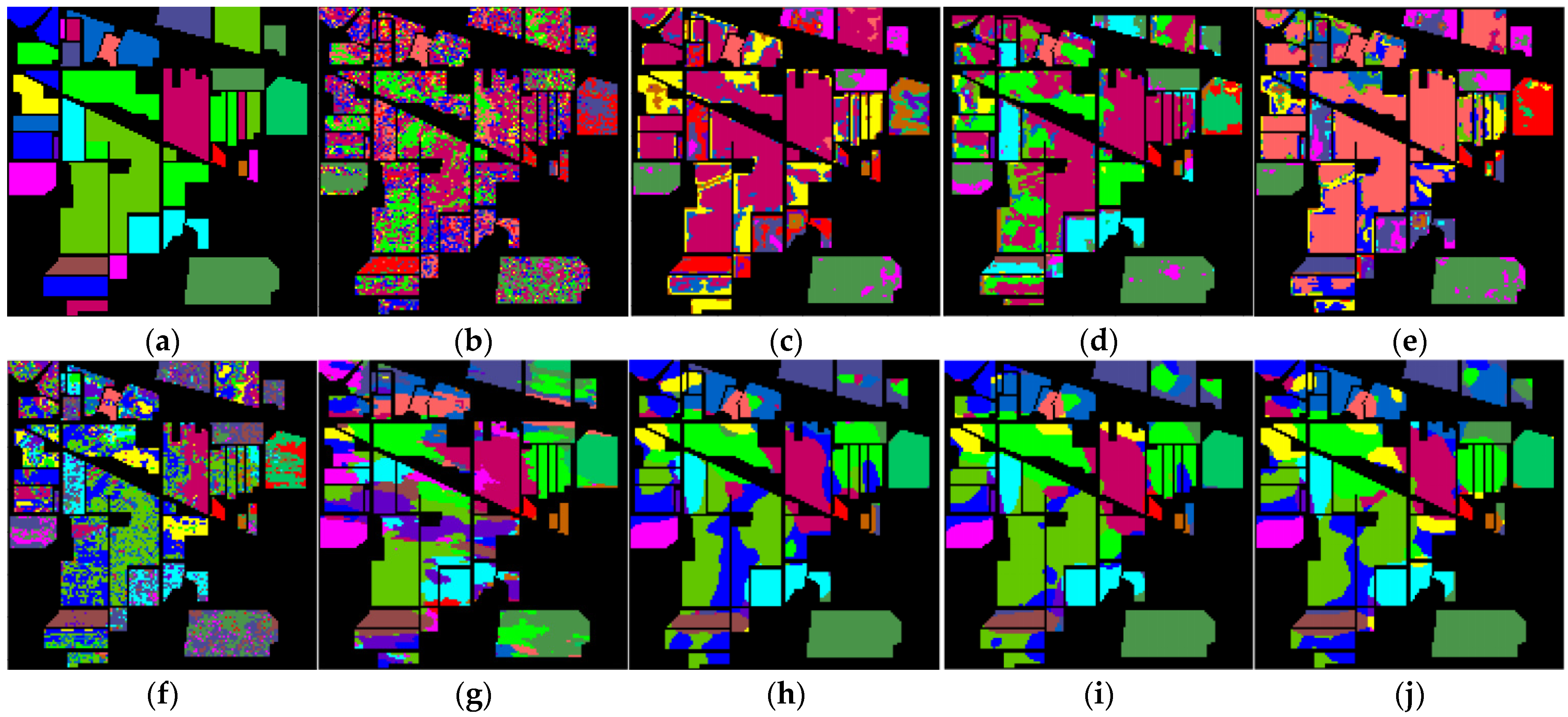
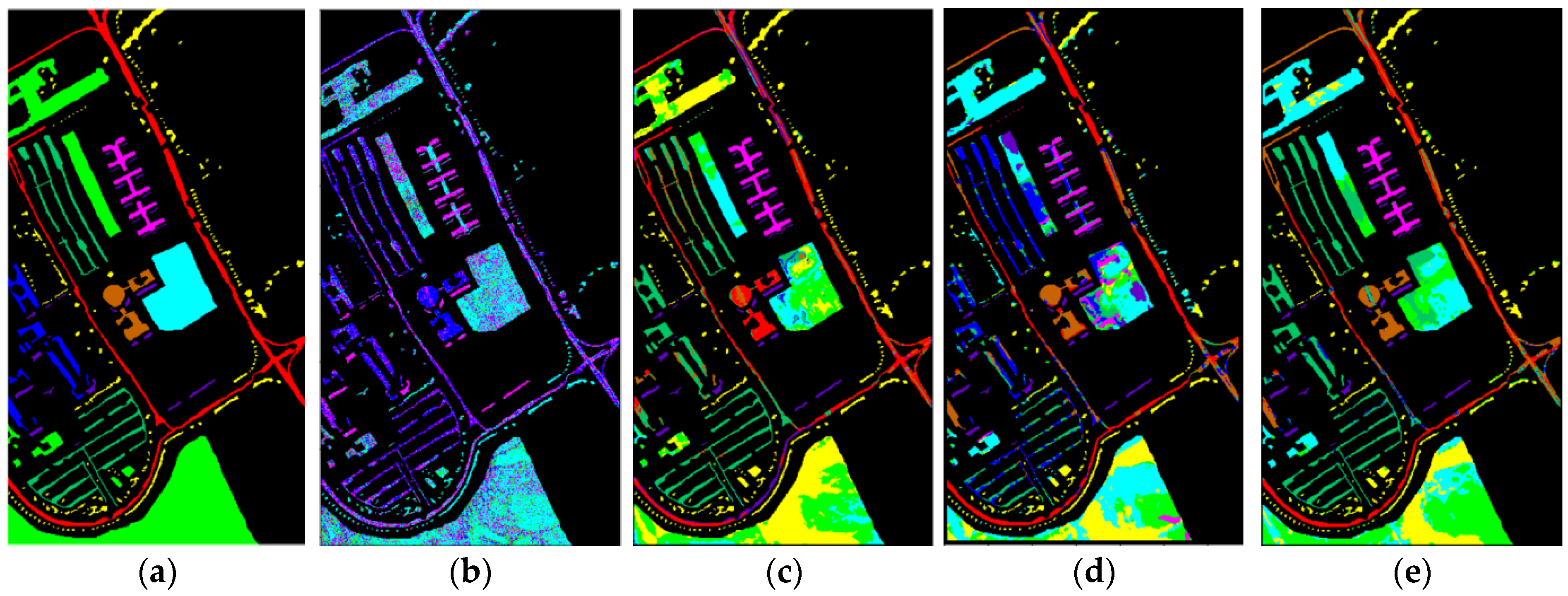
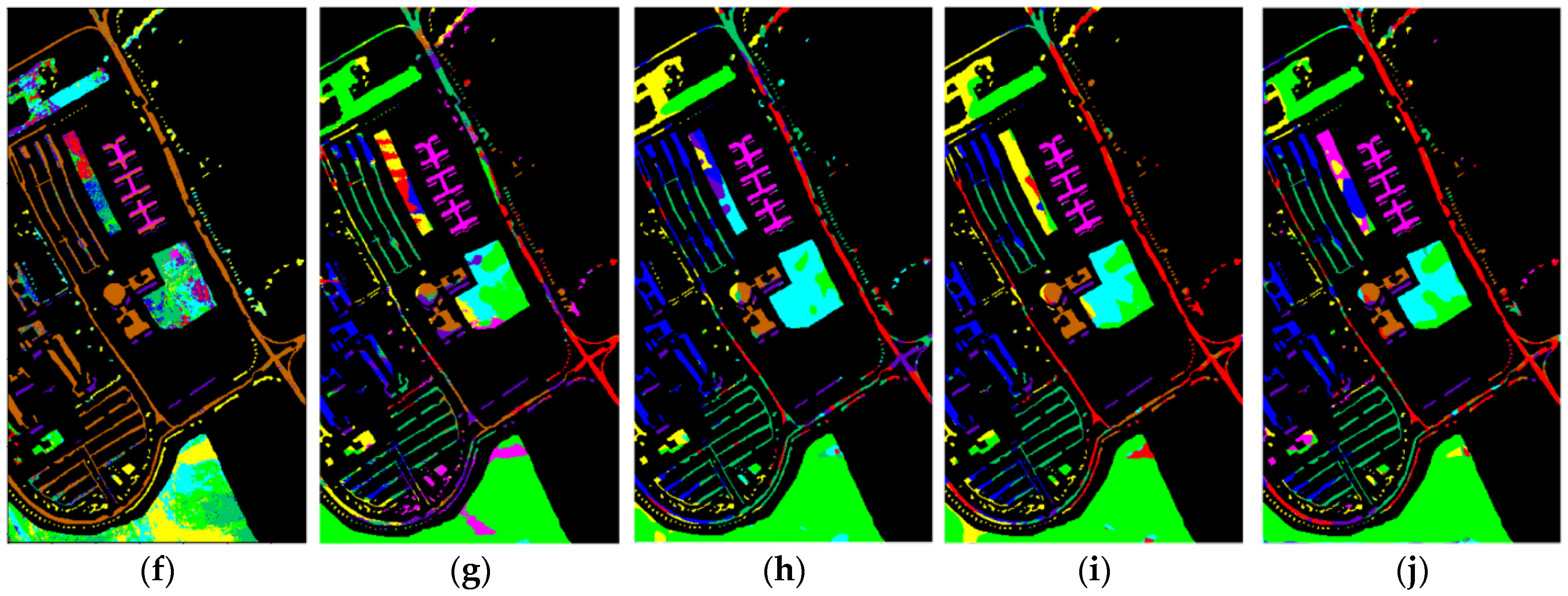
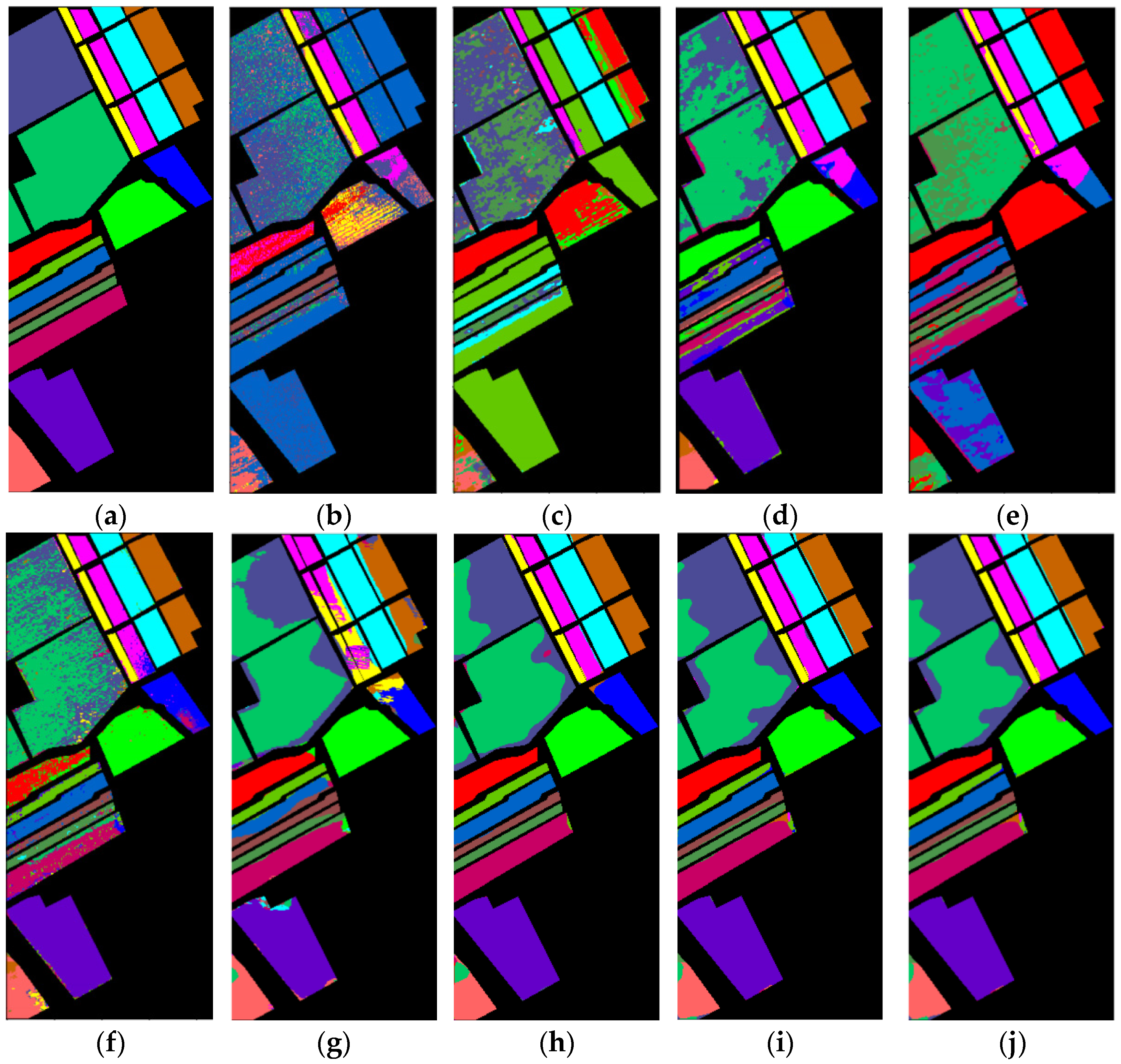
4.3.4. Classification Maps

Furthermore, classification performances of nine different methods are visually investigated on three public HSI data sets. Figure 7 shows the classification maps of Semi-1D CNN, 3D FCN, Semi-3D CNN, 3D CNN, 1D RNN, HybridSN, 3DCSN, MDSN and 3D-FHOG + MDSN on the IP data set with three labeled samples per class. Comparing the classification maps of each method in Figure 7, the maps of HybridSN, 3DCSN, MDSN and 3D-FHOG + MDSN are obviously more similar to the ground map than those of other methods. Especially, the map of 3D-FHOG + MDSN, which effectively combines the multidimensional CNN and handcrafted features, is the most similar. Additionally, the classification maps on the PU data set using nine different methods with three labeled samples per class are shown in Figure 8. It can be seen from Figure 8 that more query samples are obviously assigned to the correct class on the maps of multidimensional CNN-based methods than others, and the map of 3D-FHOG + MDSN is more consistent with the ground-truth map, which indicates that the performance of MDSN is effectively enhanced with the 3D-FHOG feature. In terms of the SA data set, Figure 9 displays the classification maps resulting from nine different methods for the SA data set with three labeled samples per class. The same conclusion can be drawn that the map of 3D-FHOG + MDSN is more similar to the ground-truth map than other methods, which further shows its robustness in small-sample HSI classification.

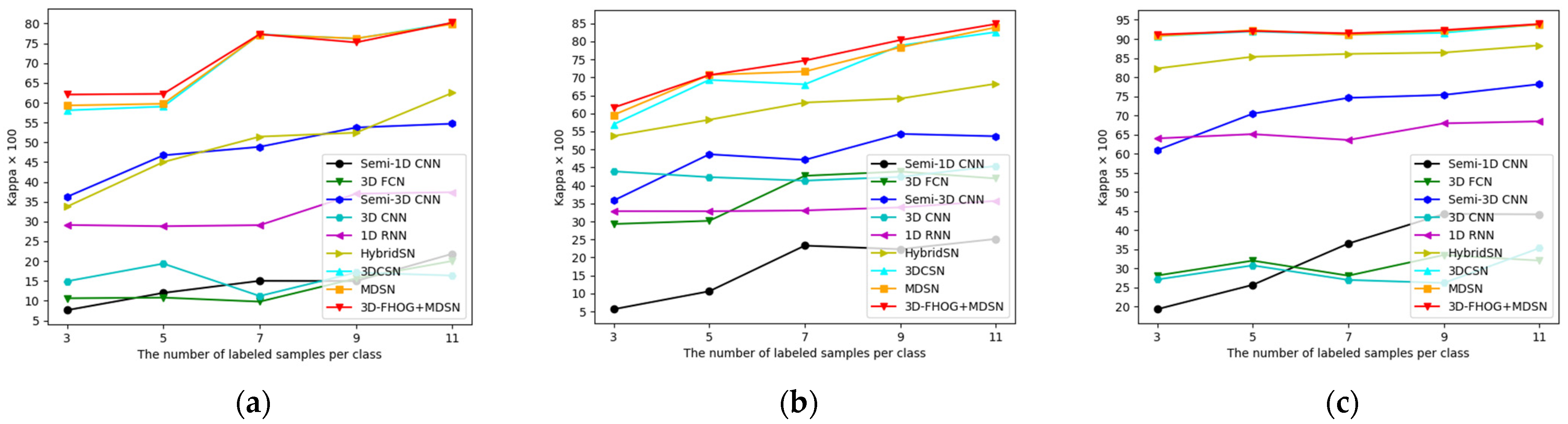
4.3.5. Influence of Training Sample Size

To further illustrate the superiority of 3D-FHOG + MDSN with different numbers of labeled samples, we take 3, 5, 7, 9, and 11 labeled samples for each class to build the training data set. Specifically, we have conducted three groups of experiment on three public HSI data sets. Then, the curve change of nine methods is obtained. It can be seen from Figure 10 that the OA of each method generally rises as the number of labeled samples increases. However, single-dimensional CNN-based methods are unstable in the scenery of small-scale training samples, which may result in the sharp decrease in classification accuracy when the number of labeled samples increases. Especially, the proposed 3D-FHOG + MDSN method outperforms other methods in most cases, which demonstrates its adaptability to the variance of the number of labeled samples. Additionally, Figure 11 and Figure 12 display the AA and κ measure as functions of the number of labeled samples per class. The same conclusion can be drawn that the AA and κ of our proposed 3D-FHOG + MDSN method is always the best in terms of different training sample sizes. Besides, we also find that the gap between the classification accuracy of various methods increases when the number of training samples is fewer. This indicates that the performance of CNN-based method will be enhanced with the increase in labeled samples, which in turns minimizes the contribution of handcrafted features. Meanwhile, incorporating the handcrafted feature with the CNN-based method will not cause a decrease in classification accuracy, but will improve the reliability of classification result. Hence, it is suggested that our proposed 3D-FHOG + MDSN method is more robust and reliable in the scenery of small-scale training samples.
In summary, the performance of MDSN enhanced with 3D-FHOG feature in small-sample HSI classification is better than those of representative handcrafted and CNN-based spatial–spectral feature extraction methods, especially when the training sample size is smaller. This in turn verifies the effectiveness of the proposed fusion framework.

4.3.6. Time Consumption

In this section, the running time of different methods is analyzed to evaluate their computational efficiency. Table 11 reports the running time of different methods on the three HSI data sets with three labeled samples per class. All the experiments are conducted on a computer with an Intel Core i3-4160 processor with 3.6 GHz, 8 GB of DDR3 RAM, an NVIDIA Geforce RTX 1060 graphical processing unit (GPU). For the higher computational cost methods including Semi-1D CNN, 3D FCN and Semi-3D CNN, the processing time is long. In terms of 3D CNN, it has a relatively short training time, but achieves poor classification performance. In addition, for the lightweight networks (i.e., 1D RNN and HybridSN), the running time is short, and these methods can obtain better classification results. Additionally, for the 3DCSN, MDSN and 3D-FHOG+ MDSN, since these methods are based on the idea of Siamese network and composed of CNN blocks with multiple dimensions, more time is consumed by learning the multi- dimensional CNN features from the HSI pixel pairs. Meanwhile, the classification performances of these methods are effectively improved.
Especially, our proposed 3D-FHOG + MDSN contains the additional time of hand- crafted feature extraction (HFE). Table 12 reports the HFE time of 3D-FHOG + MDSN on the three HSI data sets with three labeled samples per class. Note that the HFE time represents the time of HFE for all HSI samples in the data set. Hence, the more samples the data set contains, the more time it takes for 3D-FHOG feature extraction. In some high-sensitive areas, we can spend more time to obtain the more reliable and accurate results. Note that HFE time for each pixel is 0.07s. In real military applications, a military target contained in the HSI is generally composed of about 100 pixels, which only takes 7s for HFE. Therefore, the increase in time is acceptable. To sum up, in terms of some special small-sample HSI classification tasks without considering the computational cost, our proposed method will be an effective solution to achieve more accurate and reliable classification results.

5. Conclusions

In this paper, a fusion framework of multidimensional CNN and handcrafted features is proposed for small-sample HSI classification. Specifically, we design the 3D-FHOG descriptor to extract the handcrafted spatial–spectral feature, which is suggested to be more robust by overcoming the local spatial–spectral feature uncertainty. Then, to further extract the CNN-based spatial–spectral feature, an effective Siamese network, i.e., MDSN is proposed, which can effectively achieve the integration of CNN-based spatial–spectral features from multiple dimensions. Finally, our proposed MDSN combined with 3D-FHOG is employed for small-sample HSI classification to verify the effectiveness of our proposed fusion framework. Experiment results on three public HSI data sets indicate that our proposed MDSN combined with 3D-FHOG is superior to the representative handcrafted and CNN-based spatial–spectral feature extraction methods, which in turn demonstrates the effectiveness of the proposed fusion framework. More importantly, our proposed fusion framework has the advantage of expandability. In the future work, we will continue to explore the more discriminative and efficient spatial–spectral feature extraction methods, and integrate them into our proposed fusion framework, which helps to improve the small-sample HSI classification accuracy.

Author Contributions

Methodology, H.T. and Y.L.; investigation, Z.H., L.Z. and W.X.; resources, Y.L., L.Z. and W.X.; writing—original draft preparation, H.T.; writing—review and editing, H.T.,Y.L. and Z.H.; visualization, H.T. and Z.H.; supervision, Y.L., L.Z. and W.X. All authors have read and agreed to the published version of the manuscript.

Funding

This work was partially supported by National Natural Science Foundation of China (Nos. 61771319, 62076165, 61871154), Natural Science Foundation of Guangdong Province (No. 2019A1515011307), Shenzhen Science and Technology Project (No. JCYJ20180507182259896, No. 20200826154022001) and the Other Project (Nos. 2020KCXTD004, WDZC20195500201).

Data Availability Statement

The IP, PU and SA data sets can be obtained from http://www.ehu.eus/ccwintco/index.php?title=Hyperspectral_Remote_Sensing_Scenes (accessed on 28 June 2022).

Acknowledgments

We would like to thank the authors for providing the data used in this study. We would also like to thank all the professionals for kindly providing the codes associated with the experiments.

Conflicts of Interest

The authors declare no conflict of interest.

References

  1. Chakraborty, T.; Trehan, U. Spectralnet: Exploring spatial-spectral waveletcnn for hyperspectral image classification. arXiv 2021, arXiv:2104.00341. [Google Scholar]
  2. Zhang, Y.; Liu, K.; Dong, Y.; Wu, K.; Hu, X. Semisupervised classification based on SLIC segmentation for hyperspectral image. IEEE Geosci. Remote Sens. Lett. 2019, 17, 1440–1444. [Google Scholar] [CrossRef]
  3. Li, Y.; Tang, H.; Xie, W.; Luo, W. Multidimensional local binary pattern for hyperspectral image classification. IEEE Trans. Geosci. Remote Sens. 2021, 60, 1–13. [Google Scholar] [CrossRef]
  4. Luo, F.; Zou, Z.; Liu, J.; Lin, Z. Dimensionality reduction and classification of hyperspectral image via multistructure unified discriminative embedding. IEEE Trans. Geosci. Remote Sens. 2021, 60, 1–16. [Google Scholar] [CrossRef]
  5. Zhou, Y.; Chen, P.; Liu, N.; Yin, Q.; Zhang, F. Graph-Embedding Balanced Transfer Subspace Learning for Hyperspectral Cross-Scene Classification. IEEE J. Sel. Top. Appl. Earth Observ. Remote Sens. 2022, 15, 2944–2955. [Google Scholar] [CrossRef]
  6. Ye, M.; Qian, Y.; Zhou, J.; Tang, Y. Dictionary learning-based feature-level domain adaptation for cross-scene hyperspectral image classification. IEEE Trans. Geosci. Remote Sens. 2017, 55, 1544–1562. [Google Scholar] [CrossRef] [Green Version]
  7. Mustafa, G.; Zheng, H.; Khan, I.H.; Tian, L.; Jia, H.; Li, G.; Cheng, T.; Tian, Y.; Cao, W.; Zhu, Y.; et al. Hyperspectral Reflectance Proxies to Diagnose In-Field Fusarium Head Blight in Wheat with Machine Learning. Remote Sens. 2022, 14, 2784. [Google Scholar] [CrossRef]
  8. Zhang, N.; Yang, G.; Pan, Y.; Yang, X.; Chen, L.; Zhao, C. A review of advanced technologies and development for hyperspectral-based plant disease detection in the past three decades. Remote Sens. 2020, 12, 3188. [Google Scholar] [CrossRef]
  9. Uzair, M.; Mahmood, A.; Mian, A. Hyperspectral Face Recognition with Spatiospectral Information Fusion and PLS Regression. IEEE Trans. Image Process. 2015, 24, 1127–1137. [Google Scholar] [CrossRef]
  10. Zhang, X.; Zhao, H. Hyperspectral-cube-based mobile face recognition: A comprehensive review. Inf. Fusion 2021, 74, 132–150. [Google Scholar] [CrossRef]
  11. Dobler, G.; Ghandehari, M.; Koonin, S.E.; Sharma, M.S. A hyperspectral survey of New York City lighting technology. Sensors 2016, 16, 2047. [Google Scholar] [CrossRef] [PubMed] [Green Version]
  12. Baur, J.; Dobler, G.; Bianco, F.; Sharma, M.; Karpf, A. Persistent hyperspectral observations of the urban lightscape. In Proceedings of the 2018 IEEE Global Conference on Signal and Information Processing (GlobalSIP), Anaheim, CA, USA, 26–29 November 2018; pp. 983–987. [Google Scholar]
  13. Lowe, D. Distinctive image features from scale-invariant keypoints. Int. J. Comput. Vis. 2004, 60, 91–110. [Google Scholar] [CrossRef]
  14. Ojala, T.; Pietikainen, M.; Maenpaa, T. Multiresolution gray-scale and rotation invariant texture classification with local binary patterns. IEEE Trans. Pattern Anal. Mach. Intell. 2002, 24, 971–987. [Google Scholar] [CrossRef]
  15. Zhao, G.; Pietikainen, M. Dynamic texture recognition using local binary patterns with an application to facial expressions. IEEE Trans. Pattern Anal. Mach. Intell. 2007, 29, 915–928. [Google Scholar] [CrossRef] [Green Version]
  16. Jia, S.; Hu, J.; Zhu, J.; Jia, X.; Li, Q. Three-dimensional local binary patterns for hyperspectral imagery classification. IEEE Trans. Geosci. Remote Sens. 2017, 55, 2399–2413. [Google Scholar] [CrossRef]
  17. He, L.; Li, J.; Plaza, A.; Li, Y. Discriminative Low-Rank Gabor Filtering for Spectral-Spatial Hyperspectral Image Classification. IEEE Trans. Geosci. Remote Sens. 2017, 55, 1381–1395. [Google Scholar] [CrossRef]
  18. Cao, X.; Xu, L.; Meng, D.; Zhao, Q.; Xu, Z. Integration of 3-dimensional discrete wavelet transform and Markov random field for hyperspectral image classification. Neurocomputing 2017, 226, 90–100. [Google Scholar] [CrossRef]
  19. Sharma, V.; Diba, A.; Tuytelaars, T.; Gool, L. Hyperspectral CNN for Image Classification & Band Selection, with Application to Face Recognition; Tech. Rep. KUL/ESAT/PSI/1604; KU Leuven: Leuven, Belgium, 2016. [Google Scholar]
  20. Hu, W.; Huang, Y.; Wei, L.; Zhang, F.; Li, H. Deep convolutional neural networks for hyperspectral image classification. J. Sens. 2015, 2015, 1–12. [Google Scholar] [CrossRef] [Green Version]
  21. Boulch, A.; Audebert, N.; Dubucq, D. Autoencodeurs pour la visualisation d’images hyperspectrales. In Proceedings of the 25th Colloque Gretsi, Juan-les-Pins, France, 5–8 September 2017; pp. 1–4. [Google Scholar]
  22. Mou, L.; Ghamisi, P.; Zhu, X. Deep recurrent neural networks for hyperspectral image classification. IEEE Trans. Geosci. Remote Sens. 2017, 55, 3639–3655. [Google Scholar] [CrossRef] [Green Version]
  23. Lee, H.; Kwon, H. Going deeper with contextual CNN for hyperspectral image classification. IEEE Trans. Image Process. 2017, 26, 4843–4855. [Google Scholar] [CrossRef] [Green Version]
  24. Liu, B.; Yu, X.; Zhang, P.; Tan, X.; Yu, A.; Xue, Z. A semi-supervised convolutional neural network for hyperspectral image classification. Remote Sens. Lett. 2017, 8, 839–848. [Google Scholar] [CrossRef]
  25. Luo, Y.; Zou, J.; Yao, C.; Zhao, X.; Li, T.; Bai, G. HSI-CNN: A novel convolution neural network for hyperspectral image. In Proceedings of the 2018 International Conference on Audio, Language and Image Processing (ICALIP), Shanghai, China, 16–17 July 2018; pp. 464–469. [Google Scholar]
  26. Roy, S.; Krishna, G.; Dubey, S.; Bidyut, B. HybridSN: Exploring 3-D–2-D CNN feature hierarchy for hyperspectral image classification. IEEE Geosci. Remote Sens. Lett. 2019, 17, 277–281. [Google Scholar] [CrossRef] [Green Version]
  27. Rostami, M.; Kolouri, S.; Eaton, E.; Kim, k. Deep transfer learning for few-shot SAR image classification. Remote Sens. 2019, 11, 1374. [Google Scholar] [CrossRef] [Green Version]
  28. Alajaji, D.; Alhichri, H.S.; Ammour, N.; Alajlan, N. Few-shot learning for remote sensing scene classification. In Proceedings of the 2020 Mediterranean and Middle-East Geoscience and Remote Sensing Symposium (M2GARSS), Tunis, Tunisia, 9–11 March 2020; pp. 81–84. [Google Scholar]
  29. Yuan, Z.; Huang, W. Multi-attention DeepEMD for few-shot learning in remote sensing. In Proceedings of the 2020 IEEE 9th Joint International Information Technology and Artificial Intelligence Conference (ITAIC), Chongqing, China, 11–13 December 2020; Volume 9, pp. 1097–1102. [Google Scholar]
  30. Kim, J.; Chi, M. SAFFNet: Self-attention-based feature fusion network for remote sensing few-shot scene classification. Remote Sens. 2021, 13, 2532. [Google Scholar] [CrossRef]
  31. Dalal, N.; Triggs, B. Histograms of oriented gradients for human detection. In Proceedings of the 2005 IEEE Computer Society Conference on Computer Vision and Pattern Recognition, San Diego, CA, USA, 20–25 June 2005; Volume 1, pp. 886–893. [Google Scholar]
  32. Surasak, T.; Takahiro, I.; Cheng, C.; Wang, C.; Sheng, P. Histogram of oriented gradients for human detection in video. In Proceedings of the 2018 5th International Conference on Business and Industrial Research (ICBIR), Bangkok, Thailand, 17–18 May 2018; pp. 172–176. [Google Scholar]
  33. Mao, L.; Xie, M.; Huang, Y.; Zhang, Y. Preceding vehicle detection using histograms of oriented gradients. In Proceedings of the 2010 International Conference on Communications, Circuits and Systems (ICCCAS), Chengdu, China, 28–30 July 2010; pp. 354–358. [Google Scholar]
  34. Qi, S.; Ma, J.; Lin, J.; Li, Y.; Tian, J. Unsupervised Ship Detection Based on Saliency and S-HOG Descriptor from Optical Satellite Images. IEEE Geosci. Remote Sens. Lett. 2015, 12, 1451–1455. [Google Scholar]
  35. Chen, G.; Krzyzak, A.; Xie, W. Hyperspectral face recognition with histogram of oriented gradient features and collaborative representation-based classifier. Multimed. Tools. Appl. 2022, 81, 2299–2310. [Google Scholar] [CrossRef]
  36. Chopra, S.; Hadsell, R.; LeCun, Y. Learning a similarity metric discriminatively, with application to face verification. In Proceedings of the 2005 IEEE Computer Society Conference on Computer Vision and Pattern Recognition, San Diego, CA, USA, 20–25 June 2005; Volume 1, pp. 539–546. [Google Scholar]
  37. Melekhov, I.; Kannala, J.; Rahtu, E. Siamese network features for image matching. In Proceedings of the 2016 23rd International Conference on Pattern Recognition (ICPR), Cancun, Mexico, 4–8 December 2016; pp. 378–383. [Google Scholar]
  38. Tao, R.; Gavves, E.; Smeulders, A. Siamese instance search for tracking. In Proceedings of the IEEE Conference on Computer Vision and Pattern Recognition, Cancun, Mexico, 4–8 December 2016; pp. 1420–1429. [Google Scholar]
  39. Bertinetto, L.; Valmadre, J.; Henriques, J.; Vedaldi, A.; Torr, P. Fully-convolutional siamese networks for object tracking. In Proceedings of the European Conference on Computer Vision, Amsterdam, the Netherlands, 8–16 October 2016; pp. 850–865. [Google Scholar]
  40. Koch, G.; Zemel, R.; Salakhutdinov, R. Siamese neural networks for one-shot image recognition. ICML Deep Learn. Workshop 2015, 2, 1–30. [Google Scholar]
  41. Zhao, S.; Li, W.; Du, Q.; Ran, Q. Hyperspectral classification based on siamese neural network using spectral-spatial feature. In Proceeding of 2018 IEEE International Geoscience and Remote Sensing Symposium (IGARSS), Valencia, Spain, 22–27 July 2018; pp. 2567–2570. [Google Scholar]
  42. Liu, B.; Yu, X.; Zhang, P.; Yu, A.; Fu, Q.; Wei, X. Supervised deep feature extraction for hyperspectral image classification. IEEE Trans. Geosci. Remote Sens. 2017, 56, 1909–1921. [Google Scholar] [CrossRef]
  43. Cao, Z.; Li, X.; Jiang, J.; Zhao, L. 3D convolutional siamese network for few-shot hyperspectral classification. J. Appl. Remote Sens. 2020, 14, 048504. [Google Scholar] [CrossRef]
  44. Zeiler, M.; Fergus, R. Visualizing and understanding convolutional networks. In Proceedings of the European Conference on Computer Vision, Zurich, Switzerland, 5–12 September 2014; pp. 818–833. [Google Scholar]
  45. Wold, S.; Esbensen, K.; Geladi, P. Principal component analysis. Chemom. Intell. Lab. Syst. 1987, 2, 37–52. [Google Scholar] [CrossRef]
  46. Zadeh, L. Fuzzy set theory. Inf. Control. 1965, 8, 338–353. [Google Scholar] [CrossRef] [Green Version]
  47. Guo, H.; Zhang, X. A Track-to-Track Association Algorithm Based on Fuzzy Synthetical Function and Its Application. Syst. Eng. Electron. 2003, 25, 1401–1403. [Google Scholar]
  48. Liu, J.; Li, R.; Liu, Y.; Zhang, Z. Multi-sensor data fusion based on correlation function and fuzzy integration function. Syst. Eng. Electron. 2006, 28, 1006–1009. [Google Scholar]
  49. Snell, J.; Swersky, K.; Zemel, R. Prototypical networks for few-shot learning. Adv. Neural Inf. Processing Syst. 2017, 30, 1–11. [Google Scholar]
  50. Tang, H.; Li, Y.; Han, X.; Huang, Q.; Xie, W. A spatial–spectral prototypical network for hyperspectral remote sensing image. IEEE Geosci. Remote Sens. Lett. 2019, 17, 167–171. [Google Scholar] [CrossRef]
  51. Mura, M.; Benediktsson, J.; Waske, B.; Bruzzone, L. Extended profiles with morphological attribute filters for the analysis of hyperspectral data. Int. J. Remote Sens. 2010, 31, 5975–5991. [Google Scholar] [CrossRef]
  52. Melgani, F.; Bruzzone, L. Classification of hyperspectral remote sensing images with support vector machines. IEEE Trans. Geosci. Remote Sens. 2004, 42, 1778–1790. [Google Scholar] [CrossRef] [Green Version]
  53. Kingma, D.P.; Ba, J. Adam: A method for stochastic optimization. arXiv 2014, arXiv:1412.6980. [Google Scholar]
Figure 1. The fusion framework of multidimensional CNN and handcrafted features for small-sample HSI classification. Initially, 3D-FHOG is adopted as the handcrafted feature extraction method, and MDSN is utilized for multidimensional CNN-based feature extraction.
Remotesensing 14 03796 g001
Figure 2. The schematic of 3D-FHOG feature extraction.
Remotesensing 14 03796 g002
Figure 3. The structure of MDSN. Each convolutional block contains a convolutional layer, a batch normalization layer and a ReLU nonlinearity corresponding to its convolutional dimension. When performing the contrastive learning, two different patches are adopted at the same time. In the classification phase, only one patch is used.
Remotesensing 14 03796 g003
Figure 4. IP data set. (a) False-color image. (b) Ground-truth map.
Remotesensing 14 03796 g004
Figure 5. PU data set. (a) False-color image. (b) Ground-truth map.
Remotesensing 14 03796 g005
Figure 6. SA data set. (a) False-color image. (b) Ground-truth map.
Remotesensing 14 03796 g006
Figure 7. Classification maps resulting from nine different methods for the IP data set with three labeled samples per class. (a) Ground-truth. (b) Semi-1D CNN (16.32%). (c) 3D FCN (21.79%). (d) Semi-3D CNN (41.64%). (e) 3D CNN (17.78%). (f) 1D RNN (34.37%). (g) HybridSN (47.51%). (h) 3DCSN (61.20%). (i) MDSN (63.51%). (j) 3D-FHOG + MDSN (66.42%).
Remotesensing 14 03796 g007
Figure 8. Classification maps resulting from nine different methods for the PU data set with three labeled samples per class. (a) Ground-truth. (b) Semi-1D CNN (18.25%). (c) 3D FCN (50.48%). (d) Semi-3D CNN (35.54%). (e) 3D CNN (52.10%). (f) 1D RNN (28.85%). (g) HybridSN (64.06%). (h) 3DCSN (65.08%). (i) MDSN (68.39%). (j) 3D-FHOG + MDSN (73.29%).
Remotesensing 14 03796 g008aRemotesensing 14 03796 g008b
Figure 9. Classification maps resulting from nine different methods for the SA data set with three labeled samples per class. (a) Ground-truth. (b) Semi-1D CNN (26.94%). (c) 3D FCN (28.18%). (d) Semi-3D CNN (72.80%). (e) 3D CNN (42.56%). (f) 1D RNN (80.14%). (g) HybridSN (82.34%). (h) 3DCSN (91.30%). (i) MDSN (91.93%). (j) 3D-FHOG + MDSN (93.25%).
Remotesensing 14 03796 g009
Figure 10. OA as functions of the number of labeled samples per class on three test data sets: (a) IP data set; (b) PU data set; (c) SA data set.
Remotesensing 14 03796 g010
Figure 11. AA as functions of the number of labeled samples per class on three test data sets: (a) IP data set; (b) PU data set; (c) SA data set.
Remotesensing 14 03796 g011
Figure 12. Kappa coefficient as functions of the number of labeled samples per class on three test data sets: (a) IP data set; (b) PU data set; (c) SA data set.
Remotesensing 14 03796 g012
Table 1. Land cover classes and the numbers of samples in the IP data set.
ClassNameSamplesTraining SamplesTesting Samples
1Alfalfa46343
2Corn-notill142831425
3Corn-mintill8303827
4Corn2373234
5Grass-pasture4833480
6Grass-trees7303727
7Grass-pasture-mowed28325
8Hay-windrowed4783475
9Oats20317
10Soybean-notill9723969
11Soybean-mintill245532452
12Soybean-clean5933590
13Wheat2053202
14Woods126531262
15Buildings-Grass-Trees-Drives3863383
16Stone-Steel-Towers93390
Total10,2494810,201
Table 2. Land cover classes and the numbers of samples in the PU data set.
ClassNameSamplesTraining SamplesTesting Samples
1Asphalt663136628
2Meadows18,649318,646
3Gravel209932096
4Trees306433061
5Sheets134531342
6Bare soil502935026
7Bitumen133031327
8Bricks368233679
9Shadow9473944
Total42,7762742,749
Table 3. Land cover classes and the numbers of samples in the SA data set.
ClassNameSamplesTraining SamplesTesting Samples
1Brocoli_green_weeds_1200932006
2Brocoli_green_weeds_2372633723
3Fallow197631973
4Fallow_rough_plow139431391
5Fallow_smooth267832675
6Stubble395933956
7Celery357933576
8Grapes_untrained11,271311,268
9Soil_vinyard_develop620336200
10Corn_senesced_green_weeds327833275
11Lettuce_romaine_4wk106831065
12Lettuce_romaine_5wk192731924
13Lettuce_romaine_6wk9163913
14Lettuce_romaine_7wk107031067
15Vinyard_untrained726837265
16Vinyard_vertical_trellis180731804
Total54,1294854,081
Table 4. Classification performance of 3D-FHOG with different input patch sizes on IP data set.
Input Patch Size7 × 7 × 79 × 9 × 911 × 11 × 1113 × 13 × 1315 × 15 × 1517 × 17 × 17
Evaluation Metric
OA36.30 ± 0.1539.70 ± 0.0442.66 ± 0.0348.71 ± 0.0251.89 ± 0.0150.97 ± 0.01
AA42.27 ± 0.0746.56 ± 0.0549.23 ± 0.0954.23 ± 0.0957.61 ± 0.0557.12 ± 0.06
κ28.49 ± 0.1732.39 ± 0.0535.70 ± 0.0442.02 ± 0.0345.71 ± 0.0144.81 ± 0.01
Table 5. Classification results (%) for Spectral, EMAP, HOG, SIFT, 3D-LBP, 3D-Gabor, 3D-DWT, and 3D-FHOG on the test set of IP data set, with three labeled samples per class as training set.
ClassSpectralEMAPHOGSIFT3D-LBP3D-Gabor3D-DWT3D-FHOG
MeanVarMeanVarMeanVarMeanVarMeanVarMeanVarMeanVarMeanVar
178.602.0473.024.2967.444.8299.530.01100.000.0036.282.9159.536.7073.953.19
224.600.5911.842.1520.390.3131.902.0027.372.0739.263.5923.242.2428.690.40
321.692.5934.323.4217.340.6825.921.2223.700.8524.931.5423.433.3023.531.15
420.852.7033.850.9123.420.1655.471.5744.878.2537.265.1125.300.3831.540.95
540.924.5434.084.1036.540.6736.751.7215.120.5019.465.7112.798.1858.420.30
627.541.4169.521.3636.731.7954.224.0749.570.9229.322.9149.902.5267.980.94
793.600.0589.600.3766.403.11100.000.00100.000.00100.000.0076.000.8872.004.35
849.392.3338.191.1328.211.0564.212.8771.622.7491.960.1366.904.3863.493.59
971.760.7664.700.6987.381.34100.000.00100.000.0075.291.80100.000.0094.441.23
1037.211.1236.624.7321.630.2132.574.6134.083.9317.877.0450.182.1646.810.92
1132.281.4637.754.1814.690.2117.350.9426.665.4826.3210.7318.673.2867.110.16
1212.272.3111.970.3819.560.2424.541.9631.931.1214.811.4622.852.5328.951.45
1394.360.1892.970.3067.031.3873.663.3896.440.0975.740.5153.1711.9674.261.71
1459.305.3059.499.2318.490.2945.918.8062.981.6167.848.3388.732.7463.722.45
1512.640.6328.411.3628.820.7557.182.3236.551.9127.360.6112.740.4946.421.74
1682.001.1691.110.0750.673.1186.672.0396.440.3993.330.4481.330.4980.442.62
OA34.950.0838.500.5122.900.0235.980.1538.600.2136.800.3237.410.1651.890.01
AA47.440.0550.460.0737.800.0556.620.1457.330.0548.570.0547.800.0957.610.05
κ27.480.0731.790.4615.820.0129.280.1733.770.2029.890.2430.680.1845.710.01
Table 6. Classification results (%) for Spectral, EMAP, HOG, SIFT, 3D-LBP, 3D-Gabor, 3D-DWT, and 3D-FHOG on the test set of PU data set, with three labeled samples per class as training set.
ClassSpectralEMAPHOGSIFT3D-LBP3D-Gabor3D-DWT3D-FHOG
MeanVarMeanVarMeanVarMeanVarMeanVarMeanVarMeanVarMeanVar
138.9710.2449.720.9024.342.0356.901.9135.2613.0317.061.9334.063.0558.950.83
230.8210.0744.824.4621.170.1824.074.5844.3811.1829.502.8246.163.5144.843.00
331.140.6473.390.7638.271.6029.370.9550.136.8725.535.4576.811.2571.871.47
475.482.3076.670.7454.130.6628.353.0749.637.5556.374.4596.490.0175.510.76
571.470.0899.150.0055.752.1164.592.9493.020.3499.400.01100.000.0077.031.48
640.1711.7057.734.5126.430.7933.971.4854.912.9577.592.6844.169.6749.712.76
788.450.8169.153.6330.251.0225.640.6282.140.5680.471.0277.2710.0379.743.67
873.110.3932.062.0657.730.4731.222.6485.671.1250.433.9422.230.6979.361.28
999.890.0095.050.0585.930.4843.282.2730.953.6633.116.8865.420.9376.520.94
OA44.630.6353.250.8031.420.0233.250.4350.823.4940.610.6450.180.4256.890.57
AA61.060.1866.410.1443.780.0337.490.0858.460.4252.160.1162.510.0968.170.20
κ35.290.4244.50.7321.640.0221.200.1142.523.1231.160.5140.260.3348.130.56
Table 7. Classification results (%) for Spectral, EMAP, HOG, SIFT, 3D-LBP, 3D-Gabor, 3D-DWT, and 3D-FHOG on the test set of SA data set, with three labeled samples per class as training set.
ClassSpectralEMAPHOGSIFT3D-LBP3D-Gabor3D-DWT3D-FHOG
MeanVarMeanVarMeanVarMeanVarMeanVarMeanVarMeanVarMeanVar
198.280.0297.900.0549.290.8441.400.7857.4310.0668.3211.1895.650.0596.960.08
270.204.3296.100.1436.370.7637.824.4863.120.6476.937.9185.010.1292.460.34
349.980.4076.342.2631.421.2126.342.7249.494.1821.281.0050.857.7593.360.68
498.130.0292.380.3469.891.8985.740.7395.870.0177.946.1497.440.0184.022.35
597.700.0081.144.4450.312.7731.502.2593.810.0560.265.9479.5810.3278.658.17
696.670.0299.590.0050.691.7651.692.3056.1510.4290.360.0277.5017.5897.560.04
797.750.0599.610.0040.751.0718.790.2385.700.0532.386.3264.801.6895.220.05
845.401.8644.124.2625.961.0528.6910.4239.3110.0032.2611.4946.1813.0168.290.41
975.467.8790.751.6435.711.0414.990.7175.413.0797.640.0175.3417.42100.000.01
1029.346.4063.813.4836.714.0218.041.0964.051.0622.004.3225.956.8664.185.06
1177.350.1880.022.1463.833.2789.560.0692.600.0061.677.0978.334.8476.732.54
1273.790.4075.551.7962.853.8760.579.1661.2313.0954.074.0665.971.2081.050.43
1395.640.3676.123.0064.822.1339.016.7236.1716.4295.440.0689.180.0289.350.90
1476.943.9175.356.2375.002.5777.560.7674.131.3162.3810.5466.641.6682.192.28
1566.342.4973.113.6818.790.4345.6610.2677.791.1263.148.1040.548.4138.671.68
1620.450.9572.661.5726.531.4624.700.9841.354.8852.930.3721.444.0057.350.66
OA67.960.1976.030.1437.370.0235.740.1763.780.1857.820.1060.350.7176.950.03
AA73.090.0580.910.1646.180.0943.250.0666.480.1660.560.1266.270.5480.940.08
κ64.590.2373.510.1631.490.0429.700.1460.140.1953.640.1056.350.8474.460.04
Table 8. Classification results (%) for eight different CNN-based methods and 3D-FHOG + MDSN on the test set of IP data set, with three labeled samples per class as training set.
ClassSemi-1D CNN3D FCNSemi-3D CNN3D CNN1D RNNHybridSN3DCSNMDSN3D-FHOG
+MDSN
MeanVarMeanVarMeanVarMeanVarMeanVarMeanVarMeanVarMeanVarMeanVar
13.220.094.740.2242.142.707.800.5724.691.0073.491.35100.000.00100.000.0099.530.01
26.360.684.960.5528.221.2110.851.9824.710.2219.871.1446.290.0353.380.2251.210.10
38.330.9510.881.5820.130.485.090.4023.730.5227.640.6553.011.4959.540.1963.410.22
43.810.1112.170.7922.930.8612.161.0018.540.7017.610.8050.600.5457.520.3855.130.52
511.332.966.911.2042.580.3315.321.1546.470.1558.461.5555.500.0454.580.0257.540.02
67.142.043.030.2969.210.9415.004.0155.142.0070.842.3488.090.2190.760.0291.770.02
77.990.494.000.0540.292.390.750.0229.691.08100.000.00100.000.00100.000.00100.000.00
88.800.697.492.2478.912.9515.479.5763.073.3789.390.1999.120.0298.360.0199.490.00
92.140.034.660.0625.820.294.670.3423.853.7595.290.33100.000.00100.000.00100.000.00
105.870.5211.501.4232.520.138.412.3429.130.4424.993.5958.390.1358.020.1059.860.09
1125.222.8310.574.4738.193.3820.453.5226.451.5917.191.9949.350.6345.530.1153.600.08
129.830.715.140.3120.000.077.791.4517.440.1830.611.0060.100.3155.050.2762.140.02
1324.442.9218.831.9365.110.2625.527.2365.462.4981.887.6281.780.8787.230.1183.560.16
147.161.5934.8413.1774.911.3246.2814.5066.190.3465.550.3883.000.3585.480.2285.860.25
159.030.467.720.6524.920.238.040.6827.610.4550.392.9276.600.0076.660.0076.760.00
1611.644.4046.296.6574.713.117.090.2352.402.5759.560.9272.670.0572.000.1655.560.05
OA13.980.2515.221.6842.950.1220.801.0235.670.1038.520.5062.550.0663.510.0166.080.00
AA9.520.0612.110.5843.790.0413.170.6937.160.1555.170.2573.400.0274.630.0074.720.01
κ7.620.1210.621.0736.230.0814.920.8429.130.0833.760.4558.090.0759.320.0162.070.00
Table 9. Classification results (%) for eight different CNN-based methods and 3D-FHOG + MDSN on the test set of PU data set, with three labeled samples per class as training set.
ClassSemi-1D CNN3D FCNSemi-3D CNN3D CNN1D RNNHybridSN3DCSNMDSN3D-FHOG
+MDSN
MeanVarMeanVarMeanVarMeanVarMeanVarMeanVarMeanVarMeanVarMeanVar
11.000.0233.054.8561.661.8075.390.3142.339.4253.591.1752.580.5063.630.3567.440.24
211.900.8639.225.4941.144.9755.241.3744.651.3567.382.7065.480.2763.510.3364.010.23
311.071.0518.401.3533.010.2717.021.8619.475.4876.121.2287.970.7887.360.2789.830.11
411.931.0449.641.6641.050.8748.315.9158.790.5418.630.1134.451.9337.840.5641.800.58
523.688.9780.476.0773.992.6899.390.0073.572.84100.000.0099.730.0099.970.0099.790.00
610.741.7434.570.0634.790.1736.200.0925.790.0377.960.9274.462.0778.120.8679.320.81
713.052.1226.461.9033.640.7822.893.0321.710.8574.351.3394.060.5291.940.5497.660.08
810.353.3232.580.5650.490.7430.978.6038.205.4147.121.7861.660.2069.220.3470.550.20
91.550.0461.0411.4362.021.8497.490.0854.681.1946.461.2671.480.1869.560.0674.020.11
OA13.880.3239.430.6044.470.4253.760.5441.660.7262.460.5965.180.0967.230.1168.970.09
AA10.580.0441.710.3047.980.1353.660.3942.130.3762.400.1071.320.0873.460.0376.050.04
κ5.630.0629.300.4635.810.2443.910.5732.860.6253.730.6156.970.1259.580.1361.620.11
Table 10. Classification results (%) for eight different CNN-based methods and 3D-FHOG + MDSN on the test set of SA data set, with three labeled samples per class as training set.
ClassSemi-1D CNN3D FCNSemi-3D CNN3D CNN1D RNNHybridSN3DCSNMDSN3D-FHOG
+MDSN
MeanVarMeanVarMeanVarMeanVarMeanVarMeanVarMeanVarMeanVarMeanVar
10.000.0027.605.4929.385.7719.722.5944.335.1098.990.0199.970.0099.790.0099.780.00
221.463.4634.094.3032.7612.2821.446.9038.6313.5698.300.0899.400.0099.300.0199.540.00
313.731.402.150.1151.791.218.150.6946.956.7881.881.0199.830.0099.910.0199.940.00
430.4510.0060.9912.4692.240.3432.0810.3791.740.1266.777.5199.150.0099.080.0199.610.00
514.057.9016.523.6868.873.2028.8711.0258.3915.6857.704.9994.880.3494.490.1595.240.16
630.008.6365.669.9498.600.0076.073.4298.960.0099.420.0098.590.0299.140.0199.670.00
726.157.928.122.6493.310.030.030.0093.070.2296.260.1098.900.0199.080.0199.500.00
812.545.7611.912.2560.373.6730.077.5059.363.6076.190.8585.970.0184.860.0384.470.02
933.276.8129.997.4581.870.3441.3713.0672.4313.3795.950.0996.610.2197.120.2699.300.01
1010.730.908.200.7538.280.3915.784.9858.195.0387.660.1395.470.0294.540.0294.520.01
112.130.1827.215.4237.030.6810.972.4936.126.1197.390.0199.660.0099.590.0099.910.00
1230.116.4031.572.5060.3711.1723.355.0272.697.1380.830.4098.340.0298.400.0298.110.01
1315.411.8817.414.8180.121.2642.658.3389.820.5495.600.6799.870.0099.960.0099.960.00
1441.5713.9313.520.1370.734.3426.7210.9686.540.3887.521.6998.670.0098.740.0199.020.00
156.360.9634.873.7644.372.952.280.2039.593.9965.972.8071.670.2972.730.5272.820.45
1613.111.0043.960.2149.946.5411.814.4879.970.1597.550.1090.300.4293.100.2293.720.11
OA24.310.4032.380.4564.790.0832.342.5267.420.3484.070.0191.690.0091.720.0192.060.01
AA18.820.3627.110.0861.880.2324.462.0366.670.4886.500.0295.450.0195.610.0095.940.01
κ19.300.3228.110.3460.910.1027.072.4863.990.3882.290.0190.740.0090.780.0191.160.01
Table 11. Running time of different methods on the three HSI data sets with three labeled samples per class.
ModelSemi-1D CNN3D FCNSemi-3D CNN3D CNN1D RNNHybridSN3D CSNMDSN3D-FHOG + MDSN
IPTraining Time (s)449.72197.29500.1021.569.764.09295.81314.16314.17
Testing time (s)0.4415.043.914.811.4610.3610.5812.5815.50
PUTraining Time (s)3659.20735.333710.1537.5023.031.7734.6438.6638.58
Testing time (s)3.53140.0123.2219.217.8819.9820.4626.5841.78
SATraining Time (s)2443.70990.522893.4595.2739.322.18102.17114.46115.28
Testing time (s)2.3783.3629.1827.517.7824.9125.5434.9364.84
Table 12. Handcrafted feature extraction (HFE) time of 3D-FHOG + MDSN on the three HSI data sets with three labeled samples per class.
Model3D-FHOG + MDSN
IPHFE time (s)722.57
HFE time for each pixel (s)0.07
PUHFE time (s)3040.99
HFE time for each pixel (s)0.07
SAHFE time (s)3815.43
HFE time for each pixel (s)0.07
Publisher’s Note: MDPI stays neutral with regard to jurisdictional claims in published maps and institutional affiliations.

