
A Spatial–Spectral Combination Method for Hyperspectral Band Selection

Abstract
:1. Introduction
- (1)
- Subspace division is proposed to partition the hyperspectral image cube into multiple groups in space. The bands of high similarity in spectral dimension are assigned into one group. Seven algorithms are proposed. It is shown through a comprehensive comparison that the means algorithm is the most suitable, with the computation time being the shortest.
- (2)
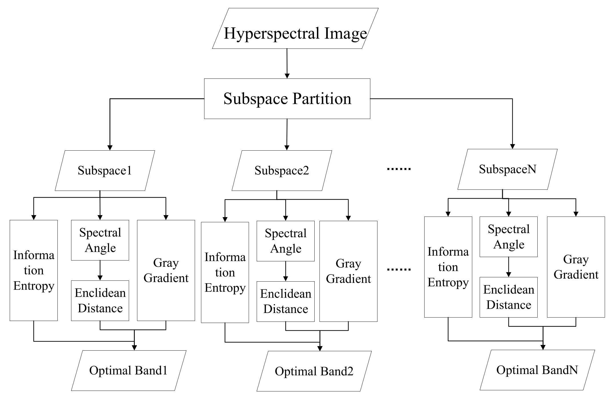
- In each subspace, a spatial–spectral combination method is proposed. The band with maximum information and more prominent characteristics between different categories is selected. Compared with most existing methods about selecting representative band, this method can better exploit the spatial and spectral characteristics. The obtained band subset has more discriminative bands simultaneously.
- (3)
- An automatic method to determine the number of appropriate bands is proposed, which can better evaluate the information redundancy of band set. Experiments show that this algorithm can offer a promising estimation of band number for various date sets.
- (4)
- This method is an unsupervised band selection that does not require any label data.
2. Proposed Approach
2.1. Subspace Partition
2.1.1. Means Method
2.1.2. Correlation-Based Method
- (1)
- Convert a two-dimensional band image into one-dimensional band vector;
- (2)
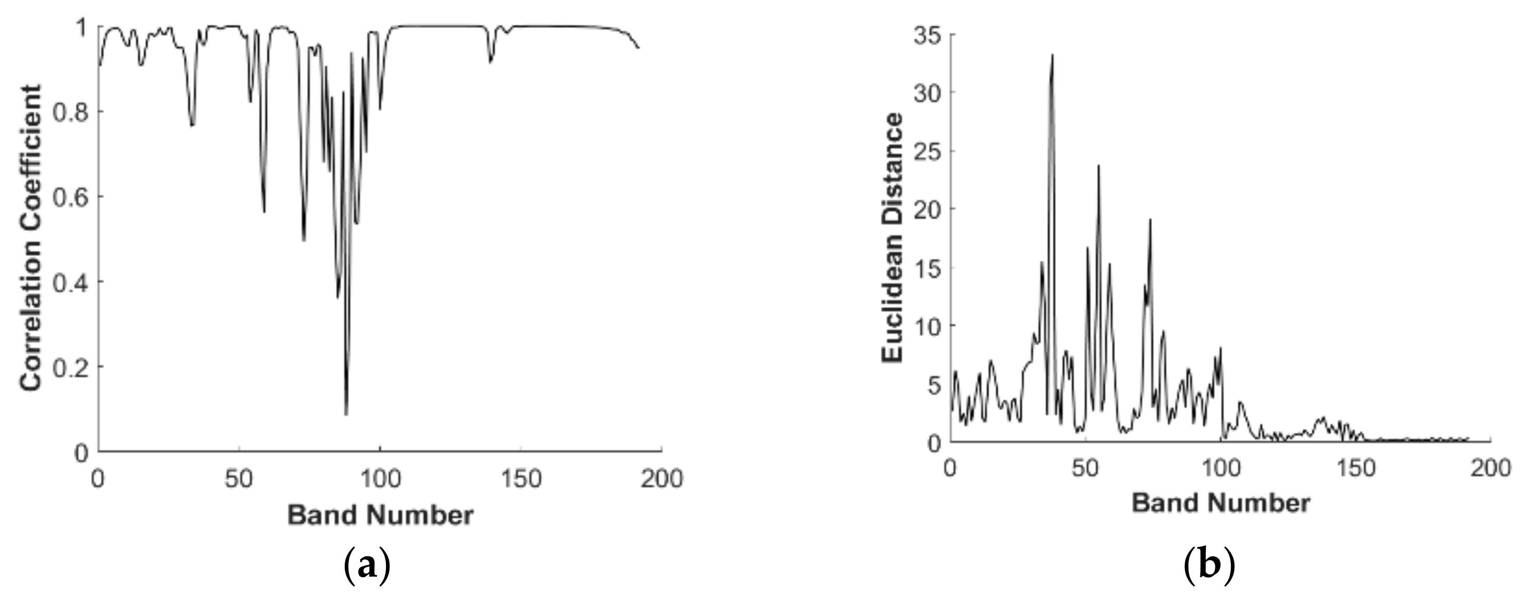
- Calculate the correlation coefficient matrix R of adjacent bands, which is defined as ; or calculate the Euclidean distance matrix D of adjacent bands which is defined as .
- (3)
- The local minimum of correlation coefficient matrix R or the local maximum of the Euclidean distance matrix D is obtained by smoothing the correlation vectors. Suppose the local minimum or maximum is S. If S > M, take the previous M − 1 values as nodes, and divide the hyperspectral data cube into M data subspaces. Otherwise, it can only be divided into S + 1 data subspaces.
2.1.3. Coarse-Fine Partition Method
- (1)
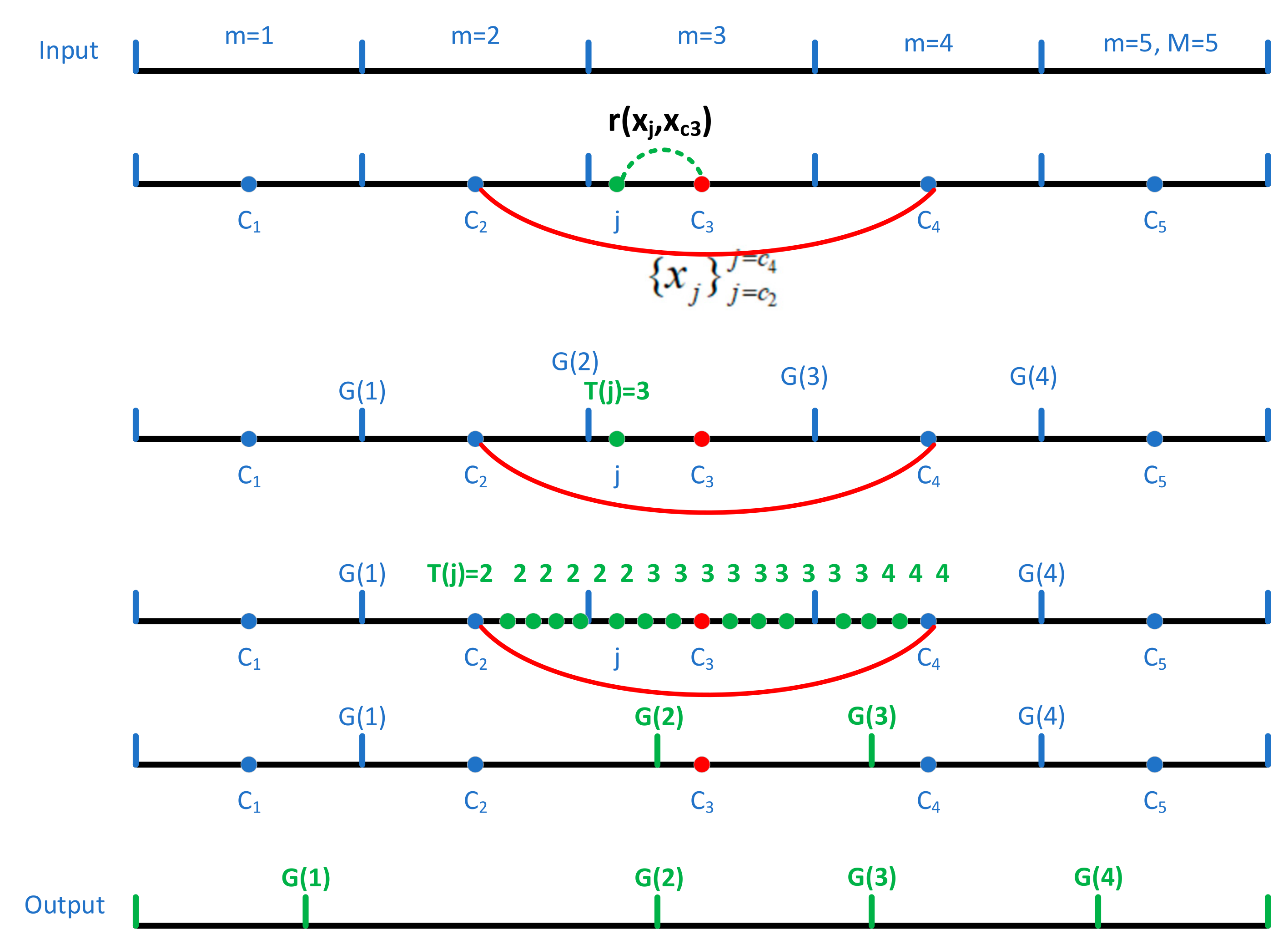
- Define R to record the correlation between the current band and the central band , and initialize R to zero. The subspace label is defined as T which is initialized to zero.
- (2)
- Calculate the correlation coefficient between the current band and the central band . The correlation between the two bands can be regarded as the similarity between them. The greater the correlation, the higher the similarity.
- (3)
- If , set and .
- (4)
- Traverse the neighborhood bands of each central band .
- (5)
- Remove the influence of the noise. The label value obtained by a neighborhood subspace may be [1,1,1,1,1,2,2,2], and the intermediate label value of 2 may be influenced by noise. A singular value should be removed to avoid noise interference.
- (6)
- In subspace m, for the current band , if , T(j) = m − 1; if , T(j) = m + 1; else T(j) = m; for , if T(j − 1) = m, and T(j) = m + 1, the new band partition node of subspace m is G(m), G(m) = j.
- (7)
- Obtain the fine subspace of the hyperspectral data cube .
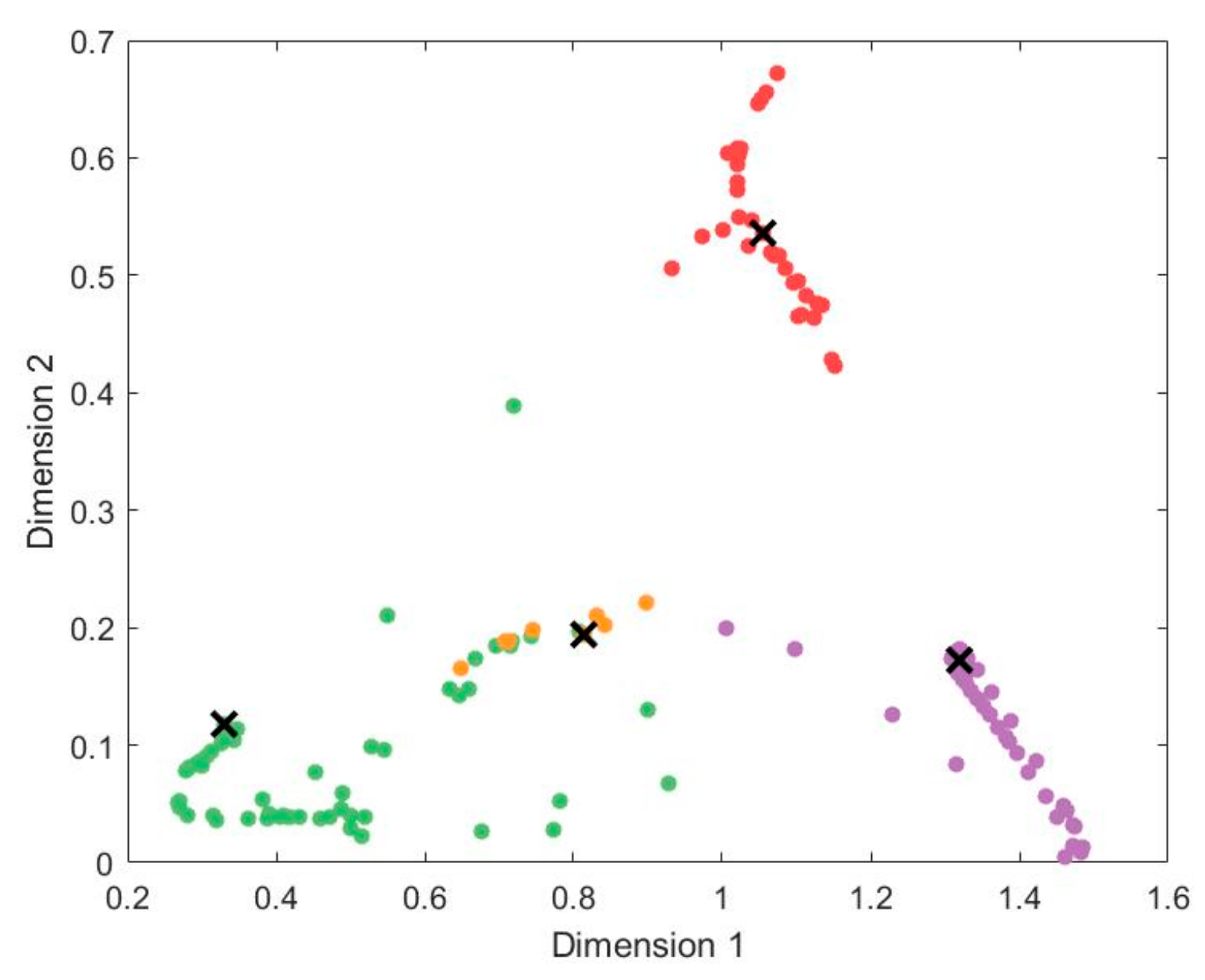
2.1.4. K-Means Method
- (1)
- From L bands, according to the principle of equal-spacing partition, each equal-spacing subset is taken as the initial cluster to find M cluster centers (M = 1,2… M) as the initial clustering center, and the cluster label T is defined.
- (2)
- For two adjacent cluster centers of and , and for each band of , calculate the Euclidean distance and between , and , and between and , and take the label of the cluster center with a smaller Euclidean distance as the updated cluster label of this band.
- (3)
- Recalculate the center of each cluster
- (4)
- Repeat Steps (2) and (3) until all cluster centers do not change or the maximum number of iterations is reached.
- (5)
- The final M clusters are the desired M subspaces.
- (6)
- If the cluster label is not continuous (e.g., the cluster label is... 1,1,1,1,2,2,1,1,1,1,2,2,2,2...), in other words, if there are noise bands, the discontinuous label must be updated to a label that is closer to the cluster. In the preceding example, 2,2 and 1,1,1,1 denote discontinuous labels. The distance between 2,2 and its cluster is 4, and the distance between 1,1,1,1 and its cluster is 2.
2.2. Spatial–Spectral Joint Information
2.2.1. K-Nearest Neighbor of Pixel Points
2.2.2. Spectral Angle Mapping
2.2.3. Information Entropy
2.2.4. Spatial–Spectral Combination Algorithm
2.2.5. Image Classification
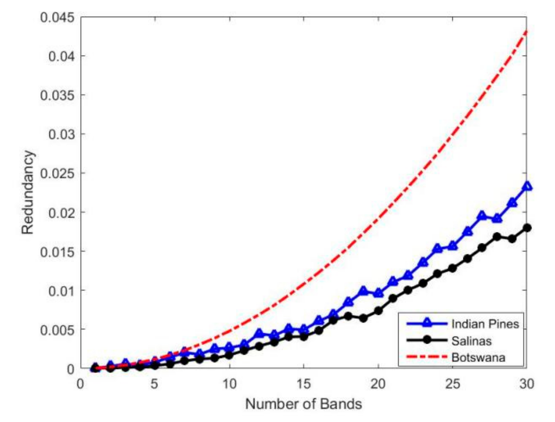
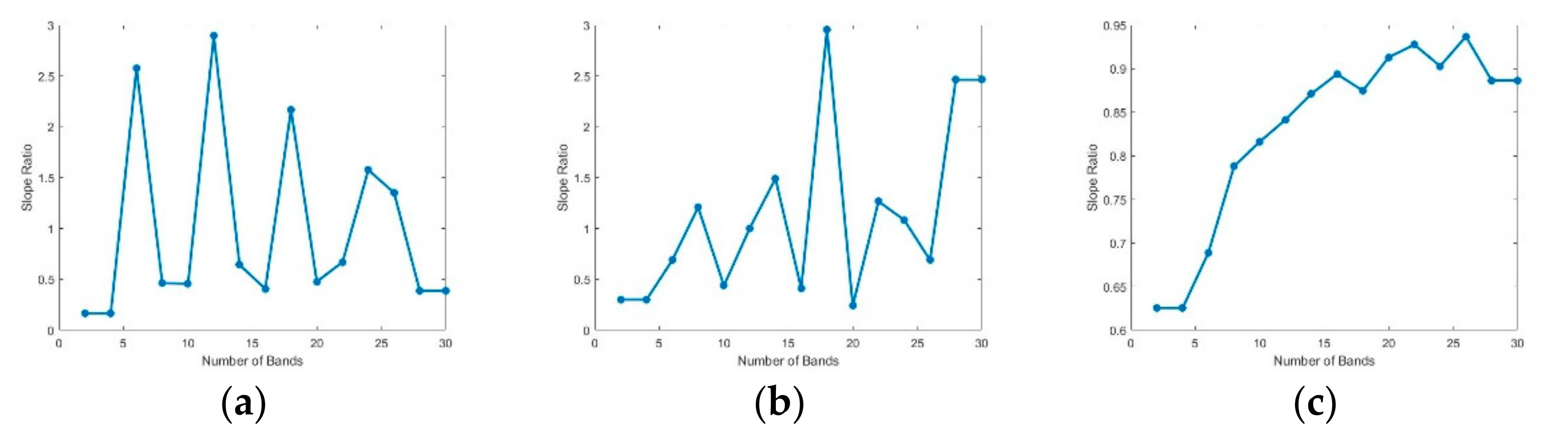
2.2.6. Recommended Number of Bands
3. Experiment
3.1. Data Sets
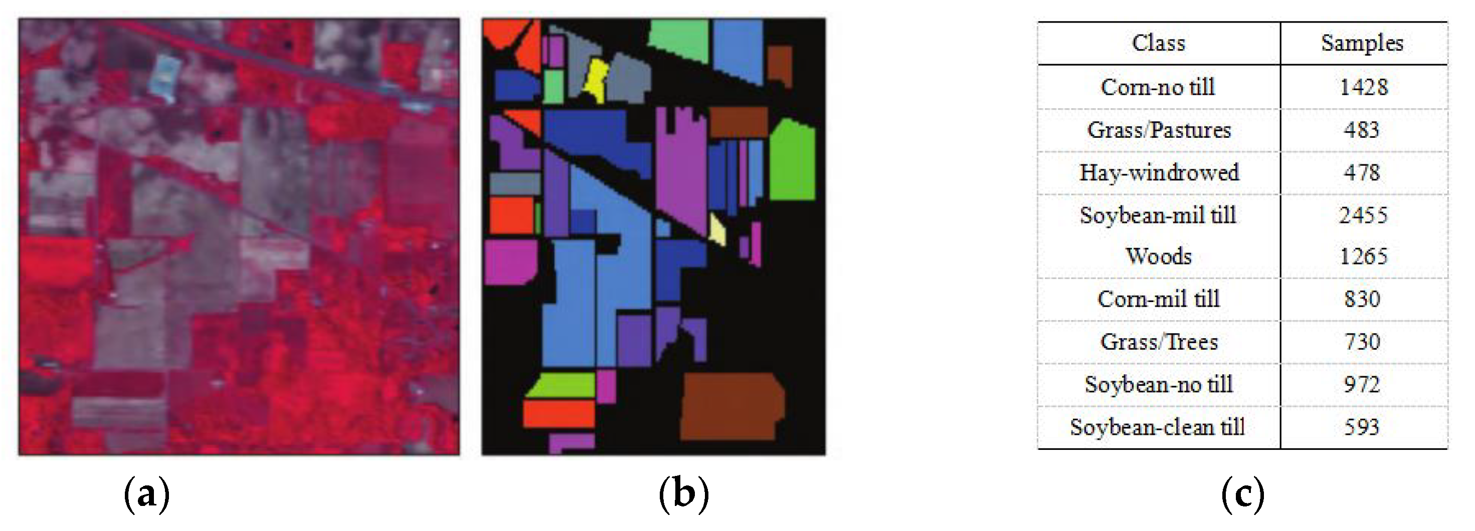
3.1.1. Indian Pines
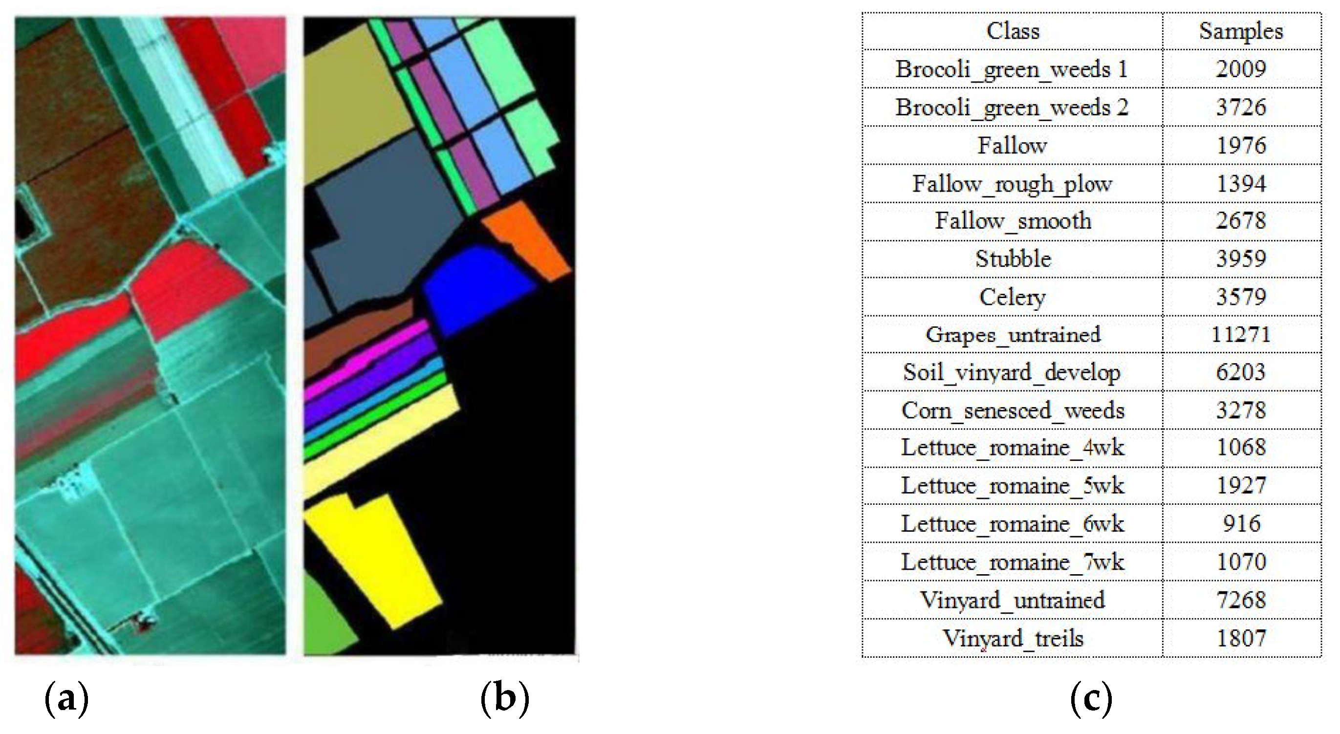
3.1.2. Salinas
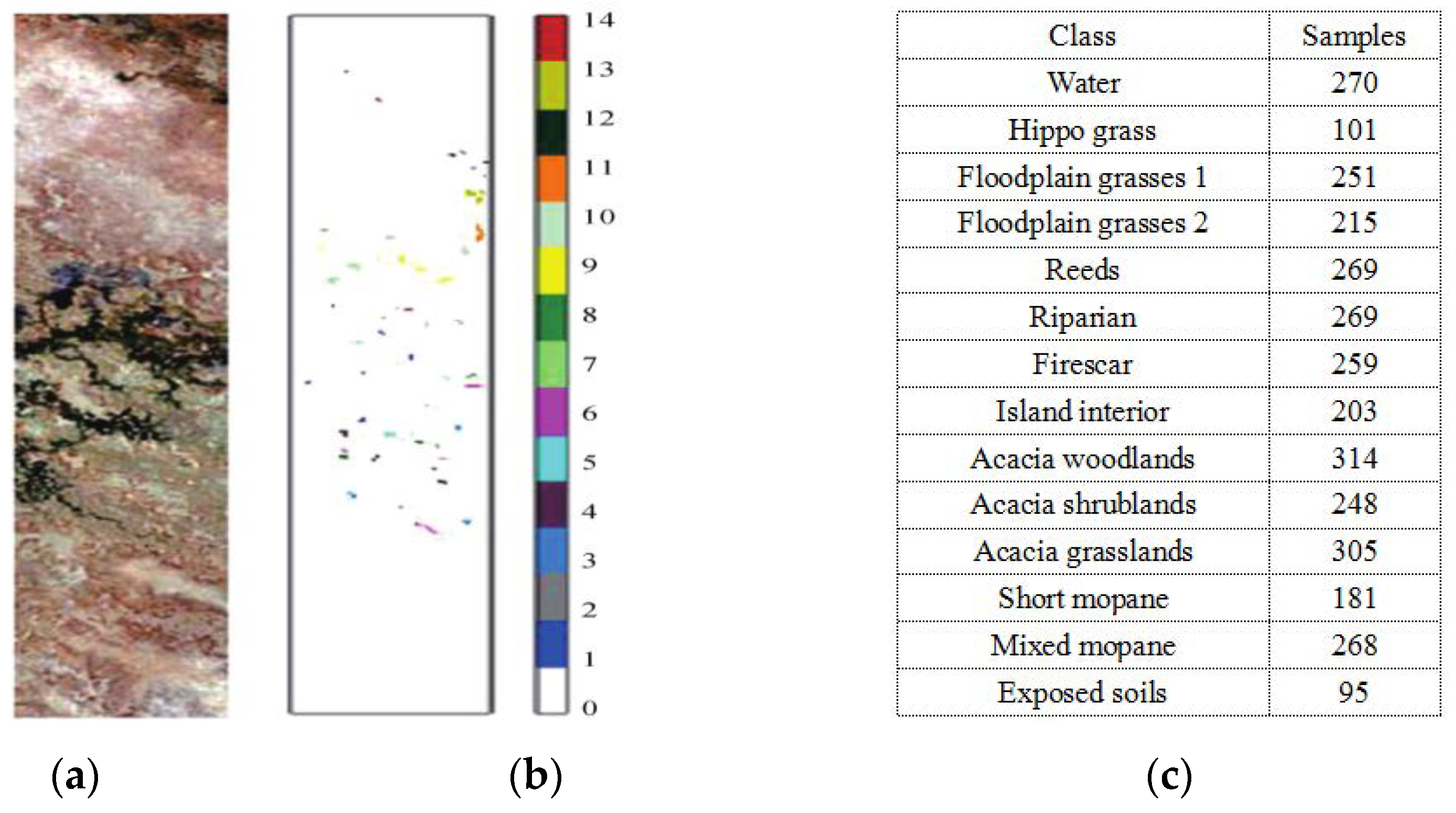
3.1.3. Botswana
3.2. Experimental Setup
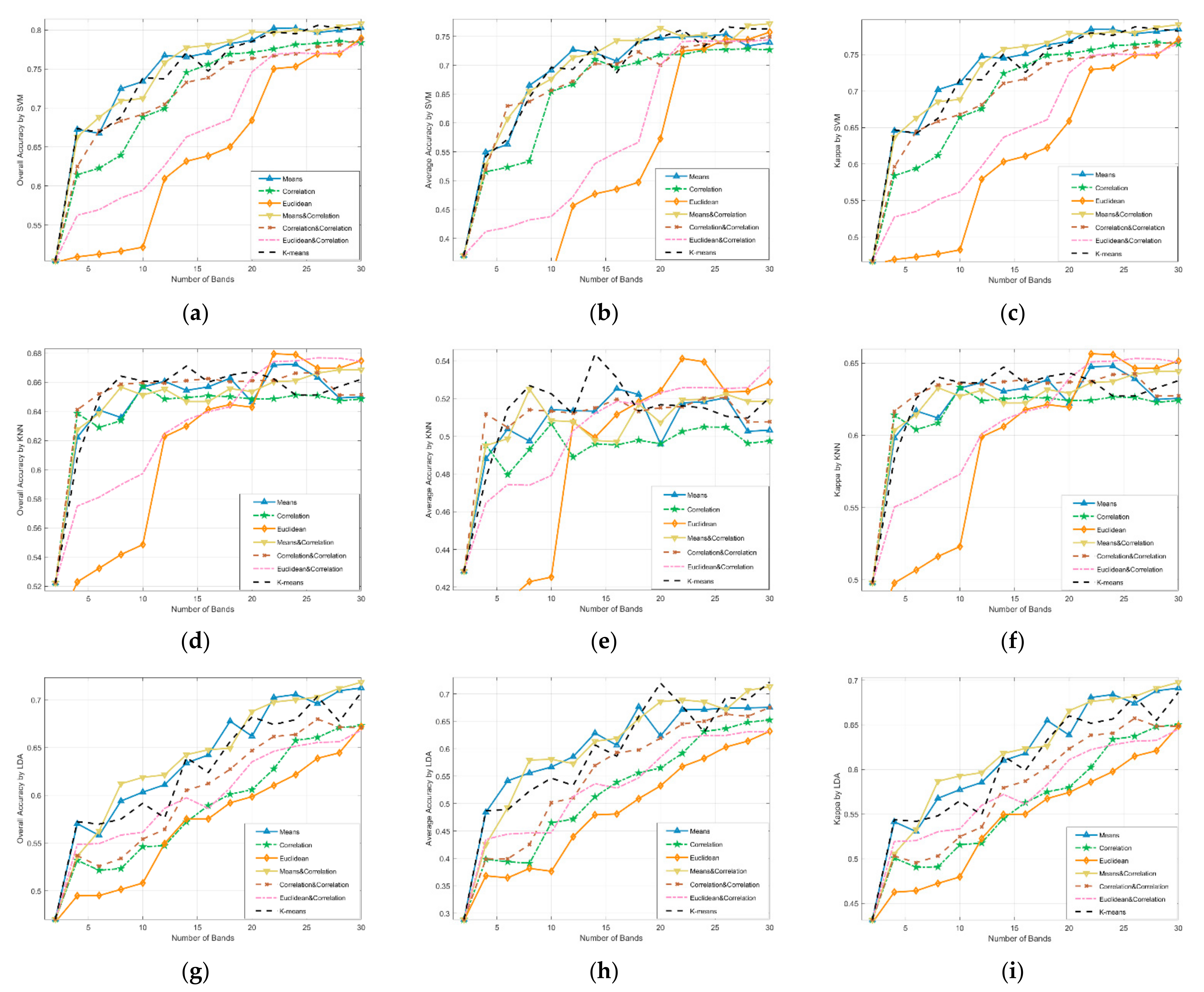
3.3. Comparison of Different Subspace Partitioning Methods
3.4. Experimental Results and Analysis
3.4.1. Recommended Bands
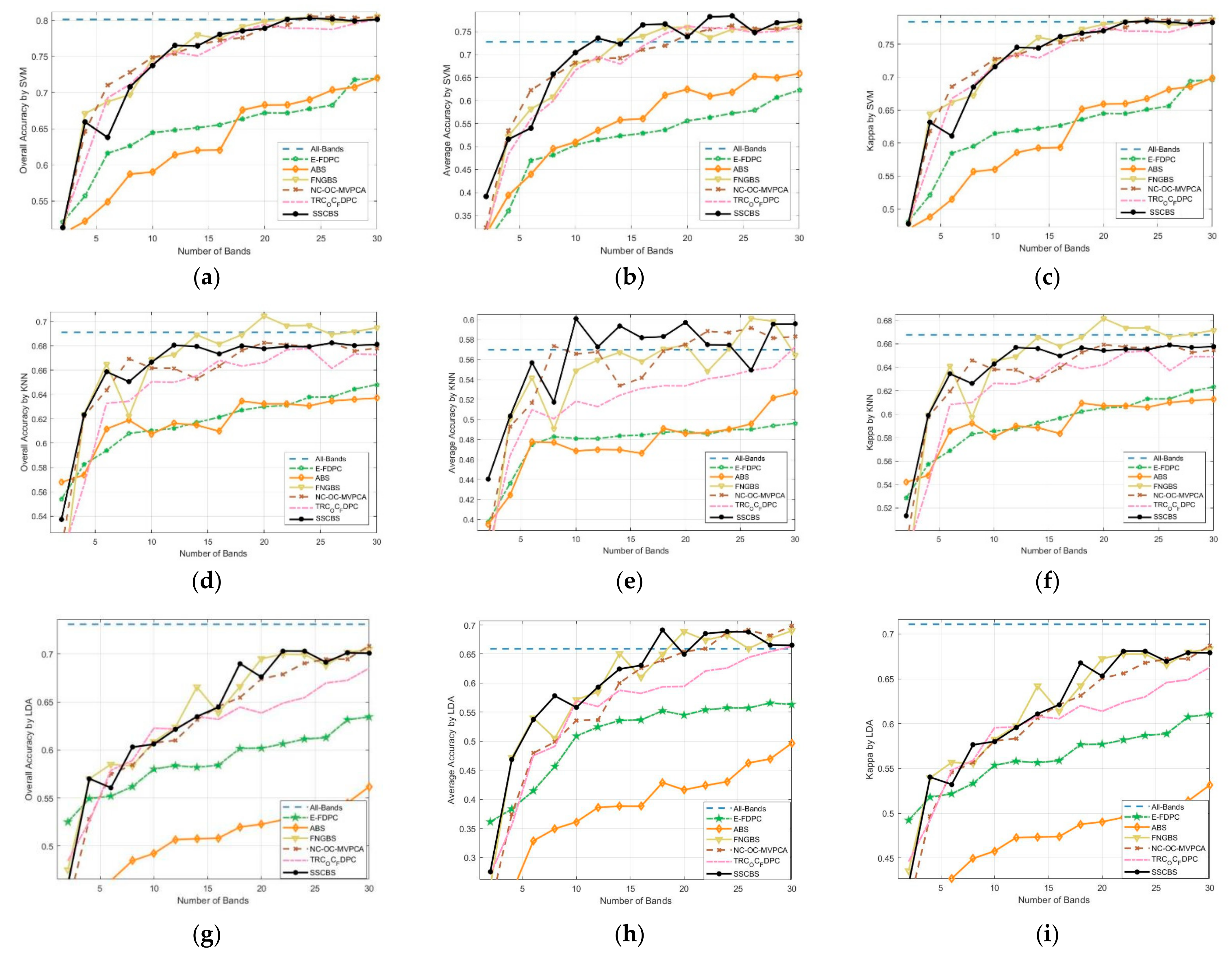
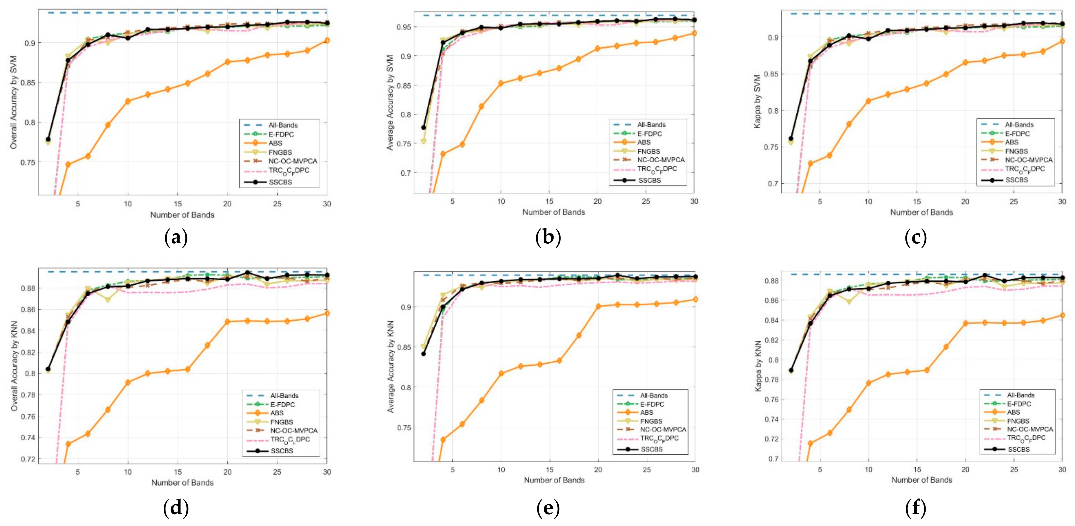
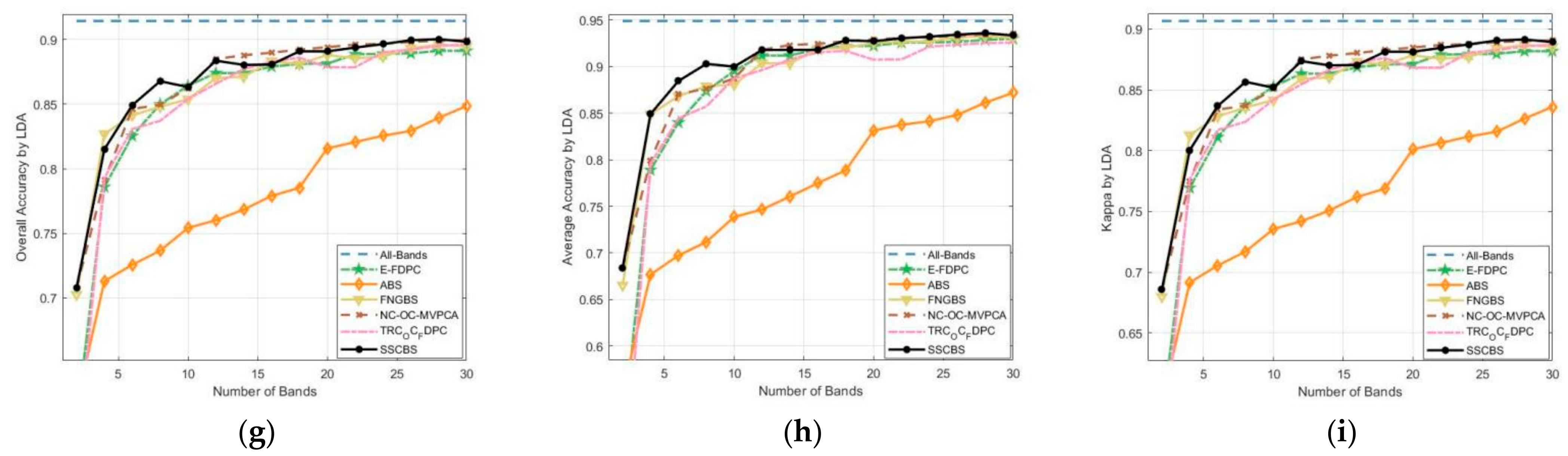
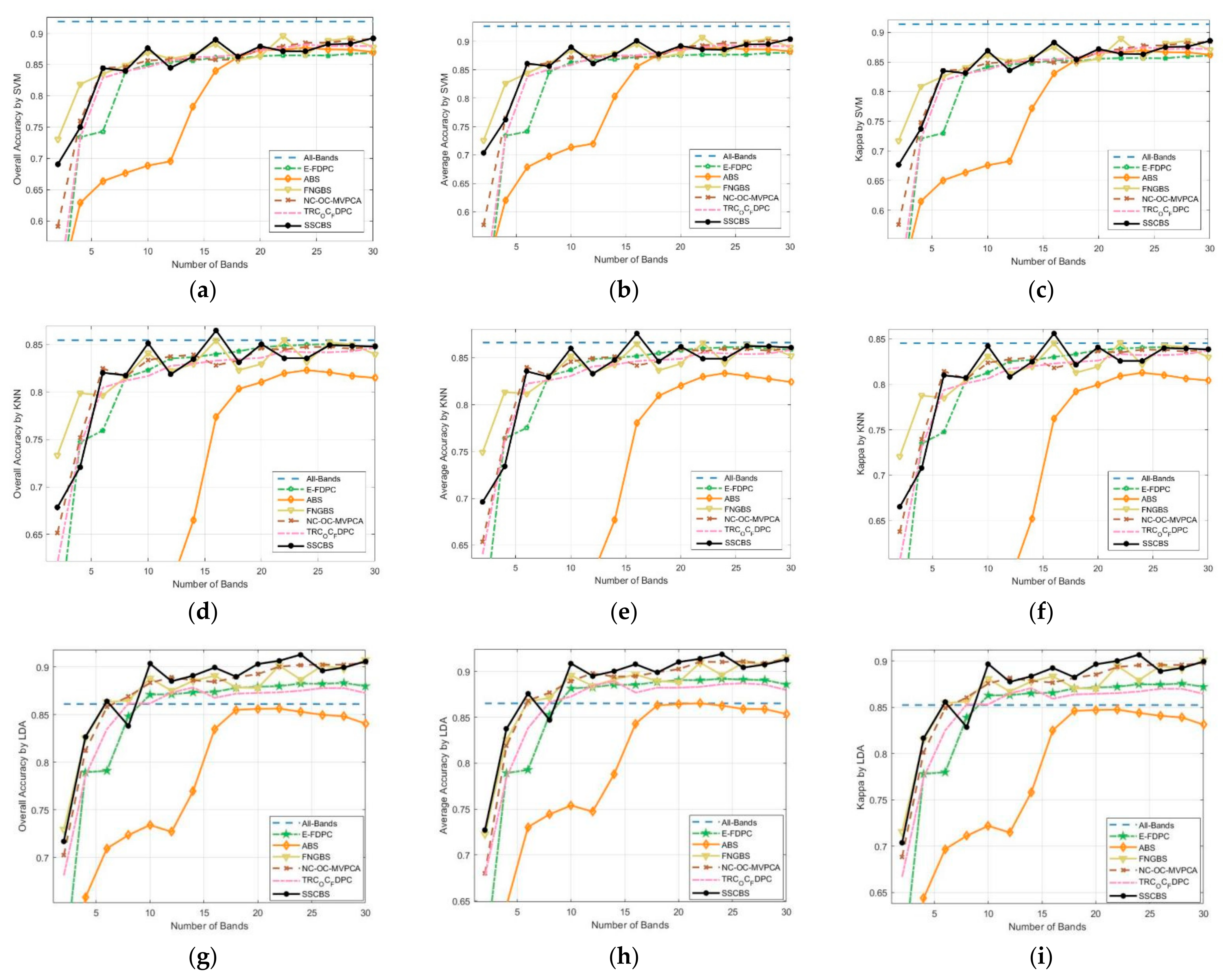
3.4.2. Classification Performance
3.4.3. Computational Time
4. Conclusions
Author Contributions
Funding
Data Availability Statement
Conflicts of Interest
References
- Lishuan, H. Study of Dimensionality Reduction and Spatial-Spectral Method for Classification of Hyperspectral Remote Sensing Image; China University of Geosciences: Wuhan, China, 2018. [Google Scholar]
- Plaza, A.; Benediktsson, J.A.; Boardman, J.W.; Brazile, J.; Bruzzone, L.; Camps-Valls, G.; Chanussot, J.; Fauvel, M.; Gamba, P.; Gualtieri, A.; et al. Recent advances in techniques for hyperspectral image processing. Remote Sens. Environ. 2009, 113, S110–S122. [Google Scholar] [CrossRef]
- Hughes, G.F. On the mean accuracy of statistical pattern recognizers. IEEE Trans. Inf. Theory 1968, IT-14, 55–63. [Google Scholar] [CrossRef] [Green Version]
- Guo, B.; Gunn, S.R.; Damper, R.I.; Nelson, J.D.B. Band selection for hyperspectral image classification using mutual information. IEEE Geosci. Remote Sens. Lett. 2006, 3, 522–526. [Google Scholar] [CrossRef] [Green Version]
- Sun, W.; Halevy, A.; Benedetto, J.J.; Czaja, W.; Li, W.; Liu, C.; Shi, B.; Wang, R. Nonlinear dimensionality reduction via the ENHLTSA method for hyperspectral image classification. IEEE J. Sel. Topics Appl. Earth Observ. Remote Sens. 2014, 7, 375–388. [Google Scholar] [CrossRef]
- Lu, T.; Li, S.; Fang, L.; Ma, Y.; Benediktsson, J.A. Spectral–spatial adaptive sparse representation for hyperspectral image denoising. IEEE Trans. Geosci. Remote Sens. 2016, 54, 373–385. [Google Scholar] [CrossRef]
- Geng, X.; Sun, K.; Ji, L.; Zhao, Y. A fast volume-gradient-based band selection method for hyperspectral image. IEEE Trans. Geosci. Remote Sens. 2014, 52, 7111–7119. [Google Scholar] [CrossRef]
- Luis, O.J.; David, A.L. Hyperspectral data analysis and supervised feature reduction via projection pursuit. IEEE Trans. Geosci. Remote Sens. 1999, 37, 2653–2667. [Google Scholar]
- Jia, X.; Richards, J.A. Segmented principal components transformation for efficient hyperspectral remote sensing image display and classification. IEEE Trans. Geosci. Remote Sens. 1999, 37, 538–542. [Google Scholar]
- He, X.; Niyogi, P. Locality preserving projections. Proc. Adv. Neural Inf. Process. Syst. 2004, 16, 153–160. [Google Scholar]
- He, X.; Cai, D.; Yan, S.; Zhang, H. Neighborhood preserving embedding. In Proceedings of the 10th IEEE International Conference on Computer Vision, Beijing, China, 17–21 October 2005; Volume 2, pp. 1208–1213. [Google Scholar]
- Friedman, J. Regularized discriminant analysis. J. Am. Stat. Assoc. 1989, 84, 165–175. [Google Scholar] [CrossRef]
- Bandos, T.V.; Bruzzone, L.; Camps-Valls, G. Classification of hyperspectral images with regularized linear discriminant analysis. IEEE Trans. Geosci. Remote Sens. 2009, 47, 862–873. [Google Scholar] [CrossRef]
- Kuo, B.C.; Landgrebe, D.A. Nonparametric weighted feature extraction for classification. IEEE Trans. Geosci. Remote Sens. 2004, 42, 1096–1105. [Google Scholar]
- Sugiyama, M. Dimensionality reduction of multimodal labeled data by localFisher discriminant analysis. J. Mach. Learn. Res. 2007, 8, 1027–1061. [Google Scholar]
- Chen, H.T.; Chang, H.W.; Liu, T.L. Local discriminant embedding and its variants. In Proceedings of the 2005 IEEE Computer Society Conference on Computer Vision and Pattern Recognition (CVPR’05), San Diego, CA, USA, 20–25 June 2005; pp. 846–853. [Google Scholar]
- Yan, S.; Xu, D.; Zhang, B.; Zhang, H.J.; Yang, Q.; Lin, S. Graph embedding and extensions: A general framework for dimensionality reduction. IEEE Trans. Pattern Anal. Mach. Intell. 2007, 29, 40–51. [Google Scholar] [CrossRef] [PubMed] [Green Version]
- Serpico, S.B.; Bruzzone, L. A new search algorithm for feature selection in hyperspectral remote sensing images. IEEE Trans. Geosci. Remote Sens. 2001, 39, 1360–1367. [Google Scholar] [CrossRef]
- Guyon, I.; Elisseeff, A. An introduction to variable and feature selection. J. Mach. Learn. Res. 2003, 3, 1157–1182. [Google Scholar]
- Li, Q.; Wang, Q.; Li, X. An efficient clustering method for hyper- spectral optimal band selection via shared nearest neighbor. Remote Sens. 2019, 11, 350. [Google Scholar] [CrossRef] [Green Version]
- Wang, Q.; Li, Q.; Li, X. Hyperspectral band selection via adaptive subspace partition strategy. IEEE J. Sel. Topics Appl. Earth Observ. Remote Sens. 2019, 12, 4940–4950. [Google Scholar] [CrossRef]
- Yang, H.; Du, Q.; Su, H.; Sheng, Y. An efficient method for supervised hyperspectral band selection. IEEE Geosci. Remote Sens. Lett. 2011, 8, 138–142. [Google Scholar] [CrossRef]
- Archibald, R.; Fann, G. Feature selection and classification of hyperspectral images with support vector machines. IEEE Geosci. Remote Sens. Lett. 2007, 4, 674–677. [Google Scholar] [CrossRef]
- Bai, J.; Xiang, S.; Pan, C. Classification oriented semi-supervised band selection for hyperspectral images. In Proceedings of the 21st International Conference on Pattern Recognition, Tsukuba, Japan, 11–15 November 2012; pp. 1888–1891. [Google Scholar]
- Chen, L.; Huang, R.; Huan, W. Graph-based semi-supervised weighted band selection for classification of hyperspectral data. In Proceedings of the 2010 International Conference on Audio, Language and Image Processing, Shanghai, China, 23–25 November 2010; pp. 1123–1126. [Google Scholar]
- Reza, M.; Ghamary, M.; Mojaradi, B. Unsupervised feature selection using geometrical measures in prototype space for hyperspectral imagery. IEEE Trans. Geosci. Remote Sens. 2014, 52, 3774–3787. [Google Scholar]
- Chunhong, L.; Chunhui, Z.; Lingyan, Z. A new dimensionality reduction method for hyperspectral remote sensing image. J. Image Graph. 2005, 10, 218–223. [Google Scholar]
- Jia, S.; Tang, G.; Zhu, J.; Li, Q. A Novel Ranking-Based Clustering Approach for Hyperspectral Band Selection. IEEE Trans. Geosci. Remote Sens. 2016, 54, 88–102. [Google Scholar] [CrossRef]
- Qi, W.; Qiang, L.; Xuelong, L. A Fast Neighborhood Grouping Method for Hyperspectral Band Selection. IEEE Trans. Geosci. Remote Sens. 2021, 59, 5028–5039. [Google Scholar]
- Wang, Q.; Zhang, F.H.; Li, X.L. Optimal clustering framework for hyperspectral band selection. IEEE Trans. Geosci. Remote Sens. 2018, 56, 5910–5922. [Google Scholar] [CrossRef] [Green Version]
- Zhou, Y.; Peng, J.; Chen, C. Dimension Reduction Using Spatial and Spectral Regularized Local Discriminant Embedding for Hyperspectral Image Classification. IEEE Trans. Geosci. Remote Sens. 2015, 53, 1082–1095. [Google Scholar] [CrossRef]
- Huang, H.; Shi, G.; He, H.; Duan, Y.; Luo, F. Dimensionality Reduction of Hyperspectral Imagery Based on Spatial-spectral Manifold Learning. arXiv 2018, arXiv:1812.09530. [Google Scholar] [CrossRef] [Green Version]
- Zhou, L.; Zhang, X. Discriminative spatial-spectral manifold embedding for hyperspectral image classification. Remote Sens. Lett. 2015, 6, 715–724. [Google Scholar] [CrossRef]
- Zhao, W.; Du, S. Spectral–Spatial Feature Extraction for Hyperspectral Image Classification: A Dimension Reduction and Deep Learning Approach. IEEE Trans. Geosci. Remote Sens. 2016, 54, 4544–4554. [Google Scholar] [CrossRef]
- Feng, Z.; Yang, S.; Wang, S.; Jiao, L. Discriminative Spectral–Spatial Margin-Based Semi-supervised Dimensionality Reduction of Hyperspectral Data. IEEE Geosci. Remote Sens. Lett. 2015, 12, 224–228. [Google Scholar] [CrossRef]
- Bai, X.; Guo, Z.; Wang, Y.; Zhang, Z.; Zhou, J. Semi-supervised Hyperspectral Band Selection Via Spectral–Spatial Hypergraph Model. IEEE J. Sel. Top. Appl. Earth Obs. Remote Sens. 2015, 8, 2774–2783. [Google Scholar] [CrossRef] [Green Version]
- Liang, Z.; Liguo, W.; Danfeng, L. A subspace band selection method for hyperspectral imagery. J. Remote Sens. 2019, 23, 904–910. [Google Scholar]
- Dehui, Z.; Bo, D.; Liangpei, Z. Band selection-based collaborative representation for anomaly detection in hyperspectral images. J. Remote Sens. 2020, 24, 427–438. [Google Scholar]
- Yanlong, C.; Xiaolan, W.; En, L.; Mei-ping, S.; Hai-mo, B. Research and Application of Band Selection Method Based on CEM. Spectrosc. Spectr. Anal. 2020, 40, 3778–3783. [Google Scholar]
- Fuquan, Z.; Huajun, W.; Liping, Y.; Changguo, L. Hyperspectral image lossless compression using adaptive bands selection and optimal prediction sequence. Opt. Precis. Eng. 2020, 28, 1609–1617. [Google Scholar]
- Pal, M.; Foody, G.M. Feature selection for classification of hyperspectral data by SVM. IEEE Trans. Geosci. Remote Sens. 2010, 48, 2297–2307. [Google Scholar] [CrossRef] [Green Version]
- Kulesza, A. Determinantal point processes for machine learning. Found. Trends Mach. Learn. 2012, 5, 123–286. [Google Scholar] [CrossRef]


| Classifier | Classification Accuracy | Means | Correlation | Euclidean | Means and Correlation | Correlation and Correlation | Euclidean and Correlation | K-Means |
|---|---|---|---|---|---|---|---|---|
| SVM | OA | 0.7447 ± 0.0134 | 0.7083 ± 0.0182 | 0.6371 ± 0.0203 | 0.7430 ± 0.0149 | 0.7182 ± 0.0097 | 0.6668 ± 0.0231 | 0.7398 ± 0.0189 |
| AA | 0.6752 ± 0.0207 | 0.6333 ± 0.0156 | 0.5171 ± 0.0279 | 0.6872 ± 0.0156 | 0.6675 ± 0.0221 | 0.5613 ± 0.0173 | 0.6747 ± 0.0129 | |
| Kappa | 0.7230 ± 0.0245 | 0.6847 ± 0.0203 | 0.6078 ± 0.0168 | 0.7212 ± 0.0218 | 0.6950 ± 0.0147 | 0.6398 ± 0.0263 | 0.7177 ± 0.0136 | |
| t(s) | 0.0001 ± 2E-5 | 0.0519 ± 0.0042 | 0.0296 ± 0.0022 | 9.7414 ± 0.068 | 9.9139 ± 0.093 | 9.9949 ± 0.075 | 9.8488 ± 0.084 | |
| KNN | OA | 0.6506 ± 0.0276 | 0.6442 ± 0.0159 | 0.6089 ± 0.0145 | 0.6475 ± 0.0224 | 0.6497 ± 0.0178 | 0.6263 ± 0.0126 | 0.6524 ± 0.0214 |
| AA | 0.5172 ± 0.0157 | 0.5069 ± 0.0166 | 0.4898 ± 0.0275 | 0.5152 ± 0.0243 | 0.5144 ± 0.0176 | 0.5110 ± 0.0189 | 0.5154 ± 0.0177 | |
| Kappa | 0.6271 ± 0.0173 | 0.6202 ± 0.0211 | 0.5852 ± 0.0156 | 0.6240 ± 0.0264 | 0.6262 ± 0.0166 | 0.6030 ± 0.0197 | 0.6289 ± 0.0208 | |
| t(s) | 0.0001 ± 3E-5 | 0.0536 ± 0.0025 | 0.0295 ± 0.0032 | 10.1750 ± 0.068 | 10.3461 ± 0.088 | 10.3837 ± 0.093 | 10.1713 ± 0.079 | |
| LDA | OA | 0.6364 ± 0.0187 | 0.5829 ± 0.0245 | 0.5734 ± 0.0166 | 0.6396 ± 0.0204 | 0.5989 ± 0.0198 | 0.6043 ± 0.0231 | 0.6307 ± 0.0187 |
| AA | 0.6134 ± 0.0239 | 0.5204 ± 0.0223 | 0.4889 ± 0.0169 | 0.6061 ± 0.0251 | 0.5468 ± 0.0297 | 0.5345 ± 0.0307 | 0.6040 ± 0.0163 | |
| Kappa | 0.6115 ± 0.0218 | 0.5546 ± 0.0266 | 0.5463 ± 0.0285 | 0.6146 ± 0.0223 | 0.5710 ± 0.0153 | 0.5783 ± 0.0286 | 0.6055 ± 0.0266 | |
| t(s) | 0.0001 ± 2E-5 | 0.0447 ± 0.0039 | 0.0267 ± 0.0080 | 7.6649 ± 0.089 | 7.8705 ± 0.069 | 7.8880 ± 0.082 | 7.6763 ± 0.057 |
| Dataset | Classifier | Method | ||||||
|---|---|---|---|---|---|---|---|---|
| M | E-FDPC | ABS | FNGBS | NC_OC_MVPCA | TRC_OC_FDPC | SSCBS | ||
| Indian Pines | 6 | SVM | 0.4693 ± 0.0218 | 0.4392 ± 0.0196 | 0.5816 ±0.0309 | 0.6224 ± 0.0383 | 0.5598 ± 0.0276 | 0.5397 ± 0.0223 |
| KNN | 0.475 ± 0.0133 | 0.4778 ± 0.0088 | 0.5417 ±0.0332 | 0.5168 ± 0.0315 | 0.5098 ± 0.0235 | 0.5568 ± 0.0187 | ||
| LDA | 0.4515 ± 0.0143 | 0.3274 ± 0.0093 | 0.5281 ±0.0328 | 0.4707 ± 0.0421 | 0.4743 ± 0.0274 | 0.5276 ± 0.0258 | ||
| 12 | SVM | 0.5147 ± 0.0147 | 0.5348 ± 0.0120 | 0.6895 ± 0.0356 | 0.692 ± 0.0302 | 0.6944 ± 0.0286 | 0.7354 ± 0.0278 | |
| KNN | 0.481 ± 0.0279 | 0.47 ± 0.0056 | 0.5596 ± 0.0259 | 0.5677 ± 0.0409 | 0.5129 ± 0.0210 | 0.5726 ± 0.0381 | ||
| LDA | 0.5562 ± 0.0304 | 0.3938 ± 0.0027 | 0.5984 ± 0.0251 | 0.5513 ± 0.0358 | 0.5674 ± 0.0246 | 0.5792 ± 0.0295 | ||
| 18 | SVM | 0.536 ± 0.0215 | 0.6117 ± 0.0084 | 0.7587 ± 0.0195 | 0.7193 ± 0.0295 | 0.7454 ± 0.0247 | 0.7663 ± 0.0216 | |
| KNN | 0.4872 ± 0.0294 | 0.4912 ± 0.0078 | 0.5705 ± 0.0155 | 0.5686 ± 0.0406 | 0.5338 ± 0.0224 | 0.5829 ± 0.0224 | ||
| LDA | 0.5532 ± 0.0217 | 0.444 ± 0.0108 | 0.6368 ± 0.0292 | 0.634 ± 0.0327 | 0.5935 ± 0.0268 | 0.6553 ± 0.0218 | ||
| 24 | SVM | 0.5722 ± 0.0210 | 0.6181 ± 0.0125 | 0.7546 ± 0.0357 | 0.7628 ± 0.0269 | 0.7566 ± 0.0394 | 0.7836 ± 0.0169 | |
| KNN | 0.4899 ± 0.0341 | 0.4903 ± 0.0102 | 0.571 ± 0.0014 | 0.587 ± 0.0287 | 0.5439 ± 0.0281 | 0.5745 ± 0.0052 | ||
| LDA | 0.5558 ± 0.0157 | 0.439 ± 0.0047 | 0.6515 ± 0.0368 | 0.7032 ± 0.0294 | 0.6338 ±0.0357 | 0.6847 ± 0.0259 | ||
| 30 | SVM | 0.6227 ± 0.0157 | 0.6586 ± 0.0102 | 0.7675 ± 0.027 | 0.7583 ± 0.0237 | 0.7598 ± 0.0248 | 0.7728 ± 0.0213 | |
| KNN | 0.4963 ± 0.0425 | 0.5271 ± 0.0317 | 0.5645 ± 0.0073 | 0.5831 ± 0.0261 | 0.5727 ± 0.0413 | 0.5957 ± 0.0187 | ||
| LDA | 0.5662 ± 0.0158 | 0.4993 ± 0.0196 | 0.6819 ± 0.0286 | 0.72 ± 0.0302 | 0.6528 ± 0.0267 | 0.6672 ± 0.0158 | ||
| Salians | 6 | SVM | 0.9388 ± 0.0157 | 0.7484 ± 0.0014 | 0.9399 ± 0.0119 | 0.9428 ± 0.0135 | 0.9321 ± 0.0237 | 0.94 ± 0.0153 |
| KNN | 0.9237 ± 0.0132 | 0.7542 ± 0.0125 | 0.9257 ± 0.0147 | 0.9267 ± 0.0204 | 0.9215 ± 0.0138 | 0.9218 ± 0.0149 | ||
| LDA | 0.8415 ± 0.0179 | 0.6984 ± 0.0093 | 0.8684 ± 0.0148 | 0.8741 ± 0.0151 | 0.8437 ± 0.0197 | 0.8863 ± 0.0104 | ||
| 12 | SVM | 0.9501 ± 0.0178 | 0.8618 ± 0.0156 | 0.9527 ± 0.0147 | 0.9537 ± 0.0249 | 0.9529 ± 0.0193 | 0.9545 ± 0.0172 | |
| KNN | 0.9328 ± 0.0138 | 0.8262 ± 0.0094 | 0.932 ± 0.0273 | 0.9308 ± 0.0192 | 0.9263 ± 0.0124 | 0.9339 ± 0.0204 | ||
| LDA | 0.9128 ± 0.0084 | 0.7474 ± 0.0047 | 0.905 ± 0.0138 | 0.918 ± 0.0216 | 0.8973 ± 0.0273 | 0.9178 ± 0.0178 | ||
| 18 | SVM | 0.958 ± 0.0197 | 0.8945 ± 0.0117 | 0.9538 ± 0.0180 | 0.958 ± 0.0132 | 0.9572 ± 0.0208 | 0.9574 ± 0.0153 | |
| KNN | 0.9371 ± 0.0196 | 0.8644 ±0.0148 | 0.9322 ± 0.0284 | 0.9327 ± 0.0235 | 0.929 ± 0.0148 | 0.9349 ± 0.0150 | ||
| LDA | 0.9236 ± 0.0146 | 0.7875 ± 0.0153 | 0.9198 ± 0.0186 | 0.9269 ± 0.0138 | 0.9178 ± 0.0196 | 0.9292 ± 0.0153 | ||
| 24 | SVM | 0.9591 ± 0.0205 | 0.9224 ± 0.0174 | 0.9569 ± 0.0208 | 0.961 ± 0.0156 | 0.9603 ± 0.0195 | 0.9593 ± 0.0147 | |
| KNN | 0.9337 ± 0.0140 | 0.9027 ± 0.0196 | 0.9312 ± 0.0146 | 0.9348 ± 0.0207 | 0.9296 ± 0.0147 | 0.9352 ± 0.0084 | ||
| LDA | 0.9266 ± 0.0168 | 0.8409 ± 0.0147 | 0.9257 ± 0.0185 | 0.932 ± 0.0296 | 0.9229 ± 0.0157 | 0.9306 ± 0.0161 | ||
| 30 | SVM | 0.9603 ± 0.0159 | 0.939 ± 0.0102 | 0.9618 ± 0.0162 | 0.963 ± 0.0147 | 0.9626 ± 0.0205 | 0.9616 ± 0.0159 | |
| KNN | 0.9351 ± 0.0149 | 0.9092 ± 0.0175 | 0.9342 ± 0.0256 | 0.9357 ± 0.0196 | 0.9316 ± 0.0135 | 0.9377 ± 0.0115 | ||
| LDA | 0.9301 ± 0.0154 | 0.8748 ± 0.0102 | 0.9298 ± 0.0157 | 0.9346 ± 0.0179 | 0.9274 ± 0.0271 | 0.9328 ± 0.0143 | ||
| Botswana | 6 | SVM | 0.7413 ± 0.0234 | 0.6787 ± 0.0157 | 0.8439 ± 0.0275 | 0.8587 ± 0.0235 | 0.8379 ± 0.0186 | 0.861 ± 0.0169 |
| KNN | 0.7752 ± 0.0157 | 0.6319 ± 0.0177 | 0.8115 ± 0.0286 | 0.8399 ± 0.0223 | 0.8223 ± 0.0288 | 0.8355 ± 0.0213 | ||
| LDA | 0.818 ± 0.0286 | 0.7339 ± 0.0254 | 0.8821 ± 0.0271 | 0.8734 ± 0.0209 | 0.8642 ± 0.0374 | 0.8763 ± 0.0196 | ||
| 12 | SVM | 0.8671 ± 0.0237 | 0.7199 ± 0.0211 | 0.8732 ± 0.0297 | 0.873 ± 0.0317 | 0.8711 ± 0.0211 | 0.861 ± 0.0169 | |
| KNN | 0.8485 ± 0.0260 | 0.6188 ± 0.0182 | 0.8335 ± 0.0299 | 0.8497 ± 0.0301 | 0.8408 ± 0.0223 | 0.8329 ± 0.0297 | ||
| LDA | 0.8894 ± 0.0280 | 0.7514 ± 0.0214 | 0.9002 ± 0.0166 | 0.8951 ± 0.0183 | 0.8868 ± 0.0288 | 0.8876 ± 0.0209 | ||
| 18 | SVM | 0.8714 ± 0.0281 | 0.8763 ± 0.0197 | 0.8712 ± 0.0212 | 0.8732 ± 0.0231 | 0.8797 ± 0.0375 | 0.8777 ± 0.0280 | |
| KNN | 0.8548 ± 0.0297 | 0.8094 ± 0.0275 | 0.8365 ± 0.0269 | 0.8463 ± 0.0234 | 0.8478 ± 0.0127 | 0.8464 ± 0.0251 | ||
| LDA | 0.8938 ± 0.0286 | 0.8588 ± 0.0163 | 0.8964 ± 0.0218 | 0.8973 ± 0.0264 | 0.8922 ± 0.0188 | 0.9001 ± 0.0157 | ||
| 24 | SVM | 0.8764 ± 0.0175 | 0.8885 ± 0.0191 | 0.8798 ± 0.0144 | 0.897 ± 0.0219 | 0.8937 ± 0.0157 | 0.8853 ± 0.0136 | |
| KNN | 0.861 ± 0.0188 | 0.8336 ± 0.0098 | 0.8441 ± 0.0127 | 0.8596 ± 0.0274 | 0.8546 ± 0.0146 | 0.849 ± 0.0124 | ||
| LDA | 0.8945 ± 0.0286 | 0.8624 ± 0.0189 | 0.8973 ± 0.0145 | 0.9082 ± 0.0269 | 0.8922 ± 0.0128 | 0.9066 ± 0.0087 | ||
| 30 | SVM | 0.8801 ± 0.0143 | 0.8824 ± 0.0186 | 0.8897 ± 0.0162 | 0.9025 ± 0.0121 | 0.8911 ± 0.0198 | 0.9041 ± 0.0087 | |
| KNN | 0.8589 ± 0.0175 | 0.8241 ± 0.0188 | 0.8522 ± 0.0223 | 0.8607 ± 0.0129 | 0.8584 ± 0.0186 | 0.861 ± 0.0213 | ||
| LDA | 0.8945 ± 0.0166 | 0.8594 ± 0.0159 | 0.9022 ± 0.0035 | 0.9067 ± 0.0068 | 0.8906 ± 0.0082 | 0.9068 ± 0.0034 | ||
| Data set | Classifier | E-FDPC | ABS | FNGBS | NC_OC_MVPCA | TRC_OC_FDPC | SSCBS |
|---|---|---|---|---|---|---|---|
| Indian Pines | SVM | 0.0948 | 0.5413 | 0.4326 | 0.6399 | 0.7779 | 0.3918 |
| KNN | 0.1083 | 0.5108 | 0.4285 | 0.6411 | 0.7841 | 0.4067 | |
| LDA | 0.0492 | 0.0371 | 0.2301 | 0.3749 | 0.5291 | 0.1897 | |
| Salinas | SVM | 0.4819 | 2.8015 | 1.3425 | 1.8894 | 1.5748 | 1.2712 |
| KNN | 0.6344 | 4.1058 | 1.7736 | 2.7571 | 1.8979 | 1.7373 | |
| LDA | 0.3145 | 0.2796 | 1.0651 | 1.1772 | 1.3049 | 0.8705 | |
| Botswana | SVM | 1.1568 | 8.2198 | 4.8423 | 4.2913 | 2.638 | 5.256 |
| KNN | 1.2409 | 5.6202 | 4.1123 | 4.088 | 2.5618 | 3.9562 | |
| LDA | 0.5855 | 0.4557 | 2.2882 | 1.8047 | 1.3911 | 2.1106 |
Publisher’s Note: MDPI stays neutral with regard to jurisdictional claims in published maps and institutional affiliations. |
© 2022 by the authors. Licensee MDPI, Basel, Switzerland. This article is an open access article distributed under the terms and conditions of the Creative Commons Attribution (CC BY) license (https://creativecommons.org/licenses/by/4.0/).
Share and Cite
Han, X.; Jiang, Z.; Liu, Y.; Zhao, J.; Sun, Q.; Li, Y. A Spatial–Spectral Combination Method for Hyperspectral Band Selection. Remote Sens. 2022, 14, 3217. https://doi.org/10.3390/rs14133217
Han X, Jiang Z, Liu Y, Zhao J, Sun Q, Li Y. A Spatial–Spectral Combination Method for Hyperspectral Band Selection. Remote Sensing. 2022; 14(13):3217. https://doi.org/10.3390/rs14133217
Chicago/Turabian StyleHan, Xizhen, Zhengang Jiang, Yuanyuan Liu, Jian Zhao, Qiang Sun, and Yingzhi Li. 2022. "A Spatial–Spectral Combination Method for Hyperspectral Band Selection" Remote Sensing 14, no. 13: 3217. https://doi.org/10.3390/rs14133217