
Weakly Supervised Classification of Hyperspectral Image Based on Complementary Learning


Abstract
:1. Introduction
- (1)
- Complementary learning is introduced for HSI classification for the first time. Compared to traditional supervised learning, complementary learning has the advantages of using less supervised information, which makes it proper for weakly supervised classification.
- (2)
- An improved complementary learning strategy, which is based on selective CL (SeCL), is proposed for HSI classification with noisy labels. The SeCL uses CL to filter noisy-labeled samples out and uses selective CL to accelerate the training process.
- (3)
- A method, i.e., Pseudo-Label, combined with mixup (Mix-PL), is proposed for semi-supervised HSI classification. The usage of Mix-PL makes the training process more stable and achieves better classification performance.
- (4)
- SeCL is combined with Mix-PL (Mix-PL-CL) for further improving the performance of HSI semi-supervised classification, owing to the SeCL’s capacity for filtering noisy-labeled samples.
2. Related Works
2.1. DCNN-Based HSI Classification
2.2. Weakly Supervised Learning-Based Classification
2.3. Weakly Supervised Learning-Based HSI Classification
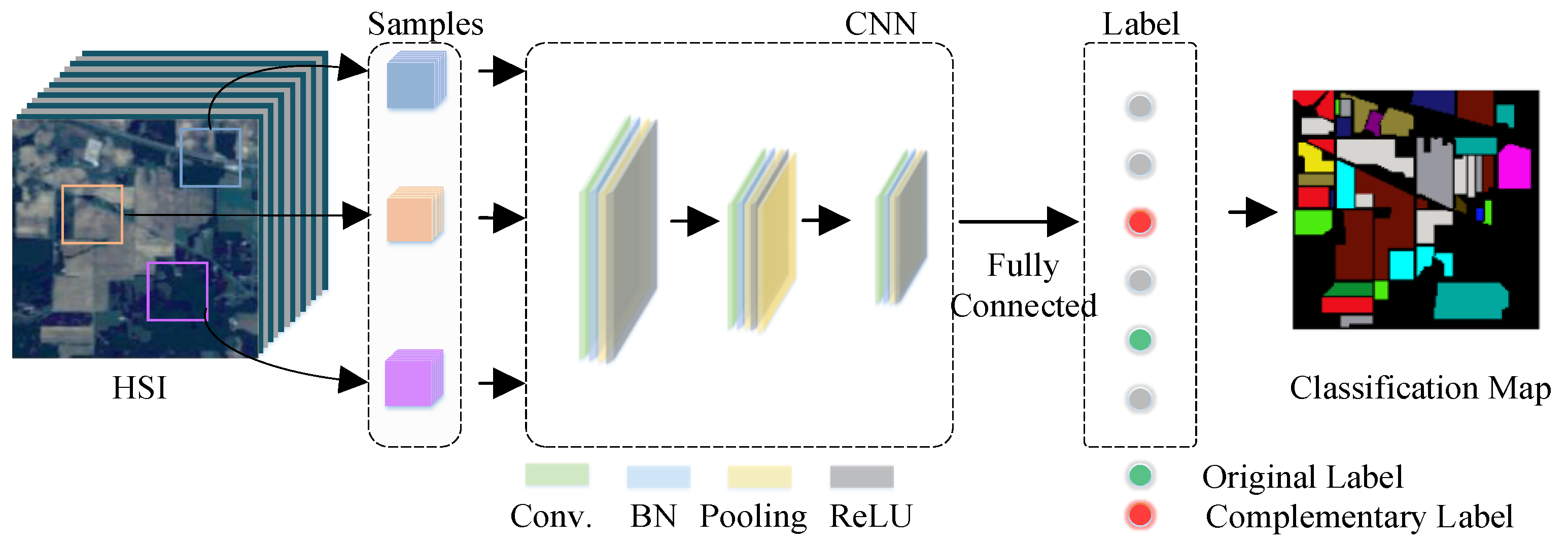
3. CL-Based HSI Classification with Noisy Labels
3.1. CL-Based Deep CNN for HSI Classification
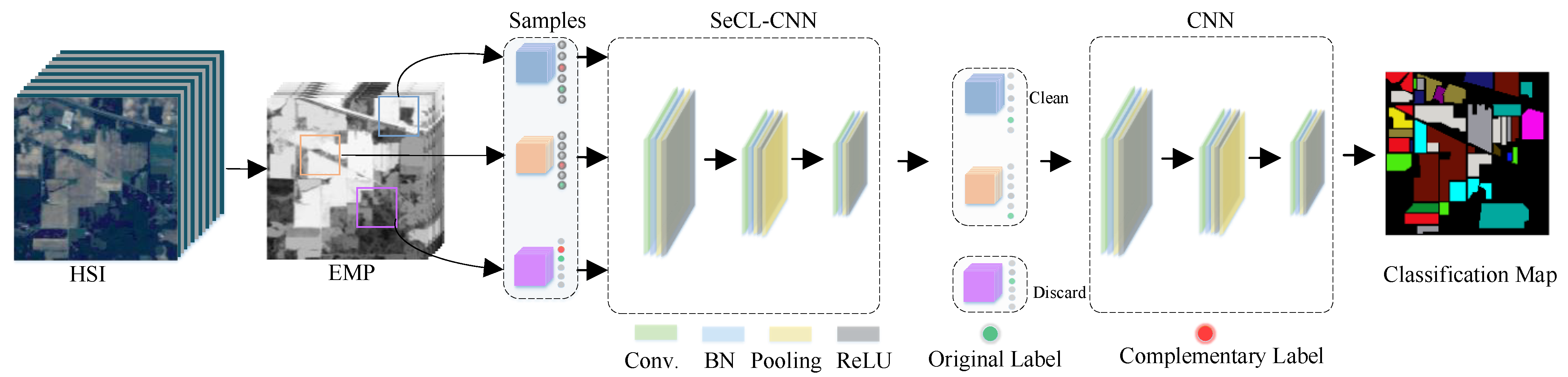
3.2. CL-Based HSI Classification with Noisy Labels
| Algorithm 1 SeCL-CNN for HSI classification with noisy labels |
| 1. Begin 2. Input: Noisy training samples , where is a 3D cube from EMPs of HSI and y is the corresponding label 3. Initialize network 4. For t = 1 to do: Batch (, ) = sample (x, y) from For each x do: Get complementary label using Equation (1) Calculate by Equation (3) Update f by minimizing 5. For t = 1 to do: Batch (, ) = sample (x, y) from , if For each x do: Get complementary label using Equation (1) Calculate by Equation (3) Update f by minimizing 6. (, ) = sample (x, y) from , if 7. Initialize network 8. For t = 1 to do: Batch (, ) = sample (x, y) from (, ) For each x do: Calculate by Equation (2) Update f by minimizing 9. Output: network and filtered dataset (, ) 10. End |
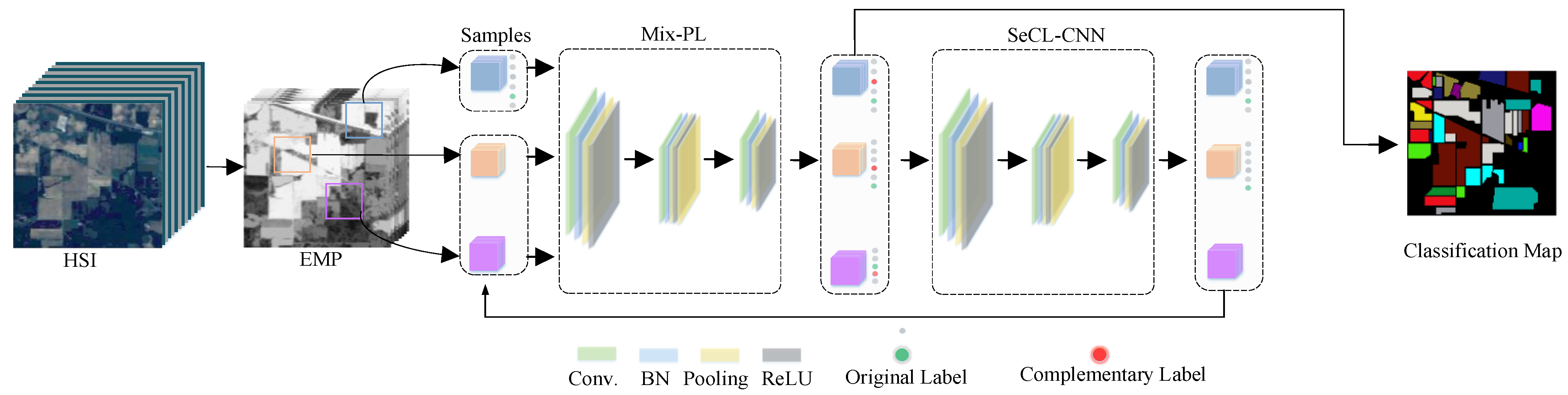
4. CL-Based Semi-Supervised HSI Classification
4.1. Pseudo-Label for HSI Semi-Supervised Classification
4.2. Combining Mixup and Pseudo-Label for HSI Semi-Supervised Classification
4.3. Combining CL and Mix-PL for HSI Semi-Supervised Classification
| Algorithm 2 Mix-PL-CL for HSI semi-supervised classification |
| 1. Begin 2. Input: labeled training set , unlabeled training set 3. Initialize network 4. For i = 1 to . do: 5. For t = 1 to do: For each do: Sample from Calculate supervised loss by Equation (8) Sample from permutation () Get by Equation (11) Calculate unsupervised loss by Equation (12) Update by minimizing Equation (13) 6. For each do: 7. 8. , 9. Output: network 10. End |
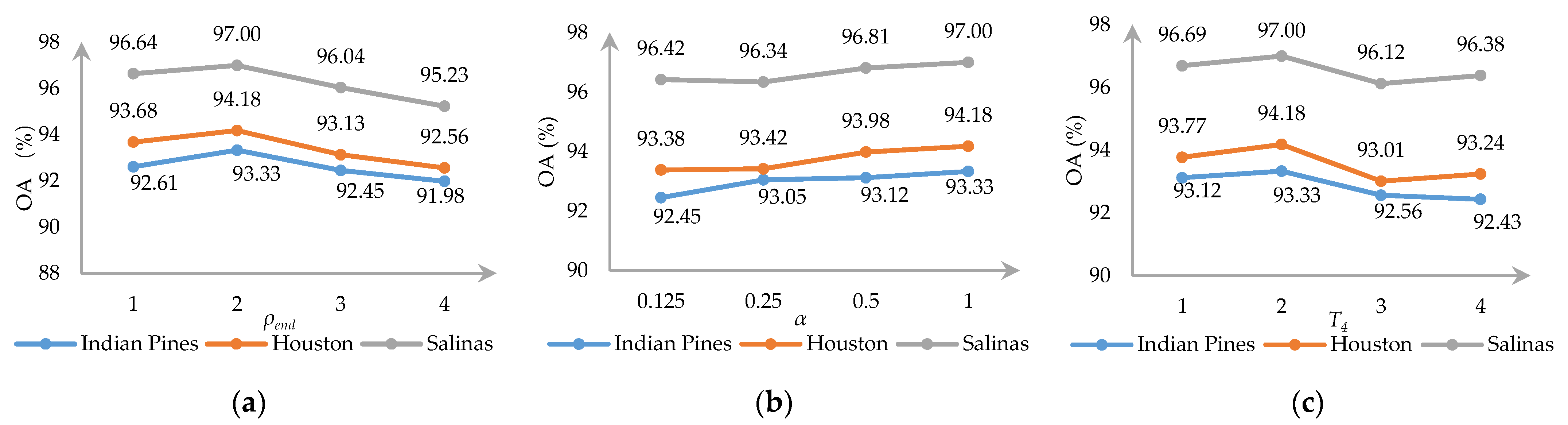
5. Results
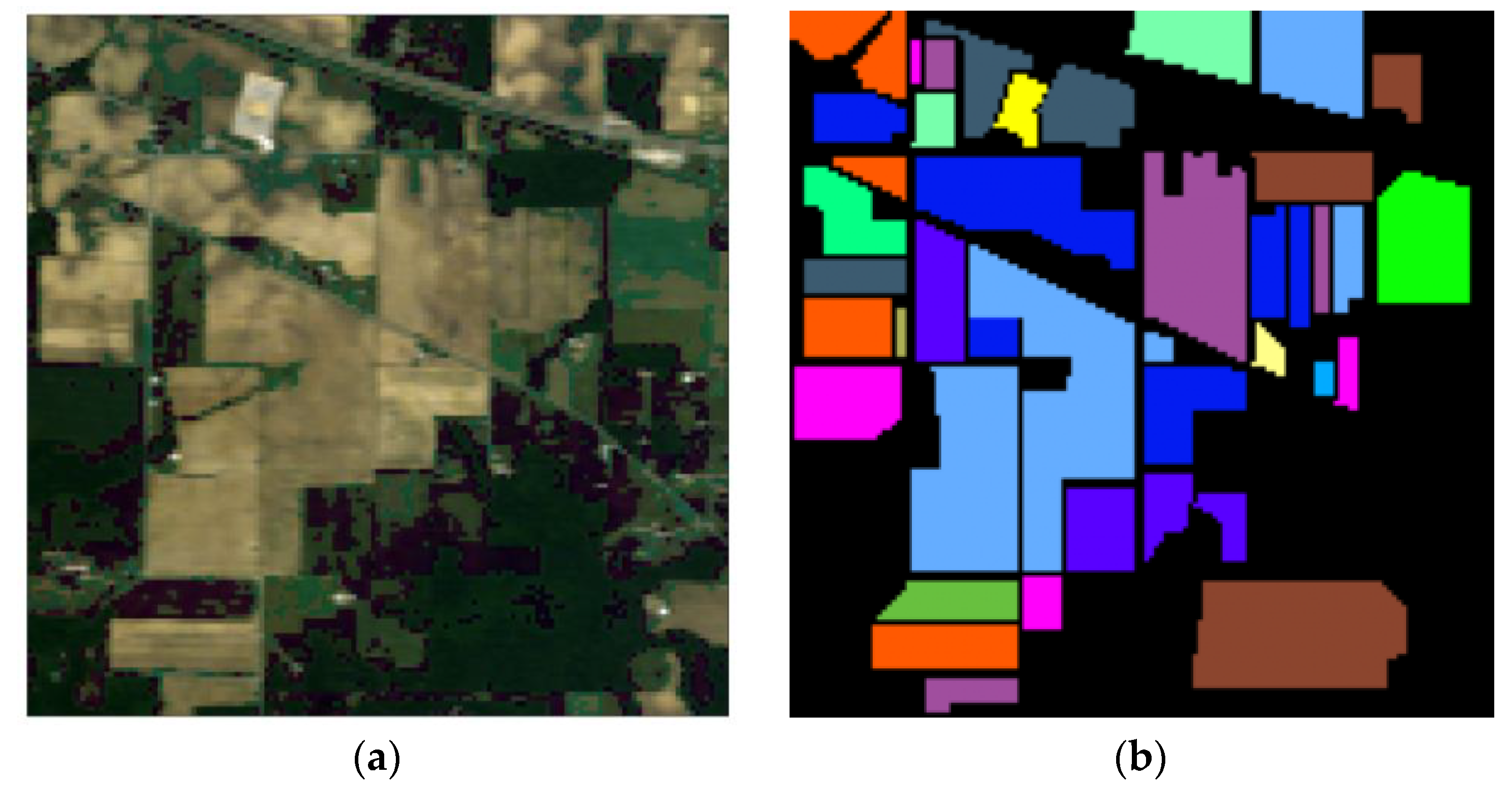
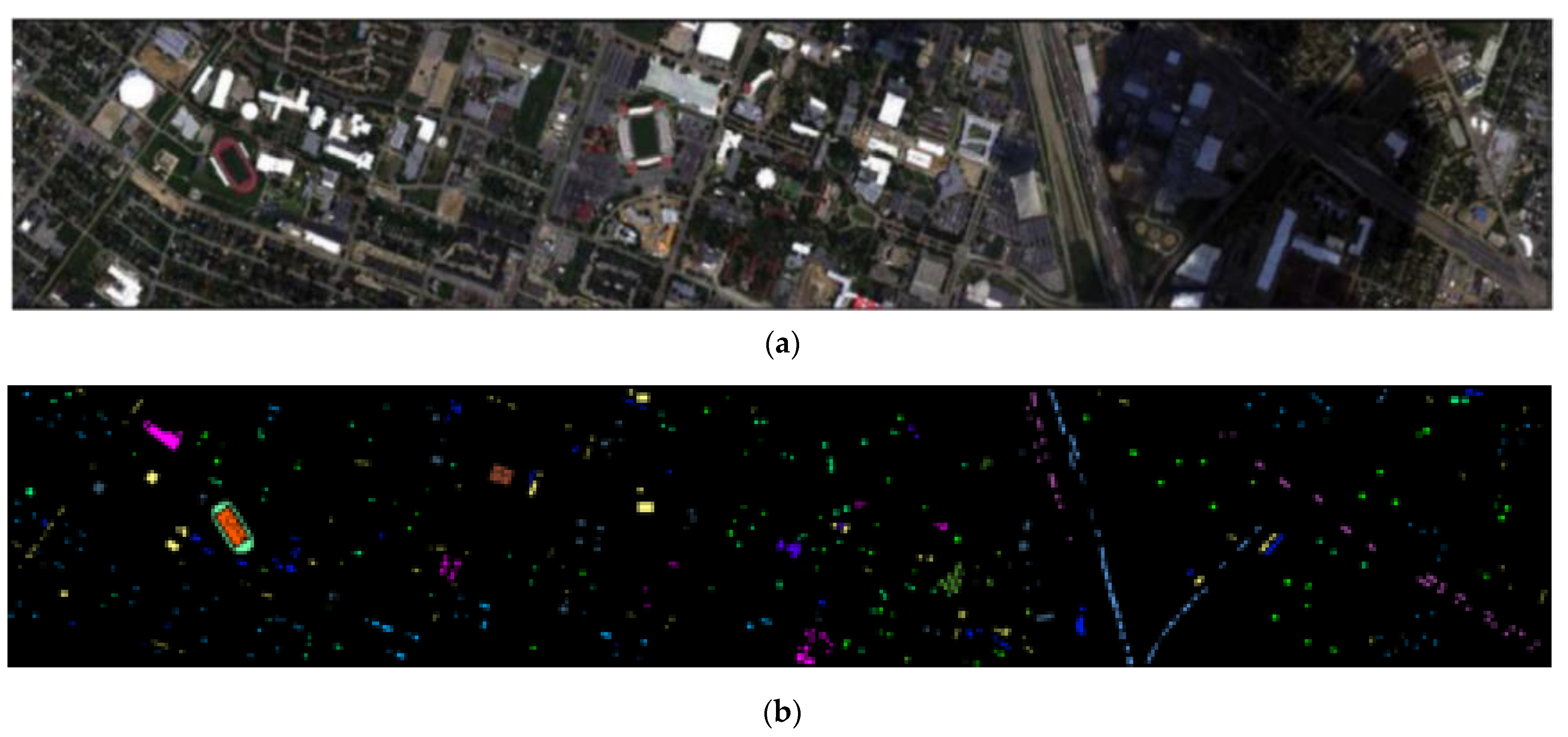
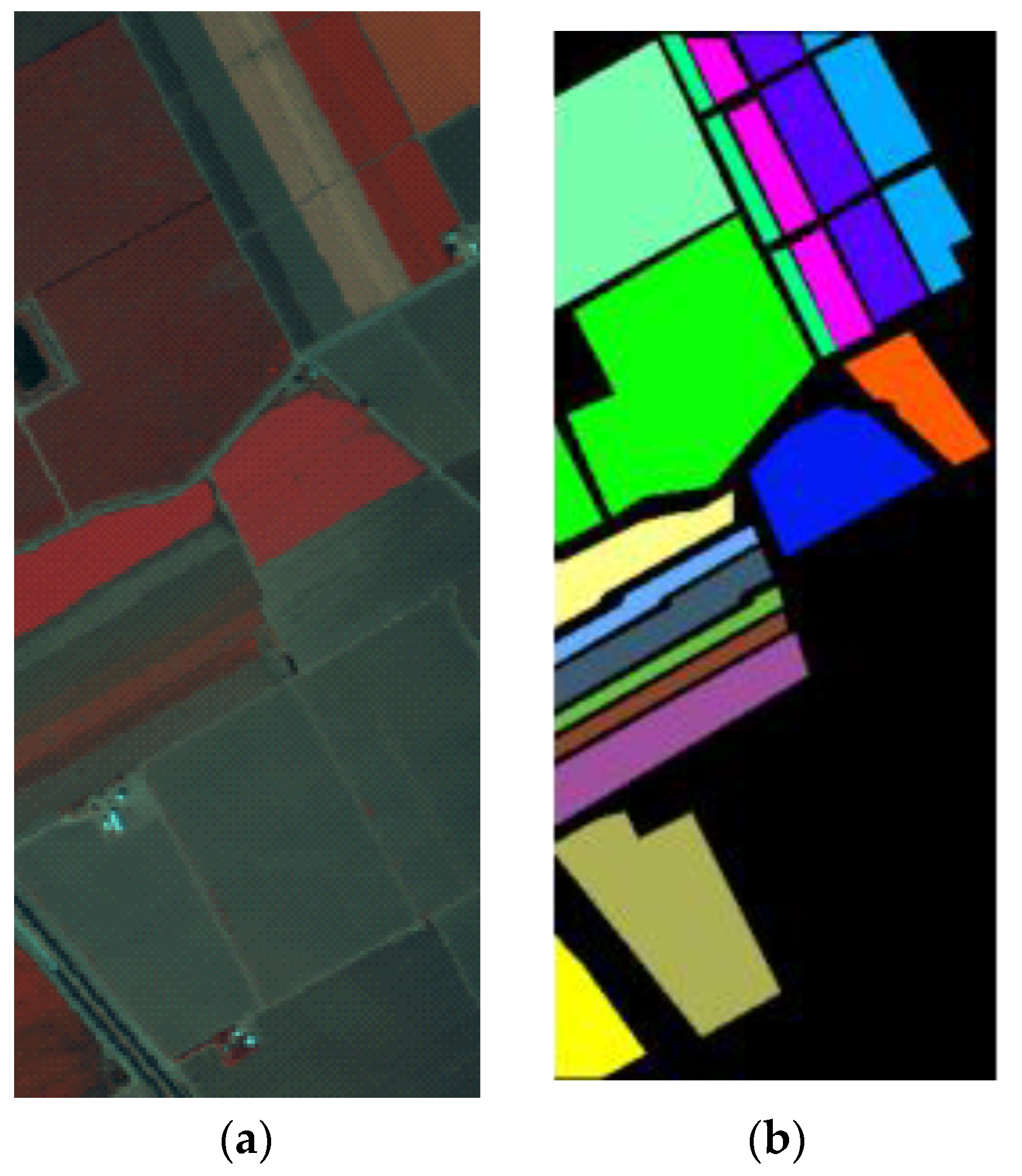
5.1. Datasets Description
5.2. Experimental Setup
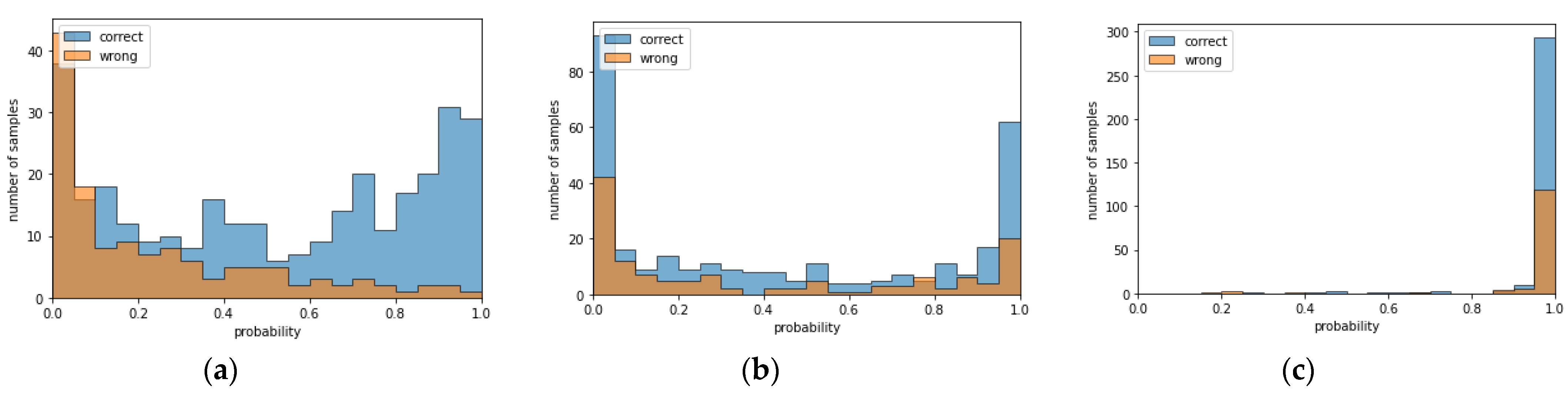
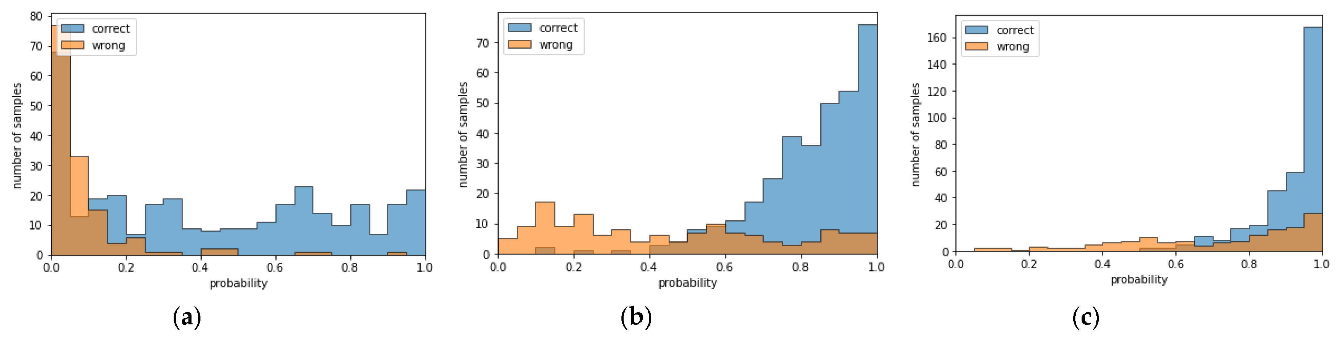
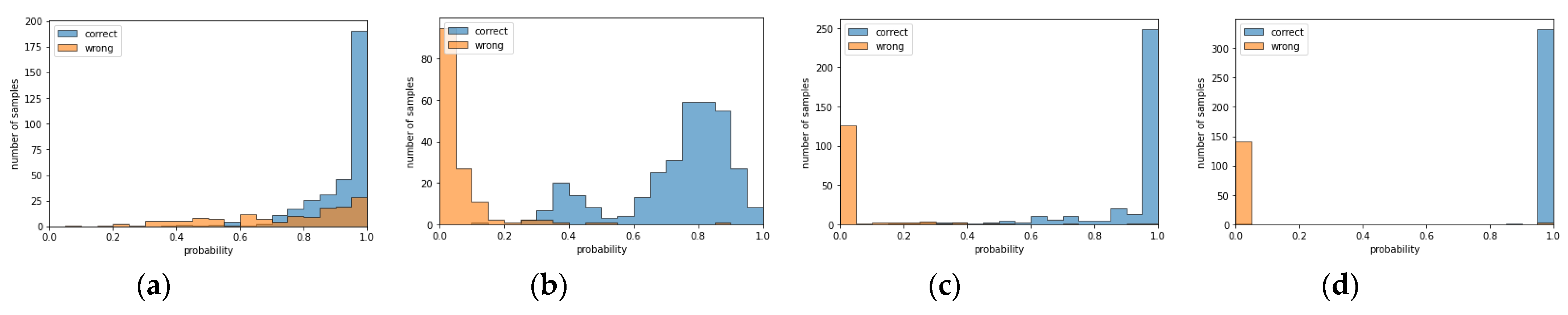
5.3. Results of HSI Classification with Noisy Labels
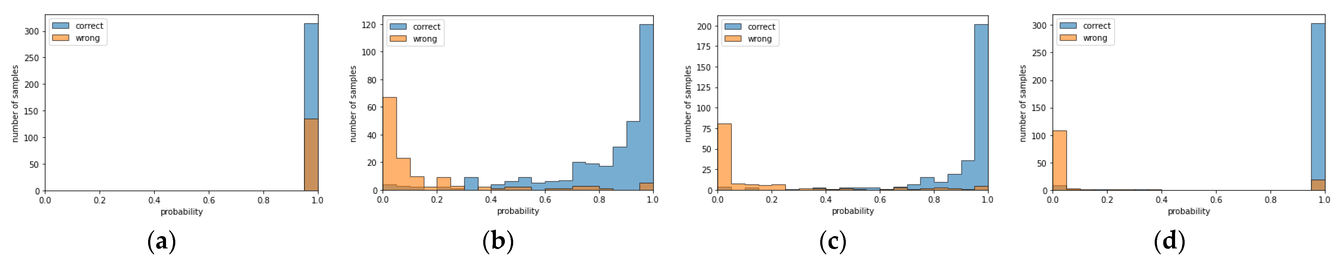
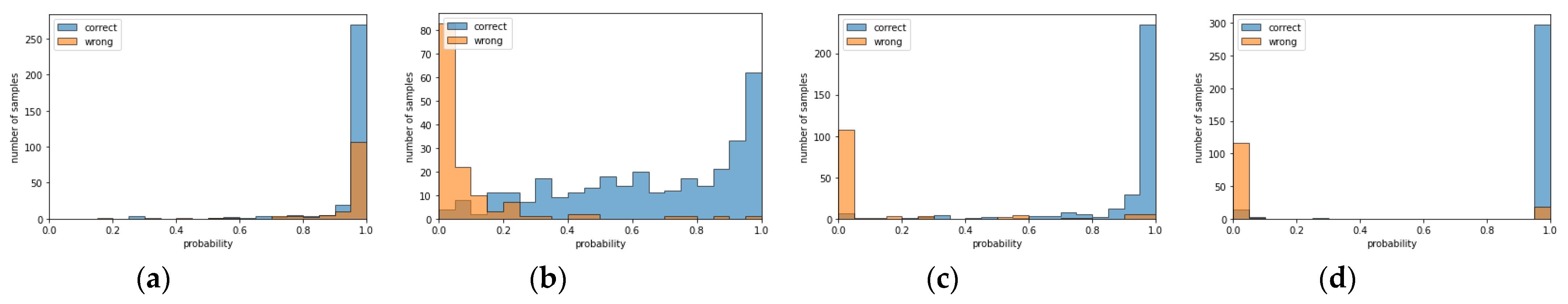
5.4. Results of HSI Semi-Supervised Classification
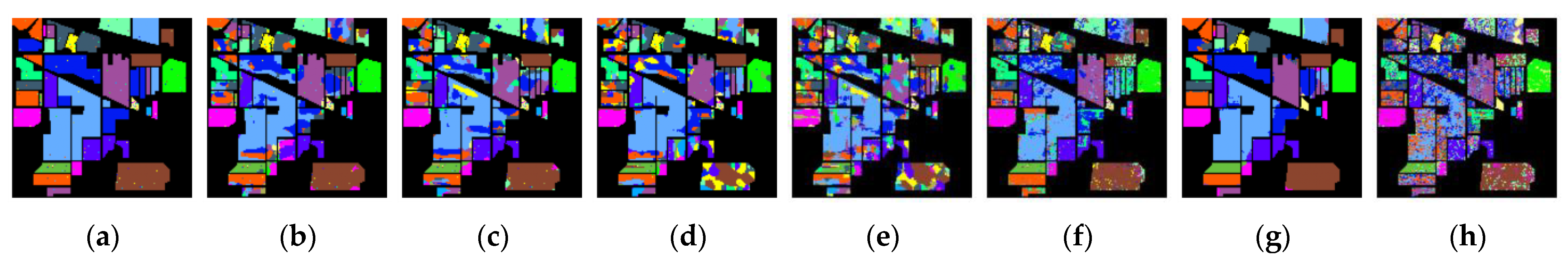
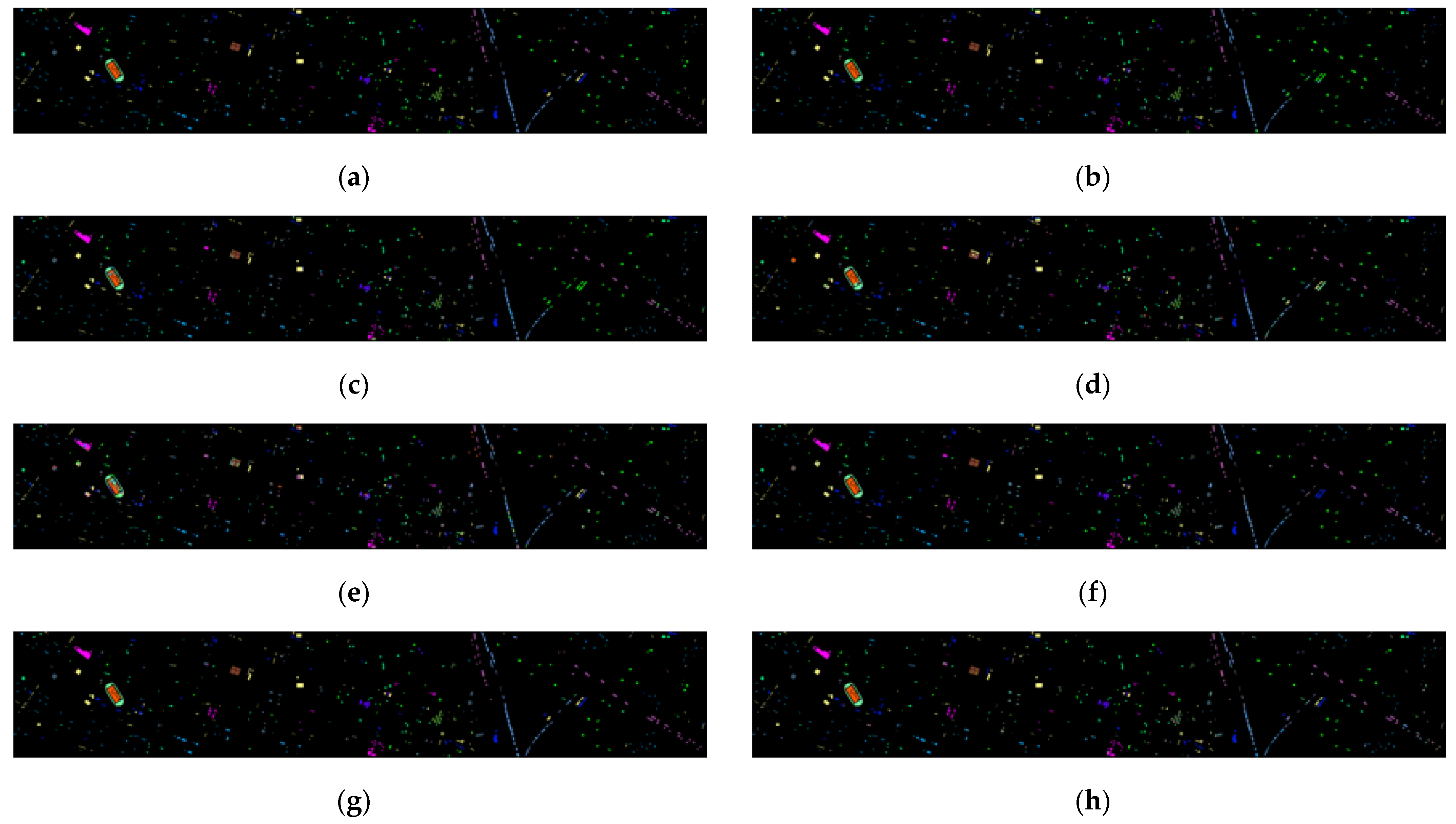
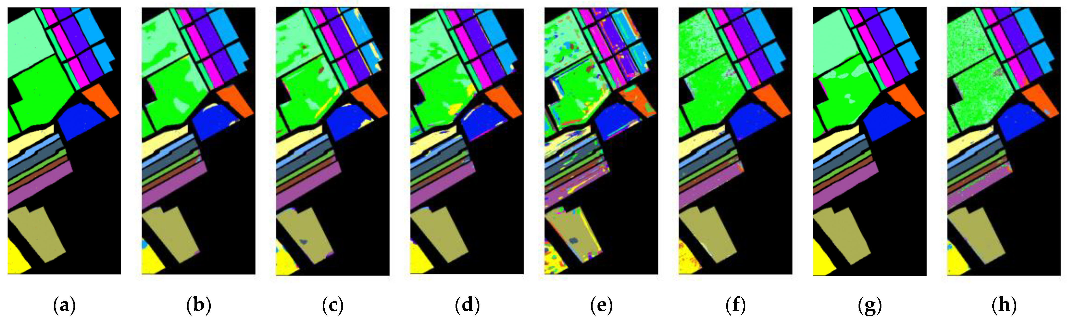
5.5. Classification Maps of Different Classification Methods
6. Conclusions
Author Contributions
Funding
Institutional Review Board Statement
Informed Consent Statement
Data Availability Statement
Conflicts of Interest
Appendix A. Detailed Classification Results

| Noise Ratio | Class | RBF-SVM | EMP-SVM | CNN | MCNN-CP | CNN-Lq | DP-CNN | KSDP-CNN | SSDP-CNN | SeCL-CNN |
|---|---|---|---|---|---|---|---|---|---|---|
| 30% | OA (%) | 4.53 | 3.54 | 2.87 | 68.16 ± 3.27 | 66.36 ± 5.14 | 2.82 | 2.64 | 72.88 ± 2.47 | 2.94 |
| AA (%) | 2.77 | 2.19 | 1.97 | 72.21 ± 2.06 | 3.01 | 1.68 | 1.73 | 82.62 ± 1.24 | 2.07 | |
| K × 100 | 49.94 ± 4.53 | 3.70 | 3.00 | 64.30 ± 3.48 | 5.51 | 3.01 | 2.84 | 69.86 ± 2.67 | 3.21 | |
 | 11.92 | 9.04 | 10.25 | 73.21 ± 11.23 | 9.27 | 9.46 | 5.00 | 95.62 ± 5.63 | 1.88 | |
 | 8.13 | 7.34 | 5.36 | 61.56 ± 4.78 | 7.74 | 5.87 | 7.61 | 58.36 ± 5.73 | 6.82 | |
 | 10.50 | 9.97 | 5.48 | 57.28 ± 10.34 | 9.00 | 8.87 | 10.58 | 63.62 ± 8.71 | 15.91 | |
 | 9.38 | 10.14 | 6.21 | 77.94 ± 6.91 | 6.68 | 9.03 | 8.50 | 85.51 ± 4.41 | 8.20 | |
 | 4.99 | 2.86 | 7.01 | 75.77 ± 6.69 | 8.30 | 11.77 | 10.95 | 80.04 ± 10.93 | 9.93 | |
 | 8.03 | 7.45 | 5.83 | 69.90 ± 6.54 | 6.43 | 9.35 | 12.68 | 79.06 ± 10.69 | 19.23 | |
 | 7.05 | 3.53 | 22.31 | 67.56 ± 18.22 | 18.46 | 20.12 | 16.06 | 89.24 ± 15.07 | 2.31 | |
 | 4.80 | 4.29 | 8.68 | 81.64 ± 5.52 | 5.94 | 8.17 | 3.32 | 95.31 ± 5.07 | 4.75 | |
 | 20.00 | 14.97 | 24.98 | 88.17 ± 19.84 | 23.32 | 13.27 | 9.17 | 96.00 ± 8.00 | 6.00 | |
 | 13.28 | 10.70 | 10.12 | 69.47 ± 8.12 | 10.39 | 8.95 | 6.75 | 72.65 ± 7.27 | 7.08 | |
 | 18.99 | 15.36 | 9.11 | 62.66 ± 11.56 | 15.31 | 8.87 | 9.60 | 69.47 ± 9.33 | 8.31 | |
 | 9.41 | 11.00 | 5.50 | 67.21 ± 4.62 | 7.59 | 6.94 | 8.46 | 70.94 ± 6.03 | 6.76 | |
 | 2.14 | 1.72 | 10.11 | 75.16 ± 8.37 | 10.19 | 4.93 | 5.01 | 91.60 ± 6.86 | 5.61 | |
 | 8.75 | 5.56 | 9.75 | 79.68 ± 8.67 | 11.75 | 7.13 | 6.02 | 90.56 ± 5.63 | 5.16 | |
 | 10.52 | 10.89 | 8.88 | 72.77 ± 9.95 | 9.70 | 7.93 | 7.88 | 85.45 ± 7.05 | 9.43 | |
 | 9.14 | 8.93 | 9.94 | 75.34 ± 13.95 | 5.72 | 4.23 | 4.51 | 93.65 ± 4.32 | 4.65 |
| Noise Ratio | Class | RBF-SVM | EMP-SVM | CNN | MCNN-CP | CNN-Lq | DP-CNN | KSDP-CNN | SSDP-CNN | SeCL-CNN |
|---|---|---|---|---|---|---|---|---|---|---|
| 30% | OA (%) | 1.91 | 1.62 | 1.96 | 75.58 ± 2.63 | 2.12 | 2.36 | 2.27 | 78.16 ± 2.00 | 2.51 |
| AA (%) | 1.33 | 1.54 | 1.92 | 76.02 ± 2.33 | 2.28 | 2.22 | 2.26 | 79.49 ± 1.49 | 2.45 | |
| K × 100 | 2.06 | 1.75 | 2.11 | 73.63 ± 2.84 | 2.29 | 2.53 | 2.93 | 76.40 ± 2.13 | 2.72 | |
| | 7.10 | 7.70 | 8.39 | 72.72 ± 14.54 | 7.02 | 7.17 | 7.49 | 78.76 ± 7.19 | 7.49 | |
| | 6.67 | 8.59 | 8.57 | 76.07 ± 11.70 | 13.05 | 9.09 | 8.93 | 71.43 ± 5.64 | 8.26 | |
| | 0.67 | 1.05 | 10.69 | 85.27 ± 5.64 | 9.46 | 7.56 | 7.03 | 88.85 ± 7.78 | 5.75 | |
| | 3.12 | 3.06 | 8.32 | 83.55 ± 6.19 | 5.55 | 5.86 | 5.24 | 84.76 ± 2.86 | 2.70 | |
| | 4.59 | 3.98 | 5.00 | 85.28 ± 5.68 | 8.44 | 6.37 | 5.52 | 93.01 ± 5.57 | 4.57 | |
| | 10.14 | 8.33 | 5.96 | 70.15 ± 7.72 | 8.18 | 6.80 | 5.17 | 72.95 ± 6.82 | 13.12 | |
| | 6.74 | 9.29 | 5.81 | 68.15 ± 8.11 | 5.72 | 5.64 | 7.71 | 75.54 ± 4.45 | 7.18 | |
| | 7.20 | 6.74 | 7.38 | 63.07 ± 5.14 | 10.62 | 57.30 ± 5.83 | 7.89 | 67.91 ± 8.33 | 8.90 | |
| | 5.44 | 8.98 | 8.36 | 67.24 ± 8.96 | 7.05 | 8.57 | 7.81 | 68.35 ± 11.48 | 8.14 | |
| | 17.97 | 11.38 | 12.98 | 73.32 ± 9.21 | 9.34 | 13.12 | 13.90 | 72.90 ± 12.55 | 16.92 | |
| | 6.40 | 5.59 | 5.35 | 84.00 ± 5.82 | 7.49 | 6.30 | 7.31 | 74.06 ± 7.25 | 11.42 | |
| | 10.50 | 13.84 | 8.06 | 73.71 ± 10.65 | 8.75 | 9.86 | 7.80 | 77.22 ± 6.83 | 8.47 | |
| | 5.51 | 5.46 | 11.14 | 77.16 ± 9.11 | 7.64 | 10.97 | 6.31 | 79.68 ± 8.32 | 3.00 | |
| | 1.03 | 2.09 | 9.56 | 78.30 ± 10.50 | 11.25 | 7.96 | 4.45 | 95.58 ± 5.17 | 7.64 | |
| | 2.09 | 2.90 | 5.81 | 82.31 ± 4.69 | 77.628.58 | 8.18 | 4.38 | 91.33 ± 5.98 | 8.52 |
| Noise Ratio | Class | RBF-SVM | EMP-SVM | CNN | MCNN-CP | CNN-Lq | DP-CNN | KSDP-CNN | SSDP-CNN | SeCL-CNN |
|---|---|---|---|---|---|---|---|---|---|---|
| 30% | OA (%) | 2.05 | 2.02 | 2.30 | 84.53 ± 2.79 | 1.92 | 2.38 | 3.32 | 89.76 ± 1.67 | 2.31 |
| AA (%) | 1.09 | 92.23 ± 1.35 | 75.44 ± 1.24 | 85.27 ± 2.95 | 93.77 ± 1.57 | 2.01 | 1.17 | 92.86 ± 1.40 | 1.48 | |
| K × 100 | 2.22 | 2.21 | 2.48 | 82.84 ± 3.07 | 2.13 | 2.63 | 2.53 | 88.62 ± 1.85 | 2.55 | |
| | 0.93 | 0.46 | 9.77 | 88.88 ± 7.36 | 2.95 | 3.05 | 2.74 | 97.29 ± 3.31 | 0.08 | |
| | 3.13 | 1.68 | 6.30 | 89.40 ± 4.16 | 5.84 | 5.83 | 6.44 | 93.43 ± 4.84 | 4.05 | |
| | 12.47 | 13.79 | 8.63 | 84.47 ± 9.66 | 8.41 | 9.30 | 9.23 | 89.95 ± 8.86 | 8.47 | |
| | 0.52 | 1.95 | 7.27 | 85.03 ± 8.80 | 2.00 | 3.27 | 3.28 | 94.40 ± 5.75 | 1.10 | |
| | 3.70 | 4.70 | 8.93 | 88.11 ± 3.09 | 4.77 | 6.80 | 6.22 | 91.81 ± 5.91 | 6.76 | |
| | 3.02 | 3.73 | 9.07 | 87.78 ± 9.04 | 3.33 | 8.22 | 7.82 | 97.01 ± 6.42 | 3.50 | |
| | 0.49 | 0.62 | 9.23 | 84.18 ± 10.03 | 7.71 | 8.66 | 6.36 | 92.30 ± 5.07 | 3.30 | |
| | 12.11 | 11.75 | 7.26 | 81.05 ± 4.70 | 6.45 | 6.14 | 10.33 | 77.68 ± 4.84 | 7.55 | |
| | 1.32 | 0.96 | 5.54 | 91.37 ± 8.36 | 1.91 | 3.53 | 2.99 | 96.88 ± 3.44 | 2.00 | |
| | 4.01 | 3.57 | 11.85 | 80.59 ± 10.50 | 10.35 | 5.63 | 6.38 | 92.30 ± 5.07 | 8.42 | |
| | 3.91 | 1.09 | 4.90 | 81.09 ± 8.77 | 7.21 | 6.15 | 5.72 | 93.63 ± 6.53 | 5.56 | |
| | 0.52 | 0.12 | 11.29 | 87.65 ± 4.66 | 2.19 | 7.88 | 4.08 | 96.85 ± 6.34 | 1.85 | |
| | 0.67 | 0.75 | 8.03 | 87.10 ± 7.72 | 2.17 | 7.71 | 3.16 | 97.42 ± 3.86 | 1.55 | |
| | 2.51 | 7.17 | 7.58 | 84.48 ± 8.40 | 7.94 | 6.87 | 6.02 | 94.28 ± 5.18 | 7.26 | |
| | 57.38 ± 10.00 | 63.62 ± 9.53 | 67.82 ± 5.42 | 78.56 ± 6.13 | 82.27 ± 10.23 | 82.31 ± 4.92 | 4.99 | 85.07 ± 8.89 | 86.53 ± 6.53 | |
| | 5.09 | 92.69 ± 4.83 | 73.06 ± 10.22 | 84.53 ± 9.32 | 4.36 | 91.22 ± 4.91 | 92.98 ± 3.49 | 95.48 ± 2.51 | 95.43 ± 3.50 |
| N | Class | EMP-CNN | MCNN-CP | LP | LapSVM | EMP-LapSVM | PL | AROC-DP | Mix-PL | CL-MixPL |
|---|---|---|---|---|---|---|---|---|---|---|
| 25 | OA (%) | 91.78 ± 2.22 | 92.74 ± 1.49 | 58.12 ± 1.33 | 61.27 ± 1.27 | 85.09 ± 2.34 | 92.87 ± 2.30 | 92.30 ± 1.72 | 93.12 ± 3.28 | 93.33 ± 2.29 |
| AA (%) | 94.95 ± 1.20 | 96.19 ± 0.74 | 67.86 ± 1.27 | 71.60 ± 1.64 | 90.57 ± 1.43 | 95.35 ± 1.26 | 95.55 ± 0.77 | 95.37 ± 1.27 | 95.74 ± 1.11 | |
| K × 100 | 90.60 ± 2.52 | 91.71 ± 1.69 | 52.73 ± 1.40 | 56.26 ± 1.46 | 83.07 ± 2.61 | 91.83 ± 2.62 | 91.20 ± 1.95 | 92.12 ± 2.71 | 92.35 ± 2.61 | |
| | 100.0 ± 0.00 | 100.0 ± 0.00 | 86.30 ± 10.34 | 88.31 ± 11.63 | 98.18 ± 2.80 | 99.00 ± 3.00 | 100.0 ± 0.00 | 98.50 ± 3.20 | 100.0 ± 0.00 | |
| | 80.86 ± 7.85 | 88.62 ± 3.78 | 31.90 ± 5.17 | 40.10 ± 4.65 | 79.24 ± 3.76 | 83.79 ± 6.37 | 85.36 ± 3.30 | 84.28 ± 6.57 | 86.62 ± 5.90 | |
| | 91.79 ± 4.89 | 90.33 ± 4.92 | 42.32 ± 6.27 | 50.78 ± 7.29 | 84.04 ± 4.62 | 90.59 ± 7.37 | 89.28 ± 5.67 | 90.96 ± 7.20 | 90.23 ± 7.45 | |
| | 98.42 ± 2.03 | 99.25 ± 0.92 | 63.26 ± 6.25 | 68.26 ± 10.47 | 92.61 ± 7.07 | 98.45 ± 1.62 | 99.25 ± 1.26 | 98.25 ± 1.54 | 99.47 ± 0.88 | |
| | 90.89 ± 6.28 | 95.67 ± 2.89 | 79.28 ± 4.95 | 78.79 ± 3.89 | 86.59 ± 2.98 | 89.86 ± 5.47 | 91.98 ± 3.07 | 89.93 ± 5.47 | 91.51 ± 4.71 | |
| | 98.13 ± 1.94 | 97.85 ± 1.61 | 85.64 ± 4.07 | 84.50 ± 5.19 | 90.28 ± 5.56 | 98.60 ± 2.12 | 95.59 ± 14.26 | 98.63 ± 2.13 | 96.04 ± 3.62 | |
| | 100.0 ± 0.00 | 100.0 ± 0.00 | 92.76 ± 6.54 | 92.92 ± 4.71 | 94.87 ± 5.16 | 100.0 ± 0.00 | 100.0 ± 0.00 | 100.0 ± 0.00 | 100.0 ± 0.00 | |
| | 100.0 ± 0.00 | 99.95 ± 0.14 | 80.95 ± 3.24 | 85.99 ± 3.15 | 99.78 ± 0.38 | 100.0 ± 0.00 | 100.0 ± 0.00 | 100.0 ± 0.00 | 100.0 ± 0.00 | |
| | 100.0 ± 0.00 | 100.0 ± 0.00 | 69.50 ± 20.91 | 87.00 ± 14.0 | 100.0 ± 0.00 | 100.0 ± 0.00 | 100.0 ± 0.00 | 100.0 ± 0.00 | 100.0 ± 0.00 | |
| | 87.75 ± 4.33 | 92.98 ± 5.08 | 61.58 ± 7.58 | 60.81 ± 5.43 | 86.82 ± 3.81 | 85.67 ± 6.03 | 88.69 ± 5.52 | 85.16 ± 5.71 | 86.96 ± 5.66 | |
| | 92.51 ± 5.45 | 87.79 ± 3.82 | 55.30 ± 5.84 | 55.53 ± 4.01 | 78.82 ± 6.77 | 95.12 ± 5.21 | 91.03 ± 4.21 | 95.81 ± 5.08 | 95.73 ± 5.17 | |
| | 86.31 ± 6.53 | 90.56 ± 2.33 | 39.49 ± 4.26 | 43.06 ± 7.25 | 83.10 ± 5.44 | 92.87 ± 4.82 | 90.57 ± 2.54 | 93.39 ± 4.86 | 90.71 ± 4.19 | |
| | 99.93 ± 0.21 | 99.41 ± 1.42 | 93.22 ± 2.07 | 93.42 ± 3.11 | 97.46 ± 0.94 | 99.83 ± 0.37 | 99.88 ± 0.36 | 99.89 ± 0.34 | 100.0 ± 0.00 | |
| | 97.95 ± 3.78 | 98.82 ± 1.83 | 76.00 ± 8.64 | 79.62 ± 8.09 | 89.93 ± 8.17 | 97.59 ± 2.11 | 98.81 ± 0.78 | 97.60 ± 2.12 | 96.94 ± 2.53 | |
| | 95.59 ± 4.25 | 98.10 ± 2.92 | 33.66 ± 3.73 | 44.90 ± 7.45 | 89.82 ± 3.19 | 96.54 ± 3.66 | 99.10 ± 1.26 | 96.46 ± 3.59 | 98.74 ± 2.00 | |
| | 99.13 ± 1.16 | 99.67 ± 0.66 | 96.30 ± 3.41 | 91.60 ± 5.44 | 97.58 ± 3.51 | 97.73 ± 2.27 | 99.18 ± 1.10 | 97.12 ± 2.39 | 98.94 ± 0.97 |
| N | Class | EMP-CNN | MCNN-CP | LP | LapSVM | EMP-LapSVM | PL | AROC-DP | Mix-PL | Mix-PL-CL |
|---|---|---|---|---|---|---|---|---|---|---|
| 25 | OA (%) | 92.05 ± 0.82 | 93.44 ± 0.99 | 79.86 ± 0.88 | 82.30 ± 1.04 | 86.52 ± 1.24 | 93.39 ± 1.33 | 93.48 ± 1.15 | 93.77 ± 0.95 | 94.18 ± 0.82 |
| AA (%) | 92.86 ± 0.76 | 94.53 ± 0.98 | 80.37 ± 0.85 | 82.55 ± 1.18 | 87.54 ± 1.24 | 94.23 ± 1.28 | 94.43 ± 1.16 | 94.75 ± 0.89 | 94.98 ± 0.86 | |
| K × 100 | 91.42 ± 0.89 | 92.91 ± 1.07 | 78.22 ± 0.94 | 80.86 ± 1.13 | 85.43 ± 1.34 | 92.86 ± 1.44 | 92.95 ± 1.24 | 93.27 ± 1.02 | 93.71 ± 0.89 | |
| | 90.86 ± 5.39 | 91.90 ± 5.62 | 94.15 ± 4.56 | 94.42 ± 4.26 | 92.58 ± 4.72 | 93.05 ± 3.99 | 91.96 ± 5.11 | 91.43 ± 5.30 | 91.85 ± 4.73 | |
| | 87.25 ± 8.23 | 97.15 ± 2.41 | 95.70 ± 1.64 | 94.38 ± 2.90 | 95.13 ± 2.34 | 87.23 ± 8.91 | 94.66 ± 5.64 | 85.33 ± 8.43 | 88.51 ± 7.70 | |
| | 98.74 ± 0.96 | 99.33 ± 0.45 | 98.14 ± 1.30 | 97.27 ± 2.02 | 97.86 ± 2.19 | 99.53 ± 0.66 | 98.95 ± 0.66 | 99.71 ± 0.34 | 99.82 ± 0.19 | |
| | 94.14 ± 2.28 | 98.65 ± 1.71 | 97.10 ± 2.69 | 95.96 ± 3.26 | 92.03 ± 3.28 | 95.36 ± 5.07 | 96.59 ± 2.91 | 97.46 ± 3.02 | 97.72 ± 2.33 | |
| | 98.75 ± 1.13 | 99.94 ± 0.18 | 96.65 ± 1.24 | 96.62 ± 1.09 | 97.59 ± 1.75 | 99.61 ± 0.69 | 99.72 ± 0.75 | 99.82 ± 0.55 | 99.80 ± 0.55 | |
| | 93.13 ± 5.02 | 98.07 ± 3.88 | 95.33 ± 2.76 | 93.12 ± 3.02 | 96.95 ± 3.07 | 95.54 ± 4.21 | 97.28 ± 3.87 | 96.94 ± 3.93 | 96.87 ± 4.00 | |
| | 85.42 ± 3.02 | 85.81 ± 4.21 | 71.25 ± 5.58 | 77.62 ± 6.82 | 84.94 ± 3.26 | 91.86 ± 4.41 | 89.32 ± 1.67 | 91.64 ± 3.08 | 91.95 ± 3.21 | |
| | 82.42 ± 3.06 | 79.82 ± 5.79 | 65.64 ± 4.19 | 65.37 ± 8.14 | 75.27 ± 4.68 | 79.65 ± 6.82 | 80.04 ± 6.81 | 83.18 ± 5.60 | 81.97 ± 5.40 | |
| | 90.48 ± 3.76 | 87.50 ± 5.33 | 66.94 ± 3.89 | 74.87 ± 6.84 | 80.51 ± 3.80 | 92.66 ± 5.88 | 91.96 ± 4.00 | 94.98 ± 2.78 | 95.56 ± 3.08 | |
| | 97.69 ± 2.59 | 96.90 ± 2.21 | 74.52 ± 3.93 | 80.49 ± 5.65 | 86.56 ± 6.10 | 99.07 ± 1.05 | 96.49 ± 7.75 | 98.09 ± 2.30 | 97.50 ± 3.95 | |
| | 93.43 ± 3.20 | 96.39 ± 2.60 | 67.87 ± 3.59 | 72.00 ± 3.75 | 79.13 ± 3.20 | 96.05 ± 2.63 | 93.93 ± 3.98 | 96.15 ± 2.29 | 97.03 ± 1.99 | |
| | 90.25 ± 4.98 | 89.27 ± 4.15 | 57.47 ± 5.50 | 62.59 ± 6.42 | 67.76 ± 7.25 | 89.80 ± 5.89 | 89.99 ± 4.89 | 89.10 ± 6.43 | 91.05 ± 5.10 | |
| | 92.30 ± 3.86 | 97.23 ± 2.82 | 28.41 ± 5.02 | 39.92 ± 8.41 | 70.69 ± 4.74 | 94.21 ± 5.23 | 95.61 ± 3.49 | 97.43 ± 1.61 | 95.10 ± 4.54 | |
| | 99.76 ± 0.50 | 100.0 ± 0.00 | 97.07 ± 2.29 | 95.32 ± 4.30 | 96.55 ± 2.41 | 99.92 ± 0.16 | 100.0 ± 0.00 | 100.0 ± 0.00 | 99.95 ± 0.15 | |
| | 98.19 ± 2.70 | 100.0 ± 0.00 | 99.33 ± 0.72 | 98.33 ± 1.00 | 99.58 ± 0.59 | 100.0 ± 0.00 | 99.92 ± 0.19 | 99.98 ± 0.05 | 99.98 ± 0.05 |
| N | Class | EMP-CNN | MCNN-CP | LP | LapSVM | EMP-LapSVM | PL | AROC-DP | Mix-PL | CL-MixPL |
|---|---|---|---|---|---|---|---|---|---|---|
| 25 | OA (%) | 94.95 ± 2.46 | 96.17 ± 0.98 | 84.13 ± 1.19 | 86.12 ± 1.96 | 91.93 ± 1.71 | 95.97 ± 2.25 | 96.18 ± 1.72 | 96.69 ± 0.71 | 97.00 ± 0.85 |
| AA (%) | 98.24 ± 0.80 | 98.37 ± 0.37 | 91.91 ± 0.44 | 92.01 ± 1.01 | 95.18 ± 1.10 | 98.49 ± 0.82 | 98.63 ± 0.44 | 98.82 ± 0.22 | 98.91 ± 0.30 | |
| K × 100 | 94.40 ± 2.70 | 95.64 ± 0.85 | 82.40 ± 1.30 | 84.59 ± 2.15 | 91.02 ± 1.91 | 95.53 ± 2.48 | 95.76 ± 1.34 | 96.33 ± 0.78 | 96.67 ± 0.94 | |
| | 99.99 ± 0.03 | 100.0 ± 0.00 | 98.07 ± 1.04 | 97.04 ± 1.87 | 99.24 ± 0.60 | 99.89 ± 0.22 | 100.0 ± 0.00 | 100.0 ± 0.00 | 100.0 ± 0.00 | |
| | 98.79 ± 2.60 | 99.92 ± 0.19 | 99.56 ± 0.37 | 96.99 ± 1.59 | 97.95 ± 2.51 | 97.00 ± 5.46 | 99.52 ± 1.78 | 99.02 ± 1.39 | 98.67 ± 2.67 | |
| | 99.97 ± 0.08 | 99.99 ± 0.02 | 95.57 ± 3.00 | 94.29 ± 3.21 | 99.59 ± 0.45 | 99.83 ± 0.27 | 99.37 ± 1.04 | 99.94 ± 0.17 | 99.92 ± 0.17 | |
| | 99.89 ± 0.31 | 99.43 ± 0.42 | 98.96 ± 1.41 | 98.86 ± 0.86 | 99.02 ± 1.00 | 99.96 ± 0.13 | 99.94 ± 0.14 | 99.974 ± 0.10 | 99.96 ± 0.07 | |
| | 99.13 ± 0.73 | 97.38 ± 2.04 | 95.41 ± 2.37 | 95.03 ± 2.01 | 96.25 ± 2.71 | 99.12 ± 1.04 | 99.10 ± 1.00 | 99.07 ± 1.02 | 99.50 ± 0.56 | |
| | 100.0 ± 0.00 | 99.98 ± 0.12 | 99.36 ± 0.32 | 98.27 ± 0.97 | 98.60 ± 1.10 | 100.0 ± 0.00 | 100.0 ± 0.00 | 100.0 ± 0.00 | 100.0 ± 0.00 | |
| | 99.80 ± 0.39 | 99.94 ± 0.12 | 99.38 ± 0.38 | 96.88 ± 3.71 | 97.74 ± 2.45 | 100.0 ± 0.00 | 99.55 ± 0.96 | 99.95 ± 0.05 | 100.0 ± 0.01 | |
| | 79.71 ± 11.1 | 88.55 ± 3.07 | 58.83 ± 7.24 | 70.19 ± 9.31 | 82.59 ± 5.53 | 84.16 ± 9.52 | 84.89 ± 4.90 | 87.19 ± 2.88 | 89.03 ± 3.28 | |
| | 99.93 ± 0.20 | 100.0 ± 0.00 | 95.61 ± 1.38 | 95.85 ± 2.14 | 97.98 ± 1.28 | 99.93 ± 0.20 | 100.0 ± 0.00 | 100.0 ± 0.00 | 100.0 ± 0.00 | |
| | 99.98 ± 0.06 | 99.09 ± 0.98 | 86.46 ± 2.36 | 85.37 ± 4.36 | 95.64 ± 2.34 | 99.95 ± 0.09 | 99.85 ± 0.17 | 99.88 ± 0.17 | 99.99 ± 0.02 | |
| | 99.85 ± 0.16 | 99.97 ± 0.06 | 93.51 ± 2.25 | 93.10 ± 2.59 | 96.05 ± 2.69 | 99.86 ± 0.14 | 99.88 ± 0.10 | 99.91 ± 0.13 | 99.88 ± 0.14 | |
| | 99.95 ± 0.12 | 99.78 ± 0.52 | 99.56 ± 0.53 | 99.47 ± 1.02 | 100.0 ± 0.00 | 100.0 ± 0.00 | 100.0 ± 0.00 | 99.99 ± 0.02 | 100.0 ± 0.00 | |
| | 99.73 ± 0.60 | 100.0 ± 0.00 | 96.89 ± 1.95 | 97.71 ± 1.65 | 97.77 ± 1.52 | 99.99 ± 0.03 | 99.89 ± 0.23 | 99.93 ± 0.12 | 99.99 ± 0.03 | |
| | 99.87 ± 0.21 | 99.70 ± 0.39 | 92.95 ± 2.80 | 92.96 ± 3.66 | 92.91 ± 3.26 | 99.45 ± 1.06 | 99.88 ± 0.22 | 99.86 ± 0.27 | 99.89 ± 0.26 | |
| | 95.31 ± 2.43 | 91.35 ± 5.08 | 62.89 ± 5.20 | 64.97 ± 7.42 | 79.42 ± 4.63 | 96.80 ± 3.55 | 96.26 ± 2.58 | 99.37 ± 2.05 | 95.76 ± 3.13 | |
| | 99.95 ± 0.13 | 98.86 ± 1.01 | 97.52 ± 1.41 | 95.14 ± 3.05 | 92.04 ± 5.66 | 99.92 ± 0.24 | 99.94 ± 0.14 | 99.99 ± 0.02 | 99.95 ± 0.09 |
References
- Gevaert, C.M.; Suomalainen, J.; Tang, J.; Kooistra, L. Generation of spectral–temporal response surfaces by combining multispectral satellite and hyperspectral UAV imagery for precision agriculture applications. IEEE J. Sel. Top. Appl. Earth Obs. Remote Sens. 2015, 8, 3140–3146. [Google Scholar] [CrossRef]
- Murphy, R.J.; Schneider, S.; Monteiro, S.T. Consistency of Measurements of Wavelength Position from Hyperspectral Imagery: Use of the Ferric Iron Crystal Field Absorption at ~900 nm as an Indicator of Mineralogy. IEEE Trans. Geosci. Remote Sens. 2013, 52, 2843–2857. [Google Scholar] [CrossRef]
- Koz, A. Ground-Based Hyperspectral Image Surveillance Systems for Explosive Detection: Part I—State of the Art and Challenges. IEEE J. Sel. Top. Appl. Earth Obs. Remote Sens. 2019, 12, 4746–4753. [Google Scholar] [CrossRef]
- Qu, D.-X.; Berry, J.; Calta, N.P.; Crumb, M.F.; Guss, G.; Matthews, M.J. Temperature Measurement of Laser-Irradiated Metals Using Hyperspectral Imaging. Phys. Rev. Appl. 2020, 14, 014031. [Google Scholar] [CrossRef]
- Berné, O.; Helens, A.; Pilleri, P.; Joblin, C. Non-negative matrix factorization pansharpening of hyperspectral data: An application to mid-infrared astronomy. In Proceedings of the 2010 2nd Workshop on Hyperspectral Image and Signal Processing: Evolution in Remote Sensing, Reykjavìk, Iceland, 14–16 June 2010; pp. 1–4. [Google Scholar]
- Cheng, J.-H.; Sun, D.-W.; Pu, H.; Zhu, Z. Development of hyperspectral imaging coupled with chemometric analysis to monitor K value for evaluation of chemical spoilage in fish fillets. Food Chem. 2015, 185, 245–253. [Google Scholar] [CrossRef]
- Chang, C.-I. Hyperspectral Data Exploitation: Theory and Applications; John Wiley & Sons: Hoboken, NJ, USA, 2007. [Google Scholar]
- Bioucas-Dias, J.M.; Plaza, A.; Camps-Valls, G.; Scheunders, P.; Nasrabadi, N.; Chanussot, J. Hyperspectral remote sensing data analysis and future challenges. IEEE Geosci. Remote Sens. Mag. 2013, 1, 6–36. [Google Scholar] [CrossRef] [Green Version]
- Ghamisi, P.; Yokoya, N.; Li, J.; Liao, W.; Liu, S.; Plaza, J.; Rasti, B.; Plaza, A. Advances in hyperspectral image and signal processing: A comprehensive overview of the state of the art. IEEE Geosci. Remote Sens. Mag. 2017, 5, 37–78. [Google Scholar] [CrossRef] [Green Version]
- Fauvel, M.; Tarabalka, Y.; Benediktsson, J.A.; Chanussot, J.; Tilton, J.C. Advances in spectral-spatial classification of hyperspectral images. Proc. IEEE 2012, 101, 652–675. [Google Scholar] [CrossRef] [Green Version]
- Ghamisi, P.; Plaza, J.; Chen, Y.; Li, J.; Plaza, A.J. Advanced spectral classifiers for hyperspectral images: A review. IEEE Geosci. Remote Sens. Mag. 2017, 5, 8–32. [Google Scholar] [CrossRef] [Green Version]
- He, L.; Li, J.; Liu, C.; Li, S. Recent advances on spectral–spatial hyperspectral image classification: An overview and new guidelines. IEEE Trans. Geosci. Remote Sens. 2017, 56, 1579–1597. [Google Scholar] [CrossRef]
- Sowmya, V.; Soman, K.; Hassaballah, M. Hyperspectral image: Fundamentals and advances. In Recent Advances in Computer Vision; Springer: Berlin/Heidelberg, Germany, 2019; pp. 401–424. [Google Scholar]
- Melgani, F.; Bruzzone, L. Classification of hyperspectral remote sensing images with support vector machines. IEEE Trans. Geosci. Remote Sens. 2004, 42, 1778–1790. [Google Scholar] [CrossRef] [Green Version]
- Benediktsson, J.A.; Palmason, J.A.; Sveinsson, J.R. Classification of hyperspectral data from urban areas based on extended morphological profiles. IEEE Trans. Geosci. Remote Sens. 2005, 43, 480–491. [Google Scholar] [CrossRef]
- Dalla Mura, M.; Villa, A.; Benediktsson, J.A.; Chanussot, J.; Bruzzone, L. Classification of hyperspectral images by using extended morphological attribute profiles and independent component analysis. IEEE Geosci. Remote Sens. Lett. 2010, 8, 542–546. [Google Scholar] [CrossRef] [Green Version]
- Chen, Y.; Nasrabadi, N.M.; Tran, T.D. Hyperspectral image classification using dictionary-based sparse representation. IEEE Trans. Geosci. Remote Sens. 2011, 49, 3973–3985. [Google Scholar] [CrossRef]
- Huang, S.; Zhang, H.; Pižurica, A. A robust sparse representation model for hyperspectral image classification. Sensors 2017, 17, 2087. [Google Scholar] [CrossRef] [PubMed] [Green Version]
- Li, S.; Song, W.; Fang, L.; Chen, Y.; Ghamisi, P.; Benediktsson, J.A. Deep learning for hyperspectral image classification: An overview. IEEE Trans. Geosci. Remote Sens. 2019, 57, 6690–6709. [Google Scholar] [CrossRef] [Green Version]
- Mou, L.; Ghamisi, P.; Zhu, X.X. Deep recurrent neural networks for hyperspectral image classification. IEEE Trans. Geosci. Remote Sens. 2017, 55, 3639–3655. [Google Scholar] [CrossRef] [Green Version]
- Chen, Y.; Lin, Z.; Zhao, X.; Wang, G.; Gu, Y. Deep learning-based classification of hyperspectral data. IEEE J. Sel. Top. Appl. Earth Obs. Remote Sens. 2014, 7, 2094–2107. [Google Scholar] [CrossRef]
- Zhao, W.; Du, S. Spectral–spatial feature extraction for hyperspectral image classification: A dimension reduction and deep learning approach. IEEE Trans. Geosci. Remote Sens. 2016, 54, 4544–4554. [Google Scholar] [CrossRef]
- Haut, J.M.; Paoletti, M.E.; Plaza, J.; Li, J.; Plaza, A. Active learning with convolutional neural networks for hyperspectral image classification using a new bayesian approach. IEEE Trans. Geosci. Remote Sens. 2018, 56, 6440–6461. [Google Scholar] [CrossRef]
- Jiang, J.; Ma, J.; Wang, Z.; Chen, C.; Liu, X. Hyperspectral image classification in the presence of noisy labels. IEEE Trans. Geosci. Remote Sens. 2018, 57, 851–865. [Google Scholar] [CrossRef] [Green Version]
- Zhou, Z.-H. A brief introduction to weakly supervised learning. Natl. Sci. Rev. 2018, 5, 44–53. [Google Scholar] [CrossRef] [Green Version]
- Leng, Q.; Yang, H.; Jiang, J. Label noise cleansing with sparse graph for hyperspectral image classification. Remote Sens. 2019, 11, 1116. [Google Scholar] [CrossRef] [Green Version]
- Zhang, X.; Song, Q.; Liu, R.; Wang, W.; Jiao, L. Modified co-training with spectral and spatial views for semisupervised hyperspectral image classification. IEEE J. Sel. Top. Appl. Earth Obs. Remote Sens. 2014, 7, 2044–2055. [Google Scholar] [CrossRef]
- Yang, L.; Yang, S.; Jin, P.; Zhang, R. Semi-supervised hyperspectral image classification using spatio-spectral Laplacian support vector machine. IEEE Geosci. Remote Sens. Lett. 2013, 11, 651–655. [Google Scholar] [CrossRef]
- Yu, X.; Liu, T.; Gong, M.; Tao, D. Learning with biased complementary labels. In Proceedings of the European Conference on Computer Vision (ECCV), Munich, Germany, 8–14 September 2018; pp. 68–83. [Google Scholar]
- Feng, L.; Kaneko, T.; Han, B.; Niu, G.; An, B.; Sugiyama, M. Learning with multiple complementary labels. In Proceedings of the International Conference on Machine Learning, Online, 13–18 July 2020; pp. 3072–3081. [Google Scholar]
- Yuan, Y.; Wang, C.; Jiang, Z. Proxy-Based Deep Learning Framework for Spectral-Spatial Hyperspectral Image Classification: Efficient and Robust. IEEE Trans. Geosci. Remote Sens. 2021, 60, 5501115. [Google Scholar] [CrossRef]
- Paoletti, M.E.; Haut, J.M.; Fernandez-Beltran, R.; Plaza, J.; Plaza, A.; Li, J.; Pla, F. Capsule networks for hyperspectral image classification. IEEE Trans. Geosci. Remote Sens. 2018, 57, 2145–2160. [Google Scholar] [CrossRef]
- Yu, C.; Han, R.; Song, M.; Liu, C.; Chang, C.-I. A simplified 2D-3D CNN architecture for hyperspectral image classification based on spatial–spectral fusion. IEEE J. Sel. Top. Appl. Earth Obs. Remote Sens. 2020, 13, 2485–2501. [Google Scholar] [CrossRef]
- Alam, F.I.; Zhou, J.; Liew, A.W.-C.; Jia, X.; Chanussot, J.; Gao, Y. Conditional random field and deep feature learning for hyperspectral image classification. IEEE Trans. Geosci. Remote Sens. 2018, 57, 1612–1628. [Google Scholar] [CrossRef] [Green Version]
- Yu, C.; Zhao, M.; Song, M.; Wang, Y.; Li, F.; Han, R.; Chang, C.-I. Hyperspectral image classification method based on CNN architecture embedding with hashing semantic feature. IEEE J. Sel. Top. Appl. Earth Obs. Remote Sens. 2019, 12, 1866–1881. [Google Scholar] [CrossRef]
- Lee, H.; Kwon, H. Going deeper with contextual CNN for hyperspectral image classification. IEEE Trans. Image Process. 2017, 26, 4843–4855. [Google Scholar] [CrossRef] [Green Version]
- Li, W.; Wu, G.; Zhang, F.; Du, Q. Hyperspectral image classification using deep pixel-pair features. IEEE Trans. Geosci. Remote Sens. 2016, 55, 844–853. [Google Scholar] [CrossRef]
- Zhong, Z.; Li, J.; Luo, Z.; Chapman, M. Spectral–spatial residual network for hyperspectral image classification: A 3-D deep learning framework. IEEE Trans. Geosci. Remote Sens. 2017, 56, 847–858. [Google Scholar] [CrossRef]
- He, X.; Chen, Y.; Ghamisi, P. Heterogeneous transfer learning for hyperspectral image classification based on convolutional neural network. IEEE Trans. Geosci. Remote Sens. 2019, 58, 3246–3263. [Google Scholar] [CrossRef]
- Fang, L.; Zhao, W.; He, N.; Zhu, J. Multiscale CNNs Ensemble Based Self-Learning for Hyperspectral Image Classification. IEEE Geosci. Remote Sens. Lett. 2020, 17, 1593–1597. [Google Scholar] [CrossRef]
- Gao, K.; Liu, B.; Yu, X.; Qin, J.; Zhang, P.; Tan, X. Deep relation network for hyperspectral image few-shot classification. Remote Sens. 2020, 12, 923. [Google Scholar] [CrossRef] [Green Version]
- Roy, S.K.; Mondal, R.; Paoletti, M.E.; Haut, J.M.; Plaza, A. Morphological Convolutional Neural Networks for Hyperspectral Image Classification. IEEE J. Sel. Top. Appl. Earth Obs. Remote Sens. 2021, 14, 8689–8702. [Google Scholar] [CrossRef]
- Aptoula, E.; Ozdemir, M.C.; Yanikoglu, B. Deep learning with attribute profiles for hyperspectral image classification. IEEE Geosci. Remote Sens. Lett. 2016, 13, 1970–1974. [Google Scholar] [CrossRef]
- He, X.; Chen, Y.; Lin, Z. Spatial-Spectral Transformer for Hyperspectral Image Classification. Remote Sens. 2021, 13, 498. [Google Scholar] [CrossRef]
- Cheng, L.; Zhou, X.; Zhao, L.; Li, D.; Shang, H.; Zheng, Y.; Pan, P.; Xu, Y. Weakly supervised learning with side information for noisy labeled images. In Proceedings of the European Conference on Computer Vision, Glasgow, UK, 23–28 August 2020; pp. 306–321. [Google Scholar]
- Zhang, Z.; Sabuncu, M.R. Generalized cross entropy loss for training deep neural networks with noisy labels. In Proceedings of the 32nd Conference on Neural Information Processing Systems (NeurIPS), Montréal, QC, Canada, 3–8 December 2018. [Google Scholar]
- Han, B.; Yao, Q.; Yu, X.; Niu, G.; Xu, M.; Hu, W.; Tsang, I.; Sugiyama, M. Co-teaching: Robust training of deep neural networks with extremely noisy labels. In Proceedings of the 32nd Conference on Neural Information Processing Systems (NeurIPS), Montréal, QC, Canada, 3–8 December 2018; pp. 8527–8537. [Google Scholar]
- Yu, X.; Han, B.; Yao, J.; Niu, G.; Tsang, I.; Sugiyama, M. How does disagreement help generalization against label corruption? In Proceedings of the International Conference on Machine Learning, Long Beach, CA, USA, 9–15 June 2019; pp. 7164–7173. [Google Scholar]
- Wei, H.; Feng, L.; Chen, X.; An, B. Combating noisy labels by agreement: A joint training method with co-regularization. In Proceedings of the IEEE/CVF Conference on Computer Vision and Pattern Recognition, Seattle, WA, USA, 13–19 June 2020; pp. 13726–13735. [Google Scholar]
- Zhu, X.; Goldberg, A.B. Introduction to semi-supervised learning. Synth. Lect. Artif. Intell. Mach. Learn. 2009, 3, 1–130. [Google Scholar] [CrossRef] [Green Version]
- Wang, C.-P.; Zhang, J.-S.; Du, F.; Shi, G. Symmetric low-rank representation with adaptive distance penalty for semi-supervised learning. Neurocomputing 2018, 316, 376–385. [Google Scholar] [CrossRef]
- Dornaika, F.; Weng, L. Sparse graphs with smoothness constraints: Application to dimensionality reduction and semi-supervised classification. Pattern Recognit. 2019, 95, 285–295. [Google Scholar] [CrossRef]
- Lee, D.-H. Pseudo-label: The simple and efficient semi-supervised learning method for deep neural networks. In Proceedings of the Workshop on Challenges in Representation Learning, ICML, Atlanta, GA, USA, 16–21 June 2013; p. 896. [Google Scholar]
- Iscen, A.; Tolias, G.; Avrithis, Y.; Chum, O. Label propagation for deep semi-supervised learning. In Proceedings of the Proceedings of the IEEE/CVF Conference on Computer Vision and Pattern Recognition, Long Beach, CA, USA, 15–20 June 2019; pp. 5070–5079. [Google Scholar]
- Bahraini, T.; Azimpour, P.; Yazdi, H.S. Modified-mean-shift-based noisy label detection for hyperspectral image classification. Comput. Geosci. 2021, 155, 104843. [Google Scholar] [CrossRef]
- Tu, B.; Zhou, C.; He, D.; Huang, S.; Plaza, A. Hyperspectral classification with noisy label detection via superpixel-to-pixel weighting distance. IEEE Trans. Geosci. Remote Sens. 2020, 58, 4116–4131. [Google Scholar] [CrossRef]
- Kang, X.; Duan, P.; Xiang, X.; Li, S.; Benediktsson, J.A. Detection and correction of mislabeled training samples for hyperspectral image classification. IEEE Trans. Geosci. Remote Sens. 2018, 56, 5673–5686. [Google Scholar] [CrossRef]
- Tu, B.; Zhang, X.; Kang, X.; Wang, J.; Benediktsson, J.A. Spatial density peak clustering for hyperspectral image classification with noisy labels. IEEE Trans. Geosci. Remote Sens. 2019, 57, 5085–5097. [Google Scholar] [CrossRef]
- Camps-Valls, G.; Marsheva, T.V.B.; Zhou, D. Semi-supervised graph-based hyperspectral image classification. IEEE Trans. Geosci. Remote Sens. 2007, 45, 3044–3054. [Google Scholar] [CrossRef]
- Wang, L.; Hao, S.; Wang, Q.; Wang, Y. Semi-supervised classification for hyperspectral imagery based on spatial-spectral label propagation. ISPRS J. Photogramm. Remote Sens. 2014, 97, 123–137. [Google Scholar] [CrossRef]
- Riese, F.M.; Keller, S.; Hinz, S. Supervised and semi-supervised self-organizing maps for regression and classification focusing on hyperspectral data. Remote Sens. 2020, 12, 7. [Google Scholar] [CrossRef] [Green Version]
- Tan, K.; Zhu, J.; Du, Q.; Wu, L.; Du, P. A novel tri-training technique for semi-supervised classification of hyperspectral images based on diversity measurement. Remote Sens. 2016, 8, 749. [Google Scholar] [CrossRef] [Green Version]
- Zhang, Y.; Liu, K.; Dong, Y.; Wu, K.; Hu, X. Semisupervised classification based on SLIC segmentation for hyperspectral image. IEEE Geosci. Remote Sens. Lett. 2019, 17, 1440–1444. [Google Scholar] [CrossRef]
- Ji, X.; Cui, Y.; Wang, H.; Teng, L.; Wang, L.; Wang, L. Semisupervised hyperspectral image classification using spatial-spectral information and landscape features. IEEE Access 2019, 7, 146675–146692. [Google Scholar] [CrossRef]
- Fang, B.; Li, Y.; Zhang, H.; Chan, J.C.-W. Collaborative learning of lightweight convolutional neural network and deep clustering for hyperspectral image semi-supervised classification with limited training samples. ISPRS J. Photogramm. Remote Sens. 2020, 161, 164–178. [Google Scholar] [CrossRef]
- Zhang, H.; Cisse, M.; Dauphin, Y.N.; Lopez-Paz, D. mixup: Beyond empirical risk minimization. arXiv 2017, arXiv:1710.09412. [Google Scholar]
- Zheng, J.; Feng, Y.; Bai, C.; Zhang, J. Hyperspectral image classification using mixed convolutions and covariance pooling. IEEE Trans. Geosci. Remote Sens. 2020, 59, 522–534. [Google Scholar] [CrossRef]


| No. | Color | Class Name | Number |
|---|---|---|---|
| 1 | | Alfalfa | 46 |
| 2 | | Corn-notill | 1428 |
| 3 | | Corn-mintill | 830 |
| 4 | | Corn | 237 |
| 5 | | Grass-pasture | 483 |
| 6 | | Grass-trees | 730 |
| 7 | | Grass-pasture-mowed | 28 |
| 8 | | Hay-windrowed | 478 |
| 9 | | Oats | 20 |
| 10 | | Soybean-notill | 972 |
| 11 | | Soybean-mintill | 2455 |
| 12 | | Soybean-clean | 593 |
| 13 | | Wheat | 205 |
| 14 | | Woods | 1265 |
| 15 | | Buildings-Grass-Trees | 386 |
| 16 | | Stone-Steel-Towers | 93 |
| Total | 10,249 | ||
| No. | Color | Class Name | Number |
|---|---|---|---|
| 1 | | Grass-healthy | 1251 |
| 2 | | Grass-stressed | 1254 |
| 3 | | Grass-synthetic | 697 |
| 4 | | Tree | 1244 |
| 5 | | Soil | 1242 |
| 6 | | Water | 325 |
| 7 | | Residential | 1268 |
| 8 | | Commercial | 1244 |
| 9 | | Road | 1252 |
| 10 | | Highway | 1227 |
| 11 | | Railway | 1235 |
| 12 | | Parking-lot-1 | 1233 |
| 13 | | Parking-lot-2 | 469 |
| 14 | | Tennis-court | 428 |
| 15 | | Running-track | 660 |
| Total | 15,029 | ||
| No. | Color | Class Name | Number |
|---|---|---|---|
| 1 | | Brocoli-green-weeds-1 | 2009 |
| 2 | | Brocoli-green-weeds-2 | 3726 |
| 3 | | Fallow | 1976 |
| 4 | | Fallow-rough-plow | 1394 |
| 5 | | Fallow-smooth | 2678 |
| 6 | | Stubble | 3959 |
| 7 | | Celery | 3579 |
| 8 | | Grapes-untrained | 11,271 |
| 9 | | Soil-vineyard-develop | 6203 |
| 10 | | Corn-senesced-green-weeds | 3278 |
| 11 | | Lettuce-romaine-4wk | 1068 |
| 12 | | Lettuce-romaine-5wk | 1927 |
| 13 | | Lettuce-romaine-6wk | 916 |
| 14 | | Lettuce-romaine-7wk | 1070 |
| 15 | | Vineyard-untrained | 7268 |
| 16 | | Vineyard-vertical-trellis | 1807 |
| Total | 54,129 | ||
| No. | Convolution | ReLU | Pooling | Padding | Stride | BN |
|---|---|---|---|---|---|---|
| 1 | 4 × 4 × 32 | YES | 2 × 2 | NO | 1 | YES |
| 2 | 5 × 5 × 32 | YES | 2 × 2 | NO | 1 | YES |
| 3 | 4 × 4 × 64 | YES | NO | NO | 1 | YES |
| Dataset | 10% | 20% | 30% | |||||||||
|---|---|---|---|---|---|---|---|---|---|---|---|---|
| DP | KSDP | SSDP | SeCL | DP | KSDP | SSDP | SeCL | DP | KSDP | SSDP | SeCL | |
| Indian Pines | 0.9027 | 0.9281 | 0.9411 | 0.9756 | 0.8994 | 0.9277 | 0.9391 | 0.9778 | 0.8988 | 0.9248 | 0.9386 | 0.9672 |
| Houston | 0.9130 | 0.9262 | 0.9353 | 0.9503 | 0.9007 | 0.9123 | 0.9285 | 0.9449 | 0.8875 | 0.8932 | 0.9124 | 0.9404 |
| Salinas | 0.9679 | 0.9786 | 0.9861 | 0.9951 | 0.9681 | 0.9776 | 0.9844 | 0.9956 | 0.9678 | 0.9751 | 0.9806 | 0.9955 |
| Noise Ratio | RBF-SVM | EMP-SVM | CNN | MCNN-CP | CNN-Lq | DP-CNN | KSDP-CNN | SSDP-CNN | SeCL-CNN | |
|---|---|---|---|---|---|---|---|---|---|---|
| 10% | OA (%) | 2.65 | 74.522.52 | 76.842.04 | 83.94 ± 1.76 | 82.511.85 | 79.551.72 | 80.011.74 | 81.86 ± 1.68 | 82.701.96 |
| AA (%) | 1.51 | 83.171.13 | 83.320.96 | 87.77 ± 1.65 | 89.591.63 | 86.201.57 | 86.601.03 | 88.25 ± 1.67 | 89.361.73 | |
| K × 100 | 2.85 | 71.232.73 | 73.882.23 | 81.81 ± 1.95 | 80.182.06 | 76.881.88 | 77.401.87 | 79.45 ± 1.92 | 80.352.20 | |
| 20% | OA (%) | 1.99 | 71.162.70 | 67.452.52 | 76.91 ± 2.16 | 78.192.61 | 72.814.56 | 76.792.59 | 78.81 ± 1.94 | 79.982.40 |
| AA (%) | 1.71 | 80.291.91 | 73.192.01 | 79.98 ± 1.07 | 85.261.44 | 82.661.86 | 84.790.78 | 86.11 ± 1.44 | 88.041.54 | |
| K × 100 | 1.95 | 67.482.82 | 63.482.70 | 73.97 ± 2.30 | 75.332.83 | 69.434.99 | 73.792.79 | 76.35 ± 2.12 | 77.282.63 | |
| 30% | OA (%) | 4.53 | 67.113.54 | 57.342.87 | 68.16 ± 3.27 | 66.365.14 | 70.432.82 | 72.222.64 | 72.88 ± 2.47 | 73.902.94 |
| AA (%) | 2.77 | 76.602.19 | 63.481.97 | 72.21 ± 2.06 | 75.323.01 | 78.271.68 | 81.001.73 | 82.62 ± 1.24 | 83.442.07 | |
| K × 100 | 4.53 | 62.923.70 | 52.563.00 | 64.30 ± 3.48 | 62.305.51 | 66.723.01 | 68.662.84 | 69.86 ± 2.67 | 70.513.21 |
| Noise Ratio | RBF-SVM | EMP-SVM | CNN | MCNN-CP | CNN-Lq | DP-CNN | KSDP-CNN | SSDP-CNN | SeCL-CNN | |
|---|---|---|---|---|---|---|---|---|---|---|
| 10% | OA (%) | 2.14 | 85.651.91 | 82.031.42 | 88.01 ± 1.59 | 86.471.62 | 84.961.42 | 85.76 ± 1.04 | 86.29 ± 1.37 | 86.952.18 |
| AA (%) | 1.81 | 86.111.71 | 82.941.43 | 89.09 ± 1.35 | 87.821.45 | 86.261.38 | 87.020.96 | 88.25 ± 1.45 | 88.422.04 | |
| K × 100 | 2.31 | 84.482.06 | 80.601.54 | 87.05 ± 1.72 | 85.381.75 | 83.761.53 | 84.621.12 | 79.45 ± 1.89 | 85.892.36 | |
| 20% | OA (%) | 0.85 | 82.260.85 | 71.290.92 | 82.13 ± 2.46 | 81.97 ± 1.50 | 80.002.64 | 81.251.60 | 82.43 ± 1.96 | 83.682.57 |
| AA (%) | 0.70 | 83.090.80 | 72.170.95 | 83.18 ± 2.49 | 83.021.60 | 81.552.31 | 82.661.11 | 83.91 ± 1.88 | 85.012.58 | |
| K × 100 | 0.92 | 80.810.92 | 69.030.99 | 80.70 ± 2.66 | 80.521.63 | 78.412.85 | 79.741.71 | 81.15 ± 2.03 | 82.372.77 | |
| 30% | OA (%) | 1.91 | 78.881.62 | 62.051.96 | 75.58 ± 2.63 | 74.442.12 | 75.252.36 | 76.652.27 | 78.16 ± 2.00 | 80.002.51 |
| AA (%) | 1.33 | 79.961.54 | 62.331.92 | 76.02 ± 2.33 | 75.212.28 | 76.932.22 | 78.362.26 | 79.49 ± 1.49 | 81.412.45 | |
| K × 100 | 2.06 | 77.161.75 | 59.09 ± 2.11 | 73.63 ± 2.84 | 72.41 ± 2.29 | 73.292.53 | 74.77 ± 2.93 | 76.40 ± 2.13 | 78.392.72 |
| Noise Ratio | RBF-SVM | EMP-SVM | CNN | MCNN-CP | CNN-Lq | DP-CNN | KSDP-CNN | SSDP-CNN | SeCL-CNN | |
|---|---|---|---|---|---|---|---|---|---|---|
| 10% | OA (%) | 87.01 ± 1.92 | 90.09 ± 0.89 | 88.06 ± 2.03 | 92.68 ± 1.28 | 92.14 ± 2.29 | 90.90 ± 1.86 | 91.80 ± 2.64 | 92.24 ± 2.56 | 92.57 ± 2.45 |
| AA (%) | 0.93 | 0.46 | 1.14 | 94.34 ± 0.96 | 0.89 | 0.54 | 1.25 | 95.86 ± 1.67 | 1.26 | |
| K × 100 | 2.09 | 0.98 | 2.24 | 91.62 ± 1.42 | 2.53 | 2.04 | 2.91 | 91.32 ± 2.82 | 2.70 | |
| 20% | OA (%) | 2.17 | 2.01 | 3.04 | 88.43 ± 2.12 | 2.10 | 2.04 | 1.78 | 91.31 ± 1.80 | 1.62 |
| AA (%) | 0.86 | 0.98 | 1.80 | 89.85 ± 2.03 | 1.26 | 0.98 | 1.31 | 95.01 ± 1.21 | 0.75 | |
| K × 100 | 2.34 | 86.912.21 | 3.32 | 87.15 ± 2.35 | 2.34 | 2.24 | 1.99 | 90.35 ± 2.03 | 1.79 | |
| 30% | OA (%) | 2.05 | 2.02 | 2.30 | 84.53 ± 2.79 | 1.92 | 2.38 | 3.32 | 89.76 ± 1.67 | 2.31 |
| AA (%) | 1.09 | 1.35 | 1.24 | 85.27 ± 2.95 | 1.57 | 2.01 | 1.17 | 92.86 ± 1.40 | 95.07 ± 1.48 | |
| K × 100 | 2.22 | 2.21 | 2.48 | 82.84 ± 3.07 | 2.13 | 2.63 | 2.53 | 88.62 ± 1.85 | 2.55 |
| Dataset | Metric | SeCL-CNN | Without EMP | Without Selective CL |
|---|---|---|---|---|
| Indian | OA (%) | 73.90 | 72.23 | 72.98 |
| AUC | 0.9672 | 0.9526 | 0.9559 | |
| Houston | OA (%) | 80.00 | 78.62 | 79.07 |
| AUC | 0.9404 | 0.9346 | 0.9373 | |
| Salinas | OA (%) | 91.51 | 90.20 | 90.62 |
| AUC | 0.9955 | 0.9927 | 0.9915 |
| N | EMP-CNN | MCNN-CP | LP | LapSVM | EMP-LapSVM | PL | AROC-DP | Mix-PL | Mix-PL-CL | |
|---|---|---|---|---|---|---|---|---|---|---|
| 20 | OA (%) | 88.67 ± 1.99 | 89.97 ± 1.43 | 55.96 ± 2.15 | 59.02 ± 1.89 | 84.10 ± 2.58 | 89.78 ± 2.00 | 90.73 ± 1.68 | 91.65 ± 2.11 | 92.54 ± 1.93 |
| AA (%) | 93.00 ± 1.01 | 94.76 ± 0.76 | 66.93 ± 1.56 | 70.27 ± 1.44 | 89.86 ± 1.29 | 93.99 ± 1.08 | 94.47 ± 0.87 | 94.48 ± 1.21 | 94.67 ± 1.21 | |
| K × 100 | 87.08 ± 2.24 | 88.11 ± 1.60 | 50.45 ± 2.28 | 53.89 ± 2.05 | 81.96 ± 2.92 | 88.36 ± 2.26 | 89.45 ± 1.88 | 90.48 ± 2.39 | 91.45 ± 2.20 | |
| 30 | OA (%) | 92.83 ± 1.45 | 93.88 ± 1.46 | 59.49 ± 1.25 | 63.52 ± 1.07 | 86.55 ± 2.39 | 93.56 ± 1.57 | 93.69 ± 1.80 | 94.41 ± 1.39 | 94.82 ± 1.32 |
| AA (%) | 95.84 ± 0.75 | 96.35 ± 0.56 | 68.47 ± 0.81 | 73.38 ± 2.11 | 91.37 ± 1.37 | 96.06 ± 0.74 | 96.11 ± 0.85 | 96.33 ± 0.58 | 96.72 ± 0.64 | |
| K × 100 | 91.82 ± 1.64 | 92.99 ± 1.66 | 54.28 ± 1.30 | 58.89 ± 1.19 | 84.70 ± 2.68 | 92.63 ± 1.77 | 92.46 ± 2.04 | 93.57 ± 1.56 | 94.06 ± 1.50 | |
| 25 | OA (%) | 91.78 ± 2.22 | 92.74 ± 1.49 | 58.12 ± 1.33 | 61.27 ± 1.27 | 85.09 ± 2.34 | 92.87 ± 2.30 | 92.30 ± 1.72 | 93.12 ± 3.28 | 93.33 ± 2.29 |
| AA (%) | 94.95 ± 1.20 | 96.19 ± 0.74 | 67.86 ± 1.27 | 71.60 ± 1.64 | 90.57 ± 1.43 | 95.35 ± 1.26 | 95.55 ± 0.77 | 95.37 ± 1.27 | 95.74 ± 1.11 | |
| K × 100 | 90.60 ± 2.52 | 91.71 ± 1.69 | 52.73 ± 1.40 | 56.26 ± 1.46 | 83.07 ± 2.61 | 91.83 ± 2.62 | 91.20 ± 1.95 | 92.12 ± 2.71 | 92.35 ± 2.61 |
| N | EMP-CNN | MCNN-CP | LP | LapSVM | EMP-LapSVM | PL | AROC-DP | Mix-PL | Mix-PL-CL | |
|---|---|---|---|---|---|---|---|---|---|---|
| 20 | OA (%) | 90.48 ± 0.97 | 92.53 ± 1.27 | 78.21 ± 0.99 | 80.63 ± 1.06 | 85.63 ± 1.53 | 91.52 ± 0.98 | 92.90 ± 0.86 | 92.89 ± 1.12 | 93.39 ± 1.06 |
| AA (%) | 91.38 ± 0.81 | 93.66 ± 1.10 | 78.91 ± 0.83 | 81.12 ± 1.21 | 86.75 ± 1.37 | 92.15 ± 0.84 | 93.82 ± 0.73 | 93.44 ± 0.92 | 94.29 ± 0.87 | |
| K × 100 | 89.71 ± 1.05 | 91.93 ± 1.38 | 76.45 ± 1.08 | 79.06 ± 1.16 | 84.47 ± 1.66 | 90.86 ± 0.92 | 92.33 ± 0.93 | 92.01 ± 1.25 | 92.86 ± 1.14 | |
| 30 | OA (%) | 93.34 ± 0.86 | 94.34 ± 0.80 | 81.04 ± 0.89 | 83.49 ± 1.08 | 88.13 ± 1.26 | 94.12 ± 1.05 | 94.59 ± 0.68 | 94.82 ± 1.28 | 95.62 ± 0.98 |
| AA (%) | 94.13 ± 0.67 | 95.32 ± 0.71 | 81.47 ± 0.79 | 83.69 ± 1.02 | 88.89 ± 1.13 | 94.86 ± 0.89 | 95.56 ± 0.69 | 95.49 ± 1.12 | 96.36 ± 0.81 | |
| K × 100 | 92.80 ± 0.93 | 93.88 ± 0.87 | 79.50 ± 0.96 | 82.14 ± 1.16 | 87.17 ± 1.36 | 93.52 ± 1.12 | 94.12 ± 1.12 | 94.41 ± 1.39 | 95.26 ± 1.06 | |
| 25 | OA (%) | 92.05 ± 0.82 | 93.44 ± 0.99 | 79.86 ± 0.88 | 82.30 ± 1.04 | 86.52 ± 1.24 | 93.39 ± 1.33 | 93.48 ± 1.15 | 93.77 ± 0.95 | 94.18 ± 0.82 |
| AA (%) | 92.86 ± 0.76 | 94.53 ± 0.98 | 80.37 ± 0.85 | 82.55 ± 1.18 | 87.54 ± 1.24 | 94.23 ± 1.28 | 94.43 ± 1.16 | 94.75 ± 0.89 | 94.98 ± 0.86 | |
| K × 100 | 91.42 ± 0.89 | 92.91 ± 1.07 | 78.22 ± 0.94 | 80.86 ± 1.13 | 85.43 ± 1.34 | 92.86 ± 1.44 | 92.95 ± 1.24 | 93.27 ± 1.02 | 93.71 ± 0.89 |
| N | EMP-CNN | MCNN-CP | LP | LapSVM | EMP-LapSVM | PL | AROC-DP | Mix-PL | Mix-PL-CL | |
|---|---|---|---|---|---|---|---|---|---|---|
| 20 | OA (%) | 94.60 ± 3.32 | 95.77 ± 1.50 | 83.77 ± 0.88 | 85.37 ± 1.92 | 91.38 ± 1.62 | 95.41 ± 1.37 | 95.47 ± 1.86 | 95.94 ± 1.68 | 96.20 ± 1.13 |
| AA (%) | 97.88 ± 1.80 | 98.12 ± 0.38 | 91.25 ± 0.46 | 91.43 ± 1.25 | 94.81 ± 1.03 | 97.99 ± 0.48 | 98.26 ± 0.58 | 98.02 ± 0.75 | 98.29 ± 0.51 | |
| K × 100 | 94.00 ± 3.81 | 95.30 ± 1.55 | 82.00 ± 0.98 | 83.76 ± 2.12 | 90.41 ± 1.81 | 94.90 ± 1.51 | 94.97 ± 2.05 | 95.45 ± 2.02 | 95.77 ± 1.25 | |
| 30 | OA (%) | 95.72 ± 1.37 | 96.44 ± 0.67 | 84.30 ± 0.76 | 86.14 ± 1.41 | 92.90 ± 0.94 | 96.36 ± 2.59 | 96.95 ± 1.13 | 96.85 ± 1.60 | 97.18 ± 0.84 |
| AA (%) | 98.41 ± 0.48 | 98.43 ± 0.45 | 91.83 ± 0.31 | 92.43 ± 0.91 | 95.85 ± 0.63 | 98.73 ± 0.78 | 98.91 ± 0.40 | 98.80 ± 0.78 | 98.83 ± 0.44 | |
| K × 100 | 95.25 ± 1.51 | 96.04 ± 0.95 | 82.60 ± 0.81 | 84.61 ± 1.54 | 92.10 ± 1.04 | 95.97 ± 2.85 | 96.67 ± 1.26 | 96.50 ± 1.80 | 96.87 ± 0.93 | |
| 25 | OA (%) | 94.95 ± 2.46 | 96.17 ± 0.98 | 84.13 ± 1.19 | 86.12 ± 1.96 | 91.93 ± 1.71 | 95.97 ± 2.25 | 96.18 ± 1.72 | 96.69 ± 0.71 | 97.00 ± 0.85 |
| AA (%) | 98.24 ± 0.80 | 98.37 ± 0.37 | 91.91 ± 0.44 | 92.01 ± 1.01 | 95.18 ± 1.10 | 98.49 ± 0.82 | 98.63 ± 0.44 | 98.82 ± 0.22 | 98.91 ± 0.30 | |
| K × 100 | 94.40 ± 2.70 | 95.64 ± 0.85 | 82.40 ± 1.30 | 84.59 ± 2.15 | 91.02 ± 1.91 | 95.53 ± 2.48 | 95.76 ± 1.34 | 96.33 ± 0.78 | 96.67 ± 0.94 |
| Dataset | Mix-PL-CL | Without EMP | Without PL | Without CL | Without Mixup |
|---|---|---|---|---|---|
| Indian | 93.33 | 92.15 | 92.36 | 93.12 | 92.98 |
| Houston | 94.18 | 92.76 | 92.81 | 93.77 | 93.75 |
| Salinas | 97.00 | 96.05 | 95.14 | 96.69 | 96.63 |
Publisher’s Note: MDPI stays neutral with regard to jurisdictional claims in published maps and institutional affiliations. |
© 2021 by the authors. Licensee MDPI, Basel, Switzerland. This article is an open access article distributed under the terms and conditions of the Creative Commons Attribution (CC BY) license (https://creativecommons.org/licenses/by/4.0/).
Share and Cite
Huang, L.; Chen, Y.; He, X. Weakly Supervised Classification of Hyperspectral Image Based on Complementary Learning. Remote Sens. 2021, 13, 5009. https://doi.org/10.3390/rs13245009
Huang L, Chen Y, He X. Weakly Supervised Classification of Hyperspectral Image Based on Complementary Learning. Remote Sensing. 2021; 13(24):5009. https://doi.org/10.3390/rs13245009
Chicago/Turabian StyleHuang, Lingbo, Yushi Chen, and Xin He. 2021. "Weakly Supervised Classification of Hyperspectral Image Based on Complementary Learning" Remote Sensing 13, no. 24: 5009. https://doi.org/10.3390/rs13245009