Article

Hybrid Compact Polarimetric SAR Calibration Considering the Amplitude and Phase Coefficients Inconsistency

1
Department of Space Microwave Remote Sensing System, Aerospace Information Research Institute, Chinese Academy of Sciences, Beijing 100190, China
2
School of Electronic, Electrical and Communication Engineering, University of Chinese Academy of Sciences, Beijing 100039, China
*
Author to whom correspondence should be addressed.
Remote Sens. 2022, 14(2), 416; https://doi.org/10.3390/rs14020416
Submission received: 11 November 2021 / Revised: 29 December 2021 / Accepted: 14 January 2022 / Published: 17 January 2022
(This article belongs to the Section Remote Sensing Image Processing)

Abstract

:
Calibration using corner reflectors is an effective way to estimate the distortion parameters of hybrid compact polarimetric (HCP) synthetic aperture radar (SAR) systems. However, the existing literature lacks a discussion on the inconsistency of the amplitude and phase coefficients between measured scattering vectors of different corner reflectors. In response to this problem, this paper first proves that this inconsistency will seriously deteriorate the estimation accuracy of polarimetric distortion parameters. Based on the optimization algorithm, two calibration schemes for simultaneously estimating the traditional distortion parameters and the amplitude/phase coefficients are proposed while ignoring crosstalk (ICT) and considering crosstalk (CCT). In the process of distortion parameter estimation, the idea of “optimizing while compensating” is adopted to eliminate the problem of uneven echo intensity. Simulation results show that both schemes can eliminate the influence of the inconsistency of amplitude and phase coefficients, and estimate distortion parameters accurately. When the received crosstalk level is lower than −30 dB, the ICT scheme can accurately estimate polarimetric distortion parameters. The CCT scheme has a wider application range of crosstalk and can work well when the crosstalk level is lower than −20 dB, but it also has a higher requirement for the signal-to-clutter ratio (SCR). When SCR is greater than 35 dB, the CCT scheme yields higher estimation accuracy than the ICT scheme. In addition, the effectiveness of the calibration schemes is verified based on the L-band measured data acquired by the Aerospace Information Research Institute, Chinese Academy of Sciences.

1. Introduction

Recently, more and more researchers have begun to turn their attention to Hybrid Compact Polarimetric (HCP) Synthetic Aperture Radar (SAR), and the research covers many aspects, such as system architecture [1], interpretation algorithms [2,3,4,5], and the potential for the technology in remote sensing applications [6,7,8], etc. HCP emits left-handed (L) or right-handed (R) circularly polarized electromagnetic waves and receives in horizontal (H) and vertical (V) polarization. Although HCP can only acquire partial polarimetric information of the ground target compared to quad-polarimetric system, it can overcome shortcomings such as narrow imaging width, high pulse repetition frequency, and complicated system design due to additional channel gain [9]. These advantages reduce the cost of hardware design, which is consistent with the goal of payload miniaturization.
HCP was first implemented in mini-SAR [10] and mini-RF [11] of lunar-orbiter SAR. Later, RISAT-1 [12] in India, ALOS-2 [13] in Japan, and RADARSAT Constellation Mission (RCM) [14,15] in Canada were all equipped with this model. China’s upcoming LT-1 will also support this mode. Although more and more satellites support HCP, there is limited work discussing the calibration scheme of this mode. In general, the idea of the existing calibration scheme can be divided into three different types—calibration using corner reflector (CR), calibration using distributed targets (DT) [16], and calibration using both CR and DT.
Freeman et al. [17] first established the system model for compact polarimetric SAR. In 2010, Truong-Loï et al. [18] provided an HCP calibration scheme using three CRs (trihedral, dihedral and, 22.5 rotated dihedral, hereinafter referred to as T2D calibrator configuration) based on the Freeman model. Their calibration scheme has been used in the measured data of ISRO ASAR and RISAT-1 [19,20]. However, Truong-Loï assumes that the emission is a completely undistorted electromagnetic wave, which may restrict the scope of application of the scheme. Chen et al. [21] proposed six calibration schemes with different combinations of passive and active calibrators.
The calibration scheme based on the DT usually needs to work together with the corresponding quad-polarimetric data, and some assumptions are also involved. Sabry et al. [22] first calculated a feature parameter of the DT from the corresponding quad-polarimetric data and then used this feature to estimate the transmission distortion parameters in HCP data. This method only considers the transmission distortion, and it is not always easy to obtain the corresponding quad-polarimetric data. Touzi et al. [23] established a model considering the non-circularity of transmitted polarization. This model served as the basis for the development of a new method that is shown to be efficient for PALSAR2 axis ratio (AR) measurement using Amazonian rainforests. Tan et al. [24] proposed a calibration algorithm based on an optimization algorithm in combination with a trihedral calibrator and distributed targets.
To accurately estimate distortion parameters and reduce the introduction of assumptions, we consider using CRs for calibration. In the HCP calibration schemes using CRs, no researchers have discussed the influence of the inconsistency of amplitude and phase coefficients on the accuracy of HCP SAR system distortion parameter estimation when extracting the measured scattering vector of different CRs. Considering this, this paper discusses this problem for the first time and proves that the accuracy of distortion parameter estimation deteriorates seriously when consistency is not satisfied. Based on the analysis results, this paper emphasizes that it is necessary to estimate the amplitude and phase coefficients of different CRs measuring scattering vectors simultaneously while estimating the traditional distortion parameters. This paper discusses the problem of distortion parameter estimation in the presence of this inconsistency, and gives calibration schemes based on the circumstances of ignoring crosstalk (ICT) and considering crosstalk (CCT).
The content of the paper is organized as follows. Section 2 briefly introduces the system model of HCP SAR, and analyzes the influence of the inconsistencies in the amplitude and phase coefficients between the measured scattering vectors of different CRs on the calibration results. The proposed calibration schemes are presented in Section 3. The performance of the calibration schemes on the simulation and measured data is demonstrated in Section 4. Further discussions are presented in Section 5. Section 6 summarizes this paper.

2. Model and Motivation

Considering the transmission/reception errors and the Faraday rotation effect, the system model of HCP SAR can be expressed by the following equation [17,21].
E r = A · e j ϕ · [ R ] · [ Ω ] · [ S ] · [ Ω ] · E t
where E t and E r represents the Jones vector of transmitting and receiving electromagnetic waves, respectively. A is the amplitude coefficient which depends on slant distance, incident angle, and the characteristics of the target, including the influence of factors such as the peak transmitted power, the transmitting and receiving gains, the link transmission loss, and the backscattering coefficient of the target [25]. ϕ is the phase coefficient that represents the phase delay of the entire link. [ R ] = 1 δ 2 δ 1 f 1 is the receiving distortion matrix, where δ 1 and δ 2 represent crosstalk in the receiving channel. f 1 represents the receiving channel imbalance. [ S ] represents the Sinclair scattering matrix of the ground target and [ Ω ] represents the Faraday rotation matrix. The specific forms are given in the following equation.
[ S ] = S HH S HV S VH S VV , [ Ω ] = cos Ω sin Ω sin Ω cos Ω
where Ω is the Faraday rotation angle. [ Ω ] will be ignored in the subsequent derivation and we will discuss the rationality of this assumption in the discussion section.
For the HCP system that emits right-handed electromagnetic waves, a left-handed circularly polarized signal orthogonal to it will inevitably be involved in the transmitted signal. Therefore, the transmitted signal can be modeled as [17,21]
E t = 1 2 1 j + δ c 1 j = 1 2 1 + δ c j 1 δ c .
In the above equation, δ c represents the transmission crosstalk. Different CR-measured vectors may have different amplitude and phase coefficients ( A · e j ϕ in Equation (1)); we will denote this as the inconsistency of the amplitude and phase coefficients in the following content. However, in Chen’s simulation experiment, they assume that the amplitude and phase coefficients introduced in the entire transmission link are ideal responses. In other words, the A · e j ϕ term is treated as 1 (please refer to Equations (9)–(15) in [21]). If only the ratio between the H-channel and V-channel echoes of the same CR is used in distortion parameter estimation, this assumption is reasonable and will not affect the final calibration result.
In theory, the antenna pattern and the transmission slant distance may result in this inconsistency of the amplitude and phase coefficients, and this can be compensated by theoretical calculation or electromagnetic simulation [26,27]. However, it is difficult to accurately model and compensate for these factors one by one during the data processing. The results in [28,29] show that even after radiometric correction, the intensity displayed by the CRs with the same size in the image also has a certain difference. Therefore, when performing radiometric calibration, it is also necessary to average the calibration constants calculated from multiple CRs to eliminate the influence of errors. Except for factors such as antenna pattern and transmission slant distance, the amplitude and phase coefficients at different CRs are also affected by data processing. The inconsistency of amplitude and phase coefficients between CRs may affect the calibration accuracy. In the following content, we will use Scheme 6 in [21] as an example to quantitatively analyze the influence of the above-mentioned consistency problem.
Four CRs are used in Scheme 6, namely trihedral, dihedral, and two active calibrators. In their scheme, both crosstalk and Faraday rotation angles are related to the channel imbalance. Therefore, we analyze the influence on the estimation accuracy of the channel imbalance parameter when the measured scattering vectors of the “inconsistent” CR and other reference scalers are inconsistent in amplitude and phase coefficients. In the simulation, this inconsistency is quantified by the deviation of the “inconsistent” CR relative to the measured scattering vector amplitude and phase coefficient of the reference CR. The fluctuation range of amplitude deviation is limited to between ± 0.3 dB in the simulation, and the limit of phase deviation is between ± 3 . The corresponding results are shown in Figure 1, in which the first line is the analysis result when the trihedral is the “inconsistent” CR, and the second line is the analysis result when the dihedral is the “inconsistent” CR. The first column and the second column are the estimation errors of the amplitude imbalance and phase imbalance, respectively.
The center point of each subgraph in Figure 1 represents the situation where the measured scattering vectors meet the consistency. It can conclude that the parameter estimation error is quite small at this point, all close to 0, which agrees with the result of [21]. However, with the increase in the magnitude and phase deviation, the estimation accuracy of the channel imbalance is seriously reduced. Taking the GF-3 as an example, the design accuracy of the channel amplitude imbalance is better than ± 0.5 dB, and the phase imbalance is better than ± 10 [29], which requires a high-precision calibration scheme. Considering the above index requirements, if the CR-based method is used to evaluate the distortion parameters of the HCP SAR system, the consistency between the measured scattering vectors of different CRs must be very high. However, as there are too many factors affecting consistency, it is impossible to accurately model and analyze them one by one. This means that it is difficult to guarantee this consistency requirement. Therefore, we need to consider the inconsistency of the amplitude and phase coefficients between the measured scattering vectors of CRs in the process of distortion parameter estimation. Considering this, the measured scattering vector of the corner reflector can be expressed by the following formula.
E r , i = A i · e j ϕ i · [ R ] · [ S ] i · E t
where the subscript i refers to different CR targets. Therefore, when constructing the calibration scheme, the traditional distortion parameters such as channel imbalance and the absolute amplitude and phase coefficients of each calibrator should be estimated simultaneously. In the following content, we will introduce two polarimetric calibration schemes based on the optimization algorithm.

3. Polarimetric Calibration Schemes

Considering the unity of the configuration of the CRs in the traditional calibration algorithm using passive CRs [18,30], we build the calibration algorithm based on the T2D configuration. Under T2D configuration, a total of 12 real observations can be obtained, while the model in (4) has a total of 14 unknown parameters (3 amplitude coefficient, 3 phase coefficient, 3 complex crosstalk, and 1 complex channel imbalance). This makes the problem under-determined. In the following content, we consider two cases to solve the problem. The first case is the case of ignoring crosstalk (ICT), and the second case is the case of considering crosstalk (CCT).

3.1. Calibration Scheme Ignoring Crosstalk (ICT)

After ignoring crosstalk, [ R ] becomes a diagonal matrix. At this time, the number of unknowns is reduced to 10, which can be solved by an optimization algorithm.
Assume that the measured scattering vectors extracted from SAR image are M i , where the subscript i refers to different CR targets, the Levenberg–Marquardt optimization algorithm [31,32] can be used to solve the distortion parameters. Considering that the measured scattering vectors are all complex numbers, the following equation can be used as the optimization objective function to minimize the difference between the measured scattering vector and the theoretical value.
F = min i M i E r , i 2 = min i Re ( M i ) Re ( E r , i ) 2 + Im ( M i ) Im ( E r , i ) 2
where · 2 represents the 2-norm of the vector. In the experiment, if Equation (5) is directly used to solve the problem, the result will deviate from the accurate value. There are two reasons contributed to this result. One is the echo intensity imbalance between the H-channel and the V-channel, and the other is the echo intensity imbalance between CRs. If the imbalance of the receiving channel causes the echo intensity of the H-channel to be higher than that of the V-channel, the optimization process will proceed in the direction of giving priority to minimizing the error of the H-channel signal, and the importance of the V-channel signal will decrease. If the echo intensity of the trihedral is higher than the other two CRs due to the inconsistency between the amplitude coefficients of the measured scattering vectors, the optimization process will be carried out in the direction of giving priority to minimizing the error of trihedral, and the importance of other CRs will decrease. Therefore, an iterative optimization solution process is designed to avoid these situations.
At the beginning of the iteration, initialize the amplitude coefficients, phase coefficients and channel imbalance A ^ i = 1 , ϕ ^ i = 0 , f ^ 1 = 1 .
Step 1: Assuming that the amplitude coefficients of three CR-measured scattering vectors are the same, A 1 = A 2 = A 3 . Then f ^ 1 ( k ) can be estimated from the optimization problem (other distortion parameters can also be obtained, but not used here), where the superscript ( k ) represents the estimated value at the k-th iteration.
Step 2: Using f ^ 1 f ^ 1 · f ^ 1 ( k ) to update f ^ 1 , where the symbol “←” represents assigning the calculated value on the right to the variable on the left. Compensating the channel imbalance of the measured scattering vectors using M i [ R ^ ( k ) ] 1 M i , with
[ R ^ ( k ) ] = 1 0 0 f ^ 1 ( k )
where the superscript ( k ) represents the measured scattering vector at the k-th iteration.
Step 3: Iteratively execute Step 1 and Step 2 until the distortion parameters converge. The convergence condition is that the channel imbalance parameter approaches 1 at the k-th iteration, i.e., the amplitude imbalance is less than 10 6 dB and the phase imbalance is less than 10 6 degree.
The purpose of the Step 1 to Step 3 is mainly to reduce the impact of the echo intensity imbalance between the channels, and to make the intensity uniform between the channels through iteration.
Step 4: Record the transmission crosstalk δ ^ c = δ ^ c ( k ) . Update phase coefficient ϕ ^ i ϕ ^ i + ϕ ^ i ( k ) in the last iteration, and compensate its influence using M i e j ϕ ^ i ( k ) · M i .
Step 5: Assuming that the phase coefficients of three CRs measured scattering vectors are the same after compensation, ϕ 1 = ϕ 2 = ϕ 3 . Since the receiving distortion is also compensated, then amplitude coefficients A ^ i ( m ) can be obtained by the optimal solution given f 1 = 1 and δ ^ c . The superscript ( m ) and ( k ) have the same meaning, which also indicates the number of iterations, but two letters are used to indicate different iteration levels.
Step 6: Compensate amplitude coefficients using M i M i / A ^ i ( m ) and update amplitude coefficients using A ^ i A ^ i · A ^ i ( m ) . The purpose of Step 5 and Step 6 is to reduce the impact of the imbalance echo intensity between CRs.
Step 7: Repeat step 1 to step 6 until the distortion parameters converge. The convergence condition is that the updated value of amplitude and phase coefficients are less than 10 6 dB and 10 6 degree. The ICT scheme is recapped in Algorithm 1. A very core idea, “optimizing while compensating”, is adopted in the ICT scheme. The purpose of compensation is to eliminate the imbalance of the two echo intensities mentioned above, so that all information can be used fairly by the optimization algorithm and to obtain the accurate solution. This idea is also used in the CCT scheme.
Algorithm 1: ICT calibration scheme
   Input: Measured scattering vectors M i ( i = 1 , 2 , 3 ) ;
   Output: Distortion parameters f ^ 1 , δ ^ c , A ^ i and ϕ ^ i ;
Remotesensing 14 00416 i001

3.2. Calibration Scheme Considering Crosstalk (CCT)

In the following content, we will introduce a calibration scheme considering crosstalk (CCT). The execution steps of the CCT scheme are as follows. The result obtained from the ICT scheme is adopted as the initial error value of CCT scheme and the channel imbalance f ^ 1 , amplitude coefficients A ^ i , and phase coefficients ϕ ^ i are compensated by M i e j ϕ ^ i · [ R ^ ] 1 M i / A ^ i with
[ R ^ ] = 1 0 0 f ^ 1 .
Step 1: Assuming that the amplitude and phase coefficients of three CRs are the same, the distortion parameters δ ^ 1 ( k ) , δ ^ 2 ( k ) , f ^ 1 ( k ) , δ ^ c ( k ) can be solved by Equation (5). Then the current distortion matrix is
[ R ^ ( k ) ] = 1 δ ^ 2 ( k ) δ ^ 1 ( k ) f ^ 1 ( k ) .
Step 2: Correct the receiving distortion using M i [ R ^ ( k ) ] 1 M i , and update the distortion matrix using [ R ^ ] [ R ^ ] · [ R ^ ( k ) ] .
Step 3: Iteratively execute Step 1 and Step 2 until the distortion parameters converge. The convergence conditions are the same as Step 3 in the ICT scheme.
Step 4: Since the receiving distortion is compensated, the current measured scattering vectors can be considered to be receiving distortion-free ( [ R ] is the identity matrix). Given δ ^ c ( k ) , then A ^ i ( m ) and ϕ ^ i ( m ) can be estimated for each CRs using Equation (5).
Step 5: Update amplitude and phase coefficients using A ^ i A ^ i · A ^ i ( m ) and ϕ ^ i ϕ ^ i + ϕ ^ i ( m ) . Then, we can compensate these coefficients using M i e j ϕ ^ i ( m ) · M i / A ^ i ( m ) .
Step 6: Repeat Step 1 to Step 5 until the distortion parameters converge and output the distortion matrix [ R ^ ] and coefficients A ^ i , ϕ ^ i . The whole CCT scheme is recapped in Algorithm 2.
Algorithm 2: CCT calibration scheme
   Input: Measured scattering vectors M i ( i = 1 , 2 , 3 ) ;
   Output: Distortion parameters [ R ^ ] , δ c , A ^ i and ϕ ^ i ;
Remotesensing 14 00416 i002

4. Results

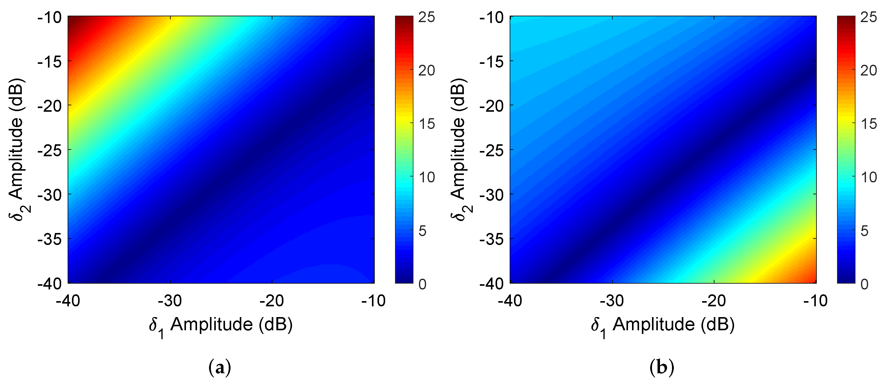
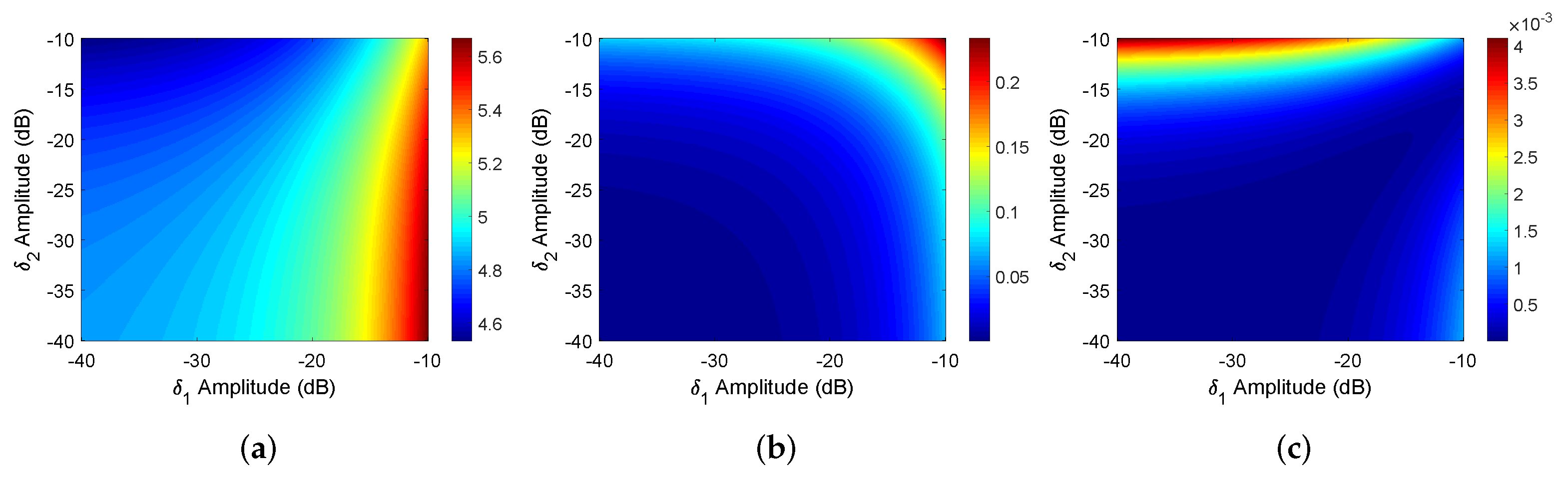
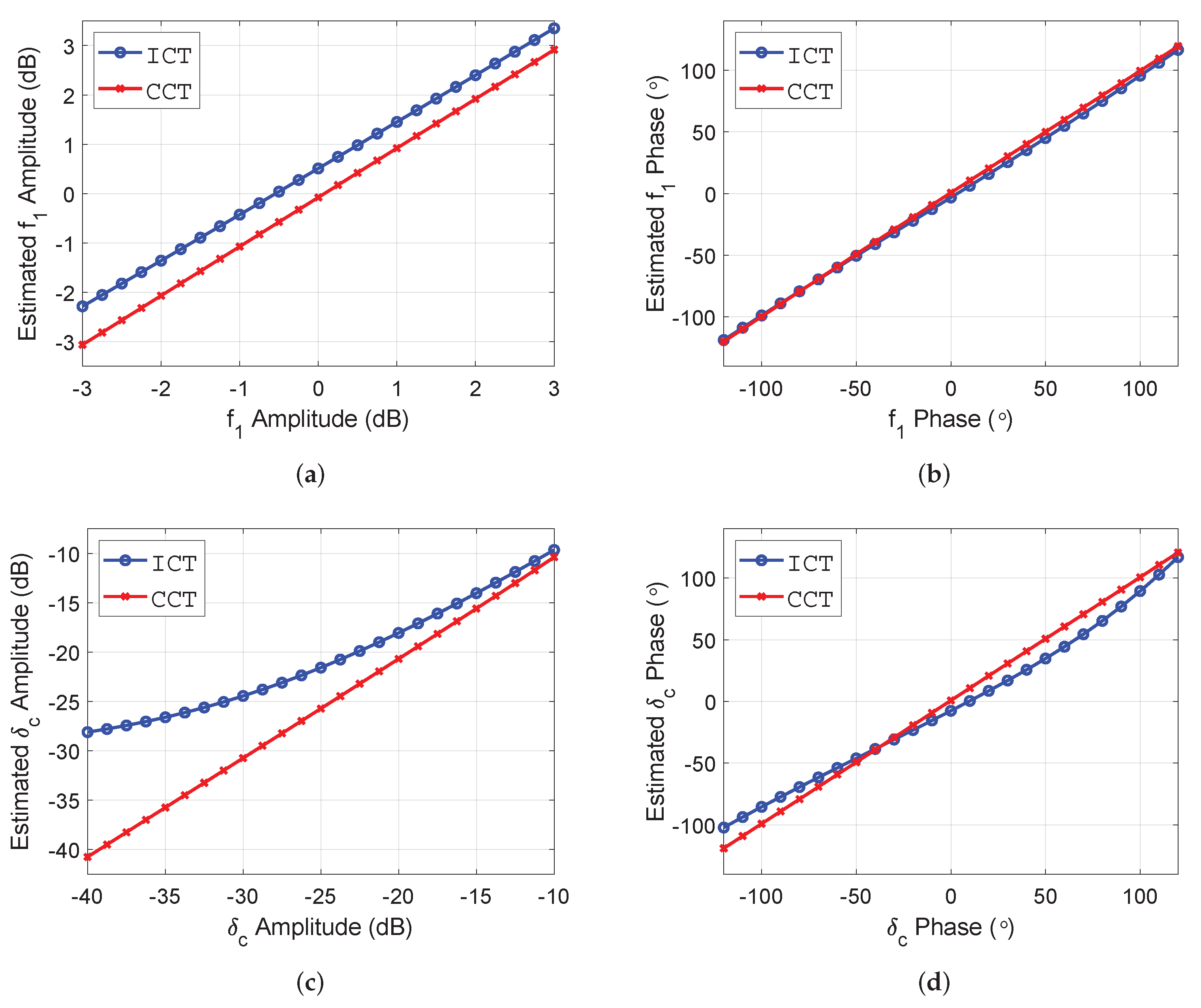
4.1. The Effect of Crosstalk on Calibration Schemes

We simulated the estimation error when each distortion parameter changes with crosstalk under the T2D calibrator configuration. The amplitude of δ 1 and δ 2 changes from 40 dB to 10 dB. The rotated dihedral calibrator in T2D is usually set to 22.5 or 45 , and the simulation results of these two settings are almost the same. Therefore, in the following content, we only give the result of 22.5 rotated dihedral. In the simulation, the channel imbalance is set to | f 1 | = 3   dB , arg { f 1 } = 30 . The transmission crosstalk is set to | δ c | = 20 dB , arg { δ c } = 40 Three amplitude coefficients are set to 0 dB, 1.5 dB and −1.5 dB, respectively. The phases coefficients are set to 36 , 51 , and 75 . The phases of δ 1 and δ 2 are set to 10 and 50 respectively.
Figure 2 shows the variation of channel imbalance and transmission crosstalk estimation error with received crosstalk. The horizontal axis represents δ 1 , and the vertical axis represents δ 2 . The first row and the second row are channel imbalance and transmission crosstalk estimation error, respectively. The first column is the amplitude estimation error, and the second column is the phase estimation error. The lower left corners of all subgraphs are displayed in blue, which means that when the crosstalk level is relatively low, the estimation error of the polarimetric distortion parameter is small. As the crosstalk level gradually increases to −10 dB, the estimation accuracy of each parameter also decreases. In the given example, the maximum error of channel amplitude imbalance can reach 1 dB, and the phase imbalance can reach 10 . The effect of transmission crosstalk with crosstalk is obviously greater than the channel imbalance parameter, and the maximum amplitude error and phase error are about 5 dB and 30 . Since the transmission crosstalk itself is small, the relative error will fluctuate more. We use the transmission axial ratio to judge the estimation accuracy of the actual transmission state.
Figure 3 shows the estimated error of the transmission AR, which is directly calculated by the method in Appendix A based on the above transmission crosstalk. It can conclude that when the crosstalk level is low, the transmission axial ratio estimation error is also at a relatively low level. When the receiving crosstalk increases, the transmission axial ratio estimation error also gradually increases to 1 dB. Figure 4 shows the estimated error of the ICT scheme for amplitude and phase coefficients emphasized in this paper. The first column is the amplitude coefficient estimation error, and the second column is the phase coefficient estimation error.
The characteristics of all parameters in Figure 4 are similar to the above. As the crosstalk level increases, the estimation error will increase to varying degrees. It is worth noting that coefficient estimation errors have different sensitivity to δ 1 and δ 2 . For example, the estimation error of A 1 is more sensitive to changes in δ 2 , while A 2 and A 3 are more sensitive to changes in δ 1 . This may be related to the optimization process and the sensitivity of the parameters in the transmission model. Combining the above results, a rough conclusion can be drawn. When the crosstalk level is better than −30 dB, the ICT scheme can obtain relatively accurate estimates of each distortion parameter.
To obtain more accurate and quantitative conclusions, the effect of receiving the crosstalk phase also needs to be taken into the consideration. We simulated the maximum estimation error of each distortion parameter under different receiving crosstalk levels (other parameters are kept the same as above). The simulation results are given in Table 1. For example, the first number 0.10 indicates that the maximum estimation error of f 1 amplitude is 0.10 dB when δ 1 and δ 2 are not better than −40 dB. Combined with the data in the table, if the approximate crosstalk level of the SAR antenna is known, the accuracy of the ICT calibration scheme can be estimated by looking up the table.
From Table 1, the estimation accuracy of the polarimetric distortion parameter shows a downward trend with the increase of crosstalk. When the crosstalk level is better than −30 dB, the estimated error of the amplitude and phase of the channel imbalance obtained by the ICT scheme is better than 0.31 dB and 2.11 . The estimated errors of the amplitude and phase of δ c are lower than 1.42 dB and 10.76 , and the corresponding AR estimation error does not exceed 0.31 dB. The estimation accuracy of amplitude and phase coefficients is lower than 0.30 dB and 1.84 respectively. It is worth noting that only the maximum estimated error is given in the table, which represents an upper limit. In most cases, the actual estimated error will be lower than this value. Therefore, these error ranges are acceptable.
The effect of the receiving crosstalk level on the ICT scheme is quantitatively analyzed above, and the corresponding application scope recommendations are provided. Below, we analyze the estimation accuracy of the CCT scheme for receiving crosstalk. The estimation accuracy of the CCT scheme under different receiving crosstalk levels is analyzed through simulation, and the estimated errors (differences between estimated and true values) are shown in Figure 5. The specific simulation parameters are consistent with the previous settings.
The results show that the CCT scheme cannot always accurately estimate the crosstalk value. When the level of the two crosstalks is comparable, the estimation error will be relatively small. Therefore, the constraint condition for using the CCT algorithm to estimate a more accurate crosstalk value is that the two crosstalk levels of the receiving channel should be close. Another reason for the large maximum estimation error of the receiving crosstalk in the above simulation results may be due to its low level, which is similar to the previous transmission crosstalk. Although the estimation error of this parameter is large, it may still be close to the real situation. Thus, to demonstrate the effectiveness of the CCT scheme, we further give the worst estimation accuracy of the CCT scheme for other distortion parameters under a given crosstalk level. Table 2 gives the specific results.
Overall, the upper limit of the estimated error obtained by CCT scheme is lower than that of ICT scheme under the same crosstalk level. However, it is worth noting that when the crosstalk is lower than −20 dB, the difference of the amplitude and phase coefficient estimation error between the two schemes is small, and the CCT scheme performs slightly better than the ICT scheme. The main difference between the two is the estimation of channel imbalance and transmission crosstalk. For example, when the crosstalk is −30 dB, the estimation error of the amplitude and phase of the channel imbalance in the CCT scheme is better than 0.09 dB and 0.56 , which is significantly higher than the ICT scheme by 0.22 dB and 1.55 , respectively. In addition, Table 2 also indicates that the maximum estimation error of the channel imbalance and transmission crosstalk of the CCT scheme with crosstalk level at −20 dB is similar to the case of the ICT scheme of crosstalk level at −30 dB. This proves that the CCT scheme relaxes the constraints on crosstalk compared to the ICT scheme.
In addition to the above analysis, we also discussed the rationality of using the estimator to correct the measured scattering vector when there is a certain error in the crosstalk estimation. Referring to the definition of similarity parameters [33], the following evaluation indicators are introduced.
γ = 20 log 1 3 i = 1 3 ( M i Correct ) H · M i True M i Correct 2 · M i True 2
M i True represents the theoretical scattering vector without receiving distortion (including only transmission distortion), and M i Correct represents the measured scattering vector after correction according to the estimated receiving distortion parameters.
M i True = [ S ] · E t
M i Correct = [ R ^ ] 1 M i · e j ϕ ^ i / A ^ i
γ is positive and characterizes the dissimilarity between M i True and M i Correct . γ = 0 dB indicates the two vectors are exactly the same. When γ is close to 0 dB, it means that the two vectors are similar, which also shows that it is reasonable to use the estimated distortion parameters for correction. Since this paper only corrects the distortion of the receiving channel, the theoretical measured vector used as a comparative standard still contains the influence of transmission crosstalk. The reason the theoretical measured vector containing only transmission crosstalk is used as the comparison standard is that this paper only considers the correction of the error of the receiving channel. As for the transmission distortion, it cannot be corrected based on the measured scattering vector [18].
Figure 6 shows the dissimilarity parameters between the corrected vector and the real vector before and after correction using ICT and CCT estimation parameters. The result shows that the original received vector is quite different from the actual received vector, and the approximate dissimilarity level is about 5 dB. After correction using the ICT scheme, the difference can be reduced to about 0.05 dB when the crosstalk is low. After correction using the CCT scheme, the dissimilarity value can be reduced to about 0.001 dB when the crosstalk level is low, or the crosstalk level is similar. This proves that the two schemes can perfectly correct the measured scattering vector even though the crosstalk is ignored, or the crosstalk estimation accuracy is not high. This also confirms that the crosstalk estimation accuracy has a limited effect on the final corrected vector. Therefore, if the accuracy of the measured scattering vector correction is used as the criterion, the accuracy assessment of the calibration scheme should mainly focus on the channel imbalance parameters and the transmission crosstalk.

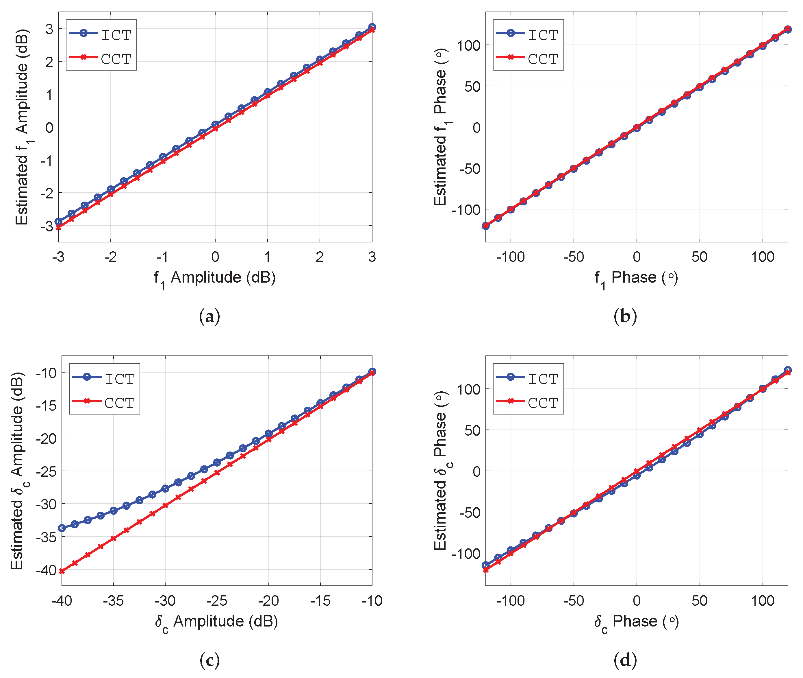
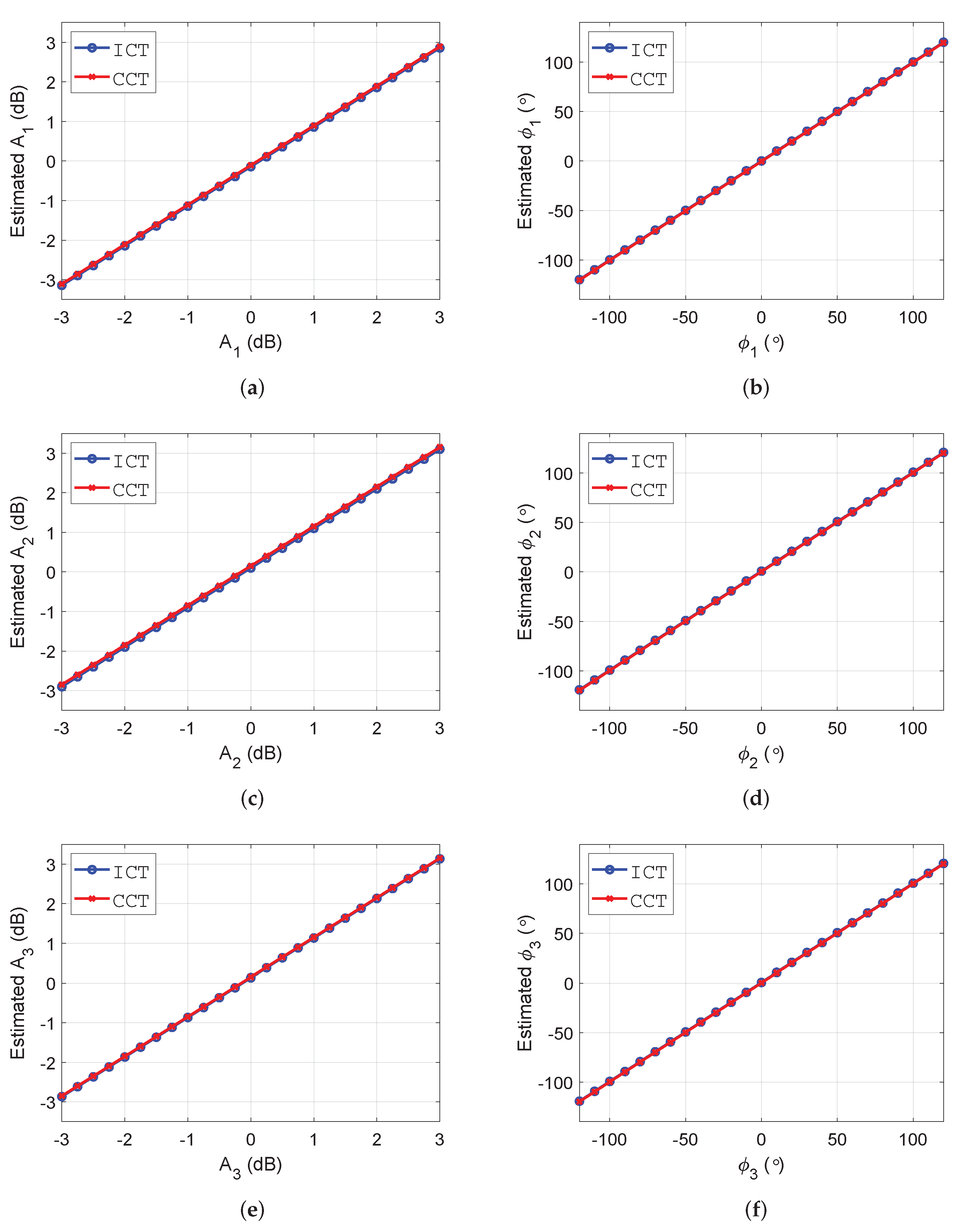
4.2. Estimation Accuracy of Distortion Parameters

In the following content, the distortion parameter estimation accuracy of the two calibration schemes is analyzed. To demonstrate the robustness of the calibration schemes, δ 1 and δ 2 are set to be relatively different. The amplitudes of δ 1 and δ 2 are set to −35 dB and −30 dB, and the phases are set to 10 and 50 , respectively. Other distortion parameters are set to be consistent with the above. Figure 7 shows the estimated channel imbalance and transmission crosstalk of the ICT and CCT schemes. Among them, the amplitude imbalance varies from −3 dB to 3 dB, and the transmission crosstalk amplitude varies from −40 dB to −10 dB. The range of phase imbalance and transmission crosstalk phase change is from 120 to 120 .
The results demonstrate that the estimation accuracy of the CCT scheme is generally higher than that of the ICT scheme. The ICT scheme can only achieve comparable performance to the CCT scheme when estimating the phase imbalance. For the amplitude imbalance, the estimated value obtained by the two schemes will slightly deviate from the true value by 0.1 dB to 0.2 dB. When estimating the transmission crosstalk amplitude, as its amplitude increases, the estimation error obtained by the ICT scheme will gradually decrease. One possible reason for this is that when the crosstalk is low, it is more sensitive to various error factors. For the transmission crosstalk phase, the estimated value of the ICT scheme slightly deviates from the true value of 5 .
Figure 8 further shows the amplitude and phase coefficient estimation of ICT and CCT calibration schemes. The three rows in the figure correspond to trihedral, dihedral, and 22.5 rotated dihedral, respectively. The first column is the amplitude coefficients error, and the second column is the phase coefficients error. The results suggest that both schemes can accurately estimate the actual coefficient values. The estimated error level of the actual amplitude coefficients is roughly 0.1 dB to 0.2 dB, and the phase coefficient estimation error is less than 1 . This also proves the correctness of the idea of “optimizing while compensating” in the calibration scheme. The above results prove that the proposed schemes can indeed reduce the requirements of polarimetric calibration for the radiometric calibration accuracy (e.g., accuracy of antenna pattern correction). Thus, the impact of radiometric calibration error on polarimetric calibration is reduced.
The above example is the error estimation situation when the crosstalk level is low. Next, we further demonstrate a case where the crosstalk level is relatively high ( | δ 1 | = 20 dB , | δ 2 | = 25 dB ), to observe the estimation error of channel imbalance and transmission crosstalk in this case. Figure 9 shows the estimated value of the corresponding channel imbalance parameter and transmission crosstalk. The characteristics shown in the figure are consistent with the case of low crosstalk. The overall estimation accuracy of the CCT scheme for each distortion parameter is still higher than that of the ICT scheme. In addition, the estimated characteristics of each specific distortion parameter are the same as in the low-crosstalk case for the ICT scheme. The only difference is that the estimation error is further increased. The estimation error of the amplitude imbalance between channels deteriorates to about 0.4 dB–0.8 dB. The maximum estimation error of transmission crosstalk has deteriorated from the original 7 dB to 12 dB. It is especially worth noting that after the crosstalk level increases, certain errors also occur when using the ICT scheme to estimate the phase imbalance. This also proves that it is not suitable to use the ICT scheme for calibration when the crosstalk level is relatively high.

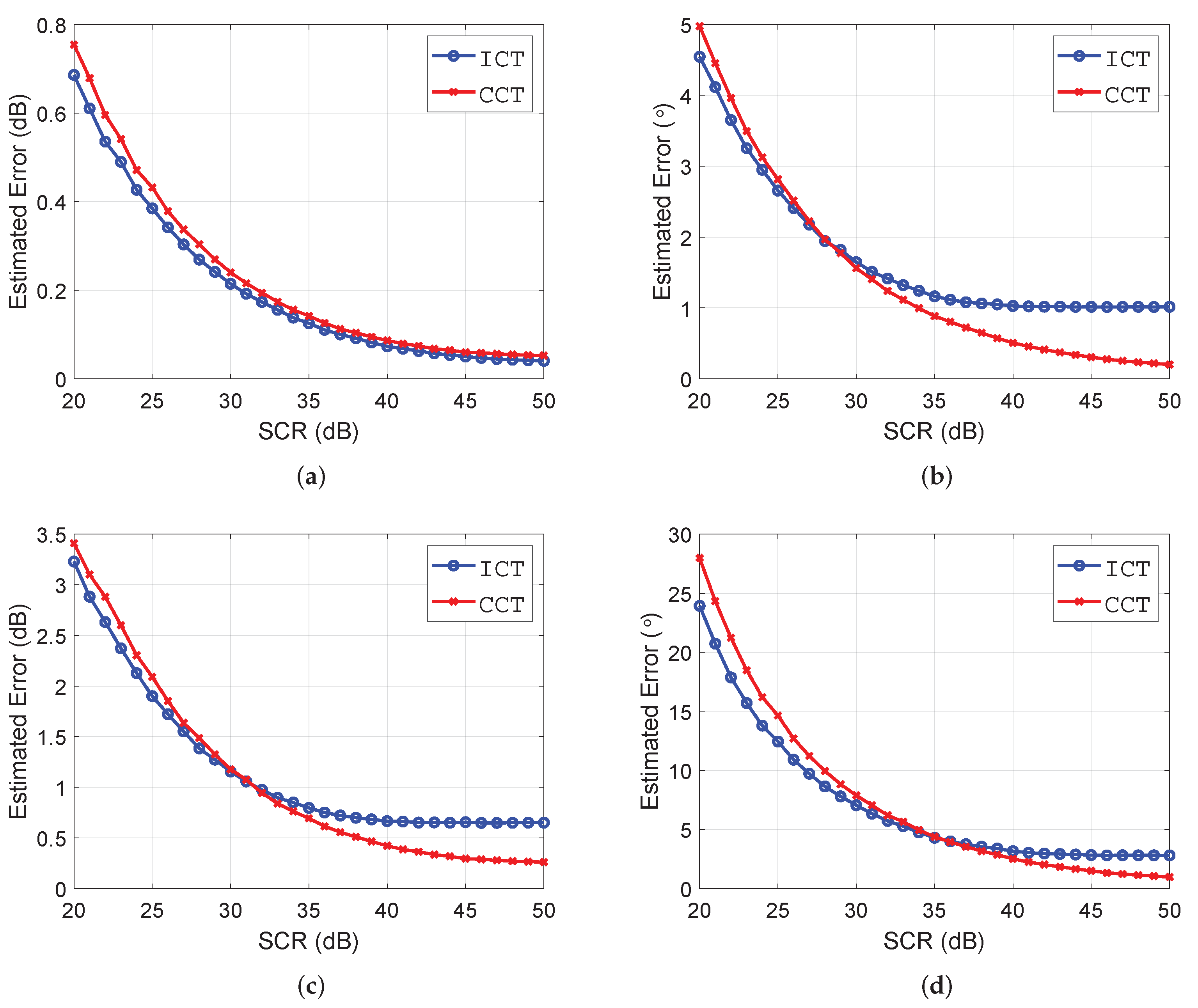
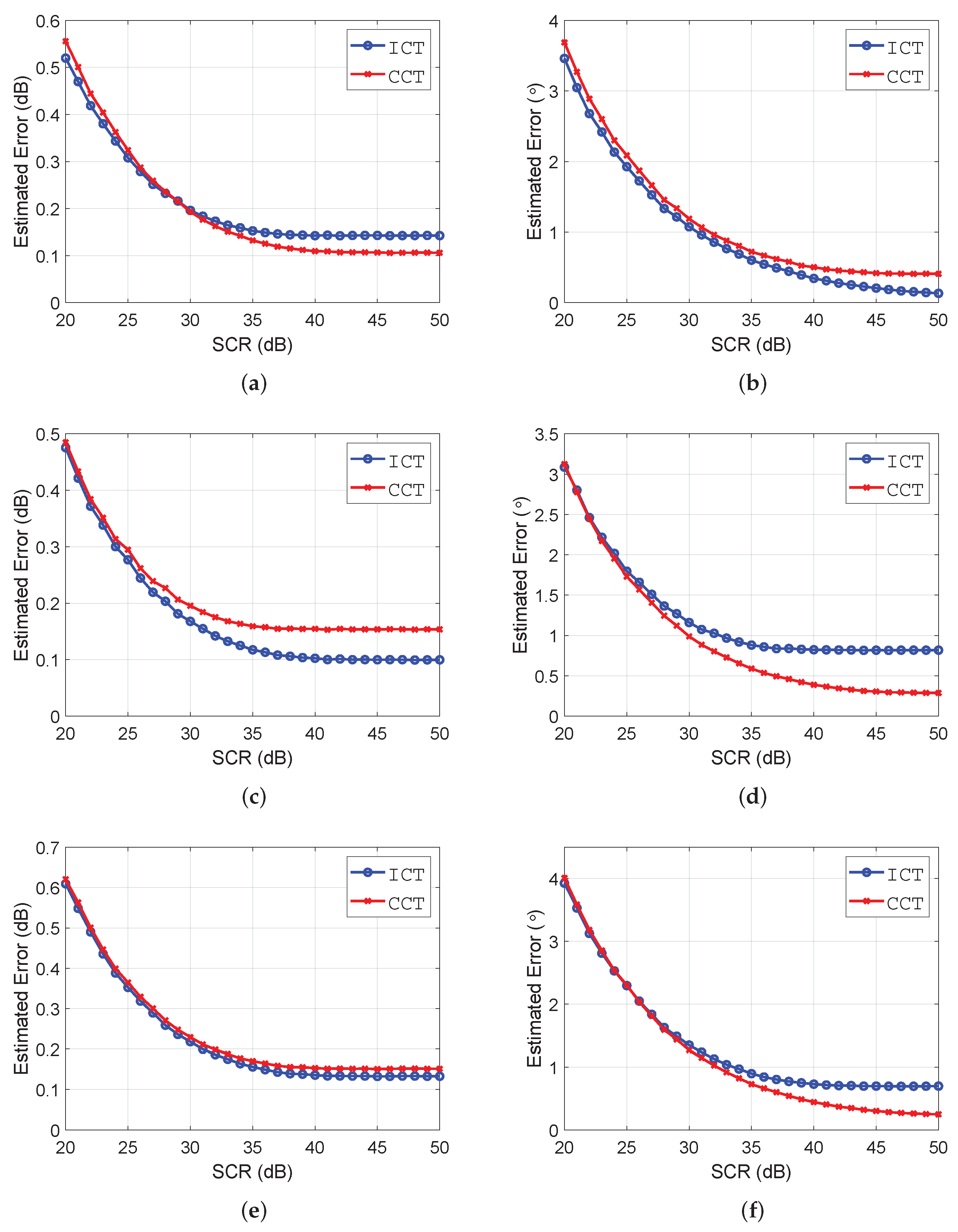
4.3. Effects of Clutter on Calibration Accuracy

Previous discussions are all noise-free cases. However, when extracting CR information in the actual calibration process, this will be affected by a certain level of clutter. Therefore, it is necessary to analyze the impact of different signal-to-clutter ratios (SCR) on the calibration results. The estimation error of each distortion parameter is analyzed through simulation when SCR changes between 20 dB and 50 dB (the settings of the other distortion parameters are consistent with the above case). In the experiment, it is assumed that the clutter satisfies the Gaussian distribution, and 10,000 Monte Carlo simulations are performed.
Figure 10 shows the estimation error of channel imbalance and transmission crosstalk under different SCR. Among them, the first row is channel imbalance, and the second row is transmission crosstalk. The first and second columns are the amplitude and phase errors, respectively. Figure 11 shows the estimated error of the amplitude and phase coefficients under different SCR. The three rows correspond to the trihedral, the dihedral, and 22.5 rotated dihedral, respectively. The first column is the amplitude coefficient estimation error, and the second column is the phase coefficient estimation error.
The results demonstrate that the estimation error of each distortion parameter will decrease with the increase of SCR. When the SCR is greater than 40 dB, the clutter has little effect on the final error estimation accuracy. It can be considered that the estimated value in this case is close to the estimated value in the ideal case without clutter. For the amplitude imbalance, the estimation accuracy of the two schemes is better than 0.1 dB when the SCR is greater than 40 dB. For phase imbalance and transmission crosstalk, when SCR is low, the estimation error of the ICT scheme is slightly better than that of the CCT scheme. When SCR is greater than 35 dB, the CCT scheme can obtain a higher estimation accuracy than ICT. When SCR is 50 dB, the estimation accuracy of the CCT scheme is better than 0.25 , 0.25 dB, and 2 , respectively. Under the same conditions, the estimation accuracy of the ICT scheme is relatively low, and the estimation error is roughly 1 , 0.7 dB, and 3 .

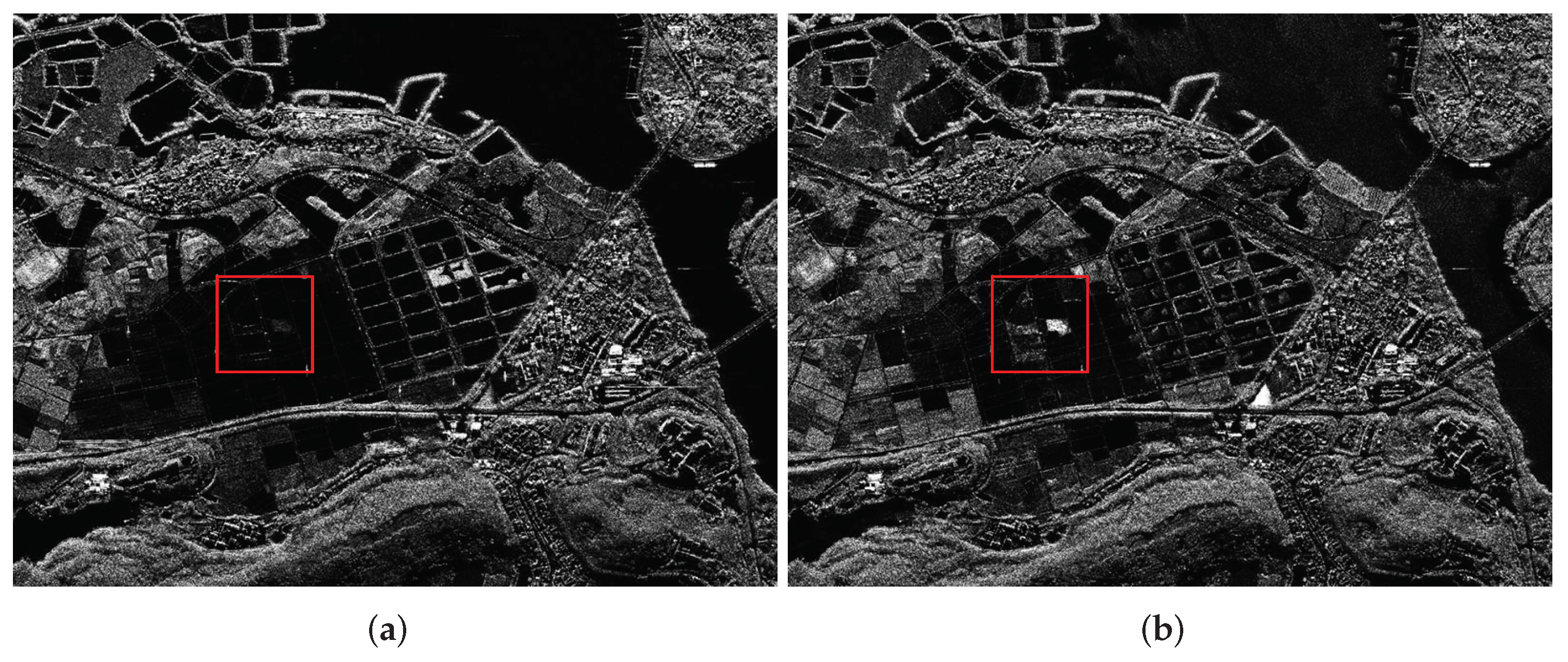
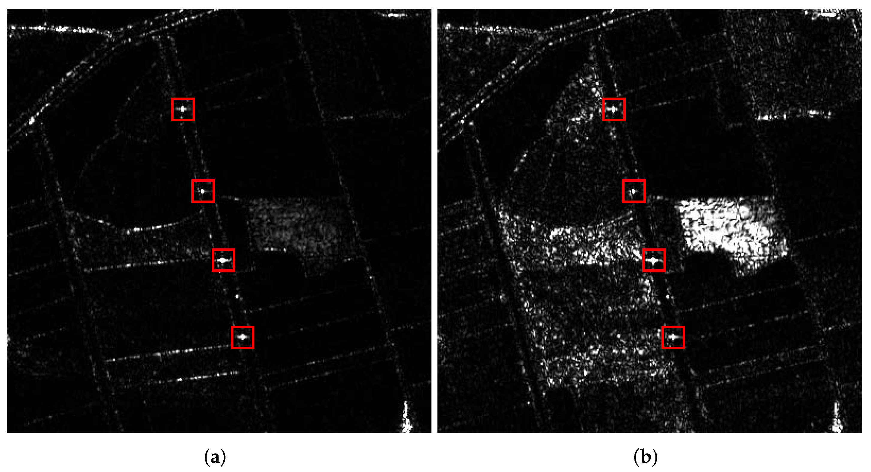
4.4. Results of AIRCAS L-Band Airborne SAR Data

In February 2021, the Aerospace Information Research Institute, Chinese Academy of Sciences (AIRCAS) carried out an L-band airborne hybrid quad-polarimetric SAR flight experiment in Boao, Hainan province, China. The experimental system alternately emits right-handed (R) and left-handed (L) circularly polarized electromagnetic waves, simultaneously using horizontal (H) and vertical (V) linearly polarized antennas for receiving single-look complex data of four polarimetric channels, HR, VR, HL, and VL. Many hybrid quad-polarimetric data are acquired in this experiment, which can provide data support for analyzing the characteristics of different targets under hybrid polarimetric basis or circularly polarimetric basis (synthesized from the original data).
Since the hybrid quad-polarimetric data are acquired in this experiment, we can extract the HR and VR channels to form the HCP data. There is only a difference in swath width between the extracted data and the data directly acquired by the real HCP system. Therefore, the data can be regarded as real HCP data and used for subsequent calibration analysis.
Figure 12 presents the intensity image of the extracted HCP data. The scene includes features such as ocean, farmland, and forest. Four CRs—two trihedral, one dihedral—and one 22.5 rotated dihedral, are deployed in the farmland. The layout position of the CRs is marked with a red box in Figure 12. Figure 13 shows an enlarged view of the calibration field, in which the red boxes mark the position of each CR. From top to bottom, they are trihedral, 22.5 rotated dihedral, dihedral, and trihedral.
There are two trihedral CRs in the scene and each trihedral can be combined with two dihedral CRs to form the T2D group required for calibration. Therefore, there are actually two T2D groups in the scene that can be used for calibration. We denote the CR group containing the top trihedral as T2D 1 , and the CR group containing the bottom trihedral as T2D 2 . After extracting the measured scattering vectors of the four CRs from the image, the ICT scheme and the CCT scheme are employed for calibration.
Table 3 gives the results of the distortion parameters calibrated using the above two sets of T2D calibrators. For the same calibration scheme, the results obtained by two different CR groups are similar. However, the distortion parameter values obtained by the ICT and CCT schemes are slightly different. It can be seen from the calibration results that although we have done antenna pattern correction, the amplitude coefficient deviation between the three CRs obtained by the two calibration schemes is up to 2 dB, and the difference between the phase coefficients is even greater. This also demonstrates that when using CRs for HCP calibration, the impact of the inconsistency of the amplitude and phase coefficients between the measured scattering vectors need to be additionally considered.
The SCR of four CRs in the image are all greater than 40 dB through calculation. Therefore, the distortion parameters obtained using the CCT scheme will have theoretically higher accuracy than the ICT scheme. Before the flight experiment, the researchers tested the transmission AR of the system in a microwave anechoic chamber, which is about 2 dB. This is very close to the transmission AR estimated by the CCT scheme, which also shows the effectiveness of the scheme.

5. Discussion

Aiming to solve the problem of inconsistency between the amplitude/phase coefficients of the measured scattering vectors for CRs during HCP calibration, this paper proposes two calibration schemes based on optimization algorithms. In the process of estimating the distortion parameters, we adopted the idea of “optimizing while compensating”. The word “compensating” has three meanings. Two meanings have been pointed out in the previous content, namely the compensation of the amplitude coefficients and the receiving error matrix to eliminate the influence of the unbalanced echo intensity between different CRs, and the unbalanced signal intensity between the H and V receiving channels. In addition, there is also compensation for phase coefficients. In the optimization objective function (5), the modulus difference between the measured scattering vector M i and the theoretical error vector E r , i is directly evaluated. If there is only a phase difference between the two, i.e., M i = e j ϕ E r , i , the difference between the two should be 0, in theory. However, when using (5), the difference will be very large. Therefore, it is necessary to eliminate this problem by individually compensating the phase coefficient.
Although two calibration schemes are proposed in the paper, they each have their own applicable conditions, and there is no one scheme that can always perform better than the other. The ICT scheme ignores the influence of crosstalk, which is destined to only adapt to low-crosstalk conditions where the crosstalk level is better than −30 dB. For the CCT scheme, the parameter estimation process is actually an optimized solution to an under-determined problem, and naturally, there are certain requirements for the characteristics of the distortion parameters. The simulation experiment shows that the CCT scheme can only accurately estimate the crosstalk when receiving crosstalk are close. If it is necessary to accurately estimate other polarimetric distortion parameters, the received receiving level is required to be lower than −20 dB. Although the CCT scheme expands the applicable range of crosstalk level compared with the ICT scheme, Section 4 reveals that only when SCR is higher than 35 dB does the CCT scheme achieve higher estimation accuracy than the ICT scheme. Therefore, in the actual calibration process, the prior value of the system distortion parameter and the actual SCR conditions should be combined to select the applicable calibration scheme.
The influence of Faraday rotation is not considered in the calibration scheme proposed in this paper. However, for long-wavelength spaceborne SAR systems, this is one of the factors that must be considered in the calibration process. In fact, the two schemes proposed in this paper are still available when the Faraday rotation effect exists. Tan points out [34] that the transmitter error can also be characterized by an equivalent crosstalk parameter when Faraday rotation exists:
E t = [ Ω ] · E t = cos Ω sin Ω sin Ω cos Ω 1 j + δ c 1 j = e j Ω 1 j + δ c e j 2 Ω 1 j
Therefore, after considering the Faraday rotation effect, an additional phase related to the Faraday rotation angle is added to the original transmission crosstalk. For the receiving channel, the equivalent receiving error matrix after considering the Faraday rotation effect can be expressed by (13).
[ R ] = [ R ] · [ Ω ] = 1 δ 2 δ 1 f 1 cos Ω sin Ω sin Ω cos Ω = cos Ω δ 2 sin Ω δ 2 cos Ω + sin Ω δ 1 cos Ω f 1 sin Ω f 1 cos Ω + δ 1 sin Ω = ( cos Ω δ 2 sin Ω ) 1 δ 2 δ 1 f 1
Combining (12) and (13), we can conclude that the original system model is still valid after considering the Faraday rotation effect, but all the distortion parameters are modulated by the Faraday rotation angle Ω . In this case, if the above scheme is used for calibration, although the actual Faraday rotation angle cannot be estimated, the error of the receiving channel can still be compensated to obtain data without receiving distortion. Moreover, after the actual Ω is estimated using the Total Electron Content (TEC) [35], the original distortion parameters can be recovered.

6. Conclusions

This paper points out that there are inconsistencies between the amplitude and phase coefficients of different CR-measured scattering vectors and these inconsistencies will seriously affect the estimation accuracy of the calibration scheme for system distortion parameters. Therefore, this paper proposes two calibration schemes for simultaneously estimating traditional distortion parameters and amplitude and phase coefficients under cases of ignoring crosstalk (ICT) and considering crosstalk (CCT). The CCT scheme takes the error estimate of the ICT scheme as the initial value, and further iterative optimization solutions are carried out on this basis. Two calibration schemes have different applicable conditions. Based on simulation experiments, it is concluded that the worst-receiving crosstalk levels applicable to the ICT and the CCT scheme are −30 dB and −20 dB, respectively. The estimation accuracies of each distortion parameter under the two cases of low crosstalk and medium crosstalk are also analyzed through simulation, and the results show that the CCT scheme can achieve higher accuracy. However, the CCT calibration scheme can only exert excellent performance when SCR is higher than 35 dB. In addition, L-band airborne HCP SAR data in Hainan, China acquired by AIRCAS has been used to prove the effectiveness of the calibration scheme. Therefore, the method in this paper helps to promote the practical application of the HCP calibration scheme based on CRs.

Author Contributions

Conceptualization, W.H.; methodology, W.H.; software, W.H.; validation, W.H., Y.G. and X.L.; formal analysis, X.L. and R.W.; investigation, W.H. and Y.H.; resources, F.Z.; data curation, R.W.; writing—original draft preparation, W.H.; writing—review and editing, F.Z., X.L., Y.G., D.L. and R.W.; visualization, W.H.; supervision, F.Z., X.L., D.L. and R.W.; project administration, F.Z. and R.W.; funding acquisition, F.Z., X.L. and R.W. All authors have read and agreed to the published version of the manuscript.

Funding

This work was funded by the Beijing Municipal Natural Science Foundation (No. 4192065) and National Natural Science Foundation of China (No. 61901445).

Institutional Review Board Statement

Not applicable.

Informed Consent Statement

Not applicable.

Data Availability Statement

Data sharing not applicable.

Acknowledgments

The authors would like to thank the Department of Space Microwave Remote Sensing System, Aerospace Information Research Institute, Chinese Academy of Sciences for providing L-band hybrid polarimetric SAR data. The authors would also like to thank all colleagues who participated in this experiment. Special thanks to Chunle Wang for her help in revising the manuscript.

Conflicts of Interest

The authors declare no conflict of interest.

Appendix A. Calculate the Axial Ratio (AR) from Transmission Crosstalk δc

Based on electromagnetic theory, any polarized wave can be described by a polarization ellipse [36] and the actual emission electromagnetic waves E t in this paper can be expressed by
E t = cos θ sin θ sin θ cos θ cos χ j sin χ
where the absolute amplitude and phase terms are ignored. θ is the ellipse orientation angle, and χ is the ellipticity angle. The parameter χ describes the “circularity” of the emitted signal. χ = 45 indicates the emitted electromagnetic waves are perfectly circularly polarized and χ = 0 indicates the emitted electromagnetic waves are linearly polarized electromagnetic waves. Axial ratio (AR) [37] is an index that quantitatively describes the emission error.
AR = cot | χ |
To obtain AR, the ellipticity angle must be calculated first. Given the transmission crosstalk, the Jons vector of the actual emitted sinal E t is known. Rotate E t according to the following equation.
E t ( θ ) = E t H ( θ ) E t V ( θ ) = cos θ sin θ sin θ cos θ · E t
Find θ that when the phase difference between the H and V channels is 90 , that is arg { E t H ( θ ) E t V * ( θ ) } = ± 90 . Thus, θ ˜ = θ . The corresponding ellipticity angle can be obtained by
tan χ ˜ = min | E t V ( θ ˜ ) | | E t H ( θ ˜ ) | , | E t H ( θ ˜ ) | | E t V ( θ ˜ ) |

References

  1. Raney, R.K. Hybrid-polarity SAR architecture. IEEE Trans. Geosci. Remote Sens. 2007, 45, 3397–3404. [Google Scholar] [CrossRef] [Green Version]
  2. White, L.; Millard, K.; Banks, S.; Richardson, M.; Pasher, J.; Duffe, J. Moving to the RADARSAT Constellation Mission: Comparing Synthesized Compact Polarimetry and Dual Polarimetry Data with Fully Polarimetric RADARSAT-2 Data for Image Classification of Peatlands. Remote Sens. 2017, 9, 573. [Google Scholar] [CrossRef] [Green Version]
  3. Yin, J.; Yang, J. Framework for Reconstruction of Pseudo Quad Polarimetric Imagery from General Compact Polarimetry. Remote Sens. 2021, 13, 530. [Google Scholar] [CrossRef]
  4. Hou, W.; Zhao, F.; Liu, X.; Wang, R. General Two-Stage Model-Based Three-Component Hybrid Compact Polarimetric SAR Decomposition Method. IEEE J. Sel. Topics Appl. Earth Observ. Remote Sens. 2021, 14, 4647–4660. [Google Scholar] [CrossRef]
  5. Hou, W.; Zhao, F.; Liu, X.; Zhang, H.; Wang, R. A Unified Framework for Comparing the Classification Performance between Quad-, Compact-, and Dual-Polarimetric SARs. IEEE Trans. Geosci. Remote Sens. 2021, 60, 1–14. [Google Scholar] [CrossRef]
  6. Dabboor, M.; Geldsetzer, T. Towards sea ice classification using simulated RADARSAT Constellation Mission compact polarimetric SAR imagery. Remote Sens. Environ. 2014, 140, 189–195. [Google Scholar] [CrossRef]
  7. Ponnurangam, G.G.; Jagdhuber, T.; Hajnsek, I.; Rao, Y. Soil moisture estimation using hybrid polarimetric SAR data of RISAT-1. IEEE Trans. Geosci. Remote Sens. 2015, 54, 2033–2049. [Google Scholar] [CrossRef]
  8. Olthof, I.; Rainville, T. Evaluating Simulated RADARSAT Constellation Mission (RCM) Compact Polarimetry for Open-Water and Flooded-Vegetation Wetland Mapping. Remote Sens. 2020, 12, 1476. [Google Scholar] [CrossRef]
  9. Raney, R.K. Hybrid dual-polarization synthetic aperture radar. Remote Sens. 2019, 11, 1521. [Google Scholar] [CrossRef] [Green Version]
  10. Spudis, P.; Nozette, S.; Bussey, B.; Raney, K.; Winters, H.; Lichtenberg, C.L.; Marinelli, W.; Crusan, J.C.; Gates, M.M. Mini-SAR: An imaging radar experiment for the Chandrayaan-1 mission to the Moon. Curr. Sci. 2009, 96, 533–539. [Google Scholar]
  11. Vondrak, R.; Keller, J.; Chin, G.; Garvin, J. Lunar Reconnaissance Orbiter (LRO): Observations for lunar exploration and science. Space Sci. Rev. 2010, 150, 7–22. [Google Scholar] [CrossRef]
  12. Misra, T.; Rana, S.; Desai, N.; Dave, D.; Rajeevjyoti Arora, R.K.; Rao, C.; Bakori, B.; Neelakantan, R.; Vachchani, J. Synthetic aperture radar payload on-board RISAT-1: Configuration, technology and performance. Curr. Sci. 2013, 104, 446–461. [Google Scholar]
  13. Kankaku, Y.; Suzuki, S.; Osawa, Y. ALOS-2 mission and development status. In Proceedings of the 2013 IEEE International Geoscience and Remote Sensing Symposium—IGARSS, Melbourne, Australia, 21–26 July 2013; pp. 2396–2399. [Google Scholar]
  14. Thompson, A.A. Overview of the RADARSAT Constellation Mission. Can. J. Remote Sens. 2015, 41, 401–407. [Google Scholar] [CrossRef]
  15. Brisco, B.; Mahdianpari, M.; Mohammadimanesh, F. Hybrid Compact Polarimetric SAR for Environmental Monitoring with the RADARSAT Constellation Mission. Remote Sens. 2020, 12, 3283. [Google Scholar] [CrossRef]
  16. Jung, Y.T.; Park, S.E. Comparative Analysis of Polarimetric SAR Calibration Methods. Remote Sens. 2018, 10, 2060. [Google Scholar] [CrossRef] [Green Version]
  17. Freeman, A.; Dubois-Fernandez, P.; Truong-Loi, M.L. Compact Polarimetry at longer wavelengths-calibration. In Proceedings of the 7th European Conference on Synthetic Aperture Radar, Friedrichshafen, Germany, 2–5 June; pp. 1–4.
  18. Truong-Loï, M.L.; Dubois-Fernandez, P.; Pottier, E.; Freeman, A.; Souyris, J.C. Potentials of a compact polarimetric SAR system. In Proceedings of the 2010 IEEE International Geoscience and Remote Sensing Symposium—IGARSS, Honolulu, HI, USA, 25–30 July 2010; pp. 742–745. [Google Scholar]
  19. Babu, A.; Kumar, S.; Agrawal, S. Polarimetric calibration of RISAT-1 compact-pol data. IEEE J. Sel. Topics Appl. Earth Observ. Remote Sens. 2019, 12, 3731–3736. [Google Scholar] [CrossRef]
  20. Kumar, S.; Babu, A.; Agrawal, S.; Asopa, U.; Shukla, S.; Maiti, A. Polarimetric calibration of spaceborne and airborne multifrequency SAR data for scattering-based characterization of manmade and natural features. Adv. Space Res. 2021. [Google Scholar] [CrossRef]
  21. Chen, J.; Quegan, S. Calibration of spaceborne CTLR compact polarimetric low-frequency SAR using mixed radar calibrators. IEEE Trans. Geosci. Remote Sens. 2011, 49, 2712–2723. [Google Scholar] [CrossRef]
  22. Sabry, R. A tool for analysis and calibration of compact polarimetry SAR mode anomaly. IEEE Geosci. Remote Sens. Lett. 2018, 15, 424–428. [Google Scholar] [CrossRef]
  23. Touzi, R.; Shimada, M.; Motohka, T.; Nedelcu, S. Assessment of PALSAR-2 Compact Non-Circularity Using Amazonian Rainforests. IEEE Trans. Geosci. Remote Sens. 2020, 58, 7472–7482. [Google Scholar] [CrossRef]
  24. Tan, H.; Hong, J. Calibration of compact polarimetric SAR images using distributed targets and one corner reflector. IEEE Trans. Geosci. Remote Sens. 2016, 54, 4433–4444. [Google Scholar] [CrossRef]
  25. Freeman, A.; Alves, M.; Chapman, B.; Cruz, J.; Kim, Y.; Shaffer, S.; Sun, J.; Turner, E.; Sarabandi, K. SIR-C data quality and calibration results. IEEE Trans. Geosci. Remote Sens. 1995, 33, 848–857. [Google Scholar] [CrossRef]
  26. Ulander, L.M.H.; Hawkins, R.K.; Livingstone, C.E.; Lukowski, T.I. Absolute radiometric calibration of the CCRS SAR. IEEE Trans. Geosci. Remote Sens. 1991, 29, 922–933. [Google Scholar] [CrossRef]
  27. Bhiravarasu, S.S.; Chakraborty, T.; Putrevu, D.; Pandey, D.K.; Kumar, R. Chandrayaan-2 Dual-Frequency SAR (DFSAR): Performance Characterization and Initial Results. Planet. Sci. J. 2021, 2, 134. [Google Scholar] [CrossRef]
  28. Sharma, S.; Dadhich, G.; Rambhia, M.; Mathur, A.K.; Prajapati, R.; Patel, P.; Shukla, A. Radiometric calibration stability assessment for the RISAT-1 SAR sensor using a deployed point target array at the Desalpar site, Rann of Kutch, India. Int. J. Remote Sens. 2017, 38, 7242–7259. [Google Scholar] [CrossRef]
  29. Zhao, L.; Li, Y.; Zhang, Q.; Liu, J.; Yuan, X.; Chen, Q. Design and Verification of Image Quallity Indexes of GF-3 Satellite. Spacecr. Eng. 2017, 6, 18–23. [Google Scholar] [CrossRef]
  30. Whitt, M.; Ulaby, F.; Polatin, P.; Liepa, V. A general polarimetric radar calibration technique. IEEE Trans. Antennas Propag. 1991, 39, 62–67. [Google Scholar] [CrossRef]
  31. Roweis, S. Levenberg-Marquardt Optimization. Notes; University of Toronto: Toronto, ON, Canada, 1996. [Google Scholar]
  32. Ranganathan, A. The levenberg-marquardt algorithm. Tutor. LM Algorithm 2004, 11, 101–110. [Google Scholar]
  33. Yang, J.; Peng, Y.N.; Lin, S.M. Similarity between two scattering matrices. Electron. Lett. 2001, 37, 193–194. [Google Scholar] [CrossRef]
  34. Tan, H. Study on Methods of Calibration and Correction of Compact Polarimetric SAR. Ph.D. Thesis, University Chinese Academy of Sciences, Beijing, China, June 2016. [Google Scholar]
  35. Wright, P.A.; Quegan, S.; Wheadon, N.S.; Hall, C.D. Faraday rotation effects on L-band spaceborne SAR data. IEEE Trans. Geosci. Remote Sens. 2003, 41, 2735–2744. [Google Scholar] [CrossRef]
  36. Lee, J.S.; Pottier, E. Polarimetric Radar Imaging: From Basics to Applications; CRC Press: New York, NY, USA, 2017. [Google Scholar]
  37. Knittel, G. The polarization sphere as a graphical aid in determining the polarization of an antenna by amplitude measurements only. IEEE Trans. Antennas Propag. 1967, 15, 217–221. [Google Scholar] [CrossRef]
Figure 1. The impact on the estimation accuracy of channel imbalance parameters when the amplitude and phase coefficients of the CR-measured scattering vectors are inconsistent. The first and second row respectively represent the results when trihedral or dihedral is the “inconsistent” CR. (a,c) are estimation errors for amplitude imbalance (dB). (b,d) are estimation errors for phase imbalance ( ).
Remotesensing 14 00416 g001
Figure 2. The distortion parameter estimation error of the ICT scheme under different crosstalk levels. (a) amplitude imbalance (dB). (b) phase imbalance ( ). (c) amplitude of transmission crosstalk (dB). (d) phase of transmission crosstalk ( ).
Remotesensing 14 00416 g002
Figure 3. The estimation error of the ICT calibration scheme for the transmission axial ratio under different crosstalk levels.
Remotesensing 14 00416 g003
Figure 4. The amplitude and phase coefficients estimation error of the ICT calibration scheme under different crosstalk levels. The first column is the amplitude coefficient estimation error, and the second column is the phase coefficient estimation error. (a,b) are estimation errors of trihedral ( A 1 , ϕ 1 ). (c,d) are estimation errors of dihedral ( A 2 , ϕ 2 ). (e,f) are estimation errors of 22.5 rotated dihedral ( A 3 , ϕ 3 ).
Remotesensing 14 00416 g004
Figure 5. The estimated error of the received crosstalk using the CCT scheme under different received crosstalk distortion conditions. (a) estimated error of δ 1 . (b) estimated error of δ 2 .
Remotesensing 14 00416 g005
Figure 6. The dissimilarity between measured scattering vector and the theoretical receiving vector containing only transmission errors. (a) Original measured scattering vector. (b) Measured scattering vector corrected by ICT scheme. (c) Measured scattering vector corrected by CCT scheme.
Remotesensing 14 00416 g006
Figure 7. Simulation of distortion parameters estimation. (a) | f 1 | (dB). (b) arg { f 1 }   ( ) . (c) | δ c | (dB). (d) arg { δ c }   ( ) .
Remotesensing 14 00416 g007
Figure 8. Simulation of amplitude and phase coefficients estimation. (a) | A 1 | (dB). (b) ϕ 1   ( ) . (c) | A 2 | (dB). (d) ϕ 2   ( ) . (e) | A 3 | (dB). (f) ϕ 3   ( ) .
Remotesensing 14 00416 g008
Figure 9. Simulation of distortion parameters estimation when the crosstalk level is relatively high ( | δ 1 | = 20 dB , | δ 2 | = 25 dB ). (a) | f 1 | (dB). (b) arg { f 1 }   ( ) . (c) | δ c | (dB). (d) arg { δ c }   ( ) .
Remotesensing 14 00416 g009
Figure 10. Simulation of distortion parameters estimation error with different SCR. (a) | f 1 | (dB). (b) arg { f 1 }   ( ) . (c) | δ c | (dB). (d) arg { δ c }   ( ) .
Remotesensing 14 00416 g010
Figure 11. Simulation of distortion parameters estimation error with different SCR. (a) | A 1 | (dB). (b) ϕ 1   ( ) . (c) | A 2 | (dB). (d) ϕ 2   ( ) . (e) | A 3 | (dB). (f) ϕ 3   ( ) .
Remotesensing 14 00416 g011
Figure 12. Intensity image of L-band airborne HCP data in Boao, Hainan province, China. (a) HR image. (b) VR image.
Remotesensing 14 00416 g012
Figure 13. Enlarge intensity image of L-band airborne HCP data in Boao, Hainan province, China. (a) HR image. (b) VR image.
Remotesensing 14 00416 g013
Table 1. The maximum estimation error of the distortion parameters obtained using the ICT scheme under different crosstalk levels.
DistortionReceiving Crosstalk Level (dB)
Parameters−40−35−30−25−20−15−10
| f 1 | (dB)0.100.180.310.541.012.115.04
arg { f 1 }   ( ) 0.671.202.113.726.6211.9221.34
| δ c | (dB)0.490.851.422.735.8014.7736.30
arg { δ c } ( ) 3.386.0210.7619.5036.7175.57219.78
A 1 (dB)0.070.130.220.400.721.354.23
A 2 (dB)0.090.170.300.540.961.753.32
A 3 (dB)0.090.150.270.490.891.633.10
ϕ 1   ( ) 0.460.821.442.554.638.6917.27
ϕ 2   ( ) 0.581.031.843.265.7710.2018.01
ϕ 3   ( ) 0.510.911.612.844.998.7415.59
AR (dB)0.100.180.310.540.901.432.15
Table 2. The maximum estimation error of the distortion parameters obtained using the CCT scheme under different crosstalk levels.
DistortionReceiving Crosstalk Level (dB)
Parameters−40−35−30−25−20−15−10
| f 1 | (dB)0.030.050.090.170.320.661.51
arg { f 1 }   ( ) 0.180.320.561.021.953.878.78
| δ c | (dB)0.140.260.460.811.452.594.69
arg { δ c }   ( ) 0.891.582.804.998.8615.7327.75
A 1 (dB)0.060.110.200.370.671.252.44
A 2 (dB)0.080.150.270.490.891.653.18
A 3 (dB)0.080.150.260.480.871.603.07
ϕ 1   ( ) 0.400.721.282.294.127.5514.20
ϕ 2   ( ) 0.510.901.612.865.129.2116.88
ϕ 3   ( ) 0.490.871.552.764.938.8816.25
AR (dB)0.030.050.090.170.320.611.24
Table 3. Estimated distortion parameters of L-band HCP data using ICT and CCT schemes.
DistortionICTCCT
ParametersT2D 1 T2D 2 T2D 1 T2D 2
| f 1 | (dB)−0.40−0.44−0.43−0.54
arg { f 1 }   ( ) −7.13−6.740.170.19
| δ c | (dB)−21.92−22.27−18.69−18.70
arg { δ c }   ( ) 164.87162.11136.53136.50
A 1 (dB)19.7319.2019.7019.22
A 2 (dB)18.6818.7018.5318.59
A 3 (dB)17.6117.6317.7117.78
ϕ 1   ( ) 101.63185.7697.49181.84
ϕ 2   ( ) 141.47141.27137.66137.63
ϕ 3   ( ) −90.01−90.19−94.57−94.47
AR (dB)1.401.342.032.03
Publisher’s Note: MDPI stays neutral with regard to jurisdictional claims in published maps and institutional affiliations.

