1. Introduction
Remote sensing image segmentation is mainly used to identify and segment out ground objects in images. Therefore, semantic segmentation, as a basic vision task, has essential applications in remote sensing image segmentation. Deep learning has yielded great results in the direction of fully supervised semantic segmentation [
1,
2,
3]. However, training a fully supervised semantic segmentation model requires many densely labeled images, and segmentation in remote sensing images requires more labeled samples, and the labeling process is laborious.
To alleviate the need for dense pixel annotation, few-shot segmentation of remote sensing images is proposed. Few-shot segmentation aims to segment novel classes according to common features among base classes learned during the training phase. A better-performing few-shot segmentation of remote sensing images model should be able to adapt to novel classes by learning only a few annotated samples. Currently, the majority of few-shot learning approaches adhere to a meta-learning paradigm. Due to better flexibility and accuracy, metric-based meta-learning models are widely used in few-shot segmentation tasks.
A typical few-shot segmentation model treats non-target classes as the background in support images, leading to specific features being undermined. The features of latent classes in the background can be taken as a reference to discriminate between the foreground and background. To this end, mining latent novel classes can widen the gap between the background and foreground prototypes. Furthermore, similar and dissimilar categories might be misclassified in the category representation space. Our method use contrastive learning to decrease the distance between similar categories and increase the distance between different categories in the embedding space, hence improving the feature extractor’s accuracy for category representation.
We propose a few-shot segmentation of the remote sensing images model using a self-supervised background learner to overcome the problem of feature undermining and discriminator bias. Considering that there is also rich feature information in the background of the support set, the background learner learns from the unlabeled data to assist the meta-learner for further feature enhancement. In addition, to learn richer general features between categories, our model uses contrastive learning to make the category embedding space more uniformly distributed and to retain more feature information.
In summary, our contributions lie in these particular aspects:
We propose that when segmenting novel classes, the background learner can learn the latent classes and assist the feature extractor in obtaining information about other classes in the background. The background learner eliminates confusion between the target class and non-target class objects with different semantics in the query image, and improves segmentation accuracy.
We use contrast learning to refine the segmented edges by explicitly classifying query and background features in the embedding space.
This provides a more accurate segmentation model for the few-shot segmentation of remote sensing images. This addresses the costly problem of annotating images of new classes in remote sensing.
2. Related work
2.1. Few-Shot Learning
In many application scenarios, the models have a limited number of annotated samples to generalize well. Few-shot learning is proposed, to recognize the novel classes with a few samples by learning meta-knowledge among the different categories. Generally, few-shot learning is classified as being model-based [
4], metrics-based [
5], and optimization-based [
6,
7,
8]. Particularly, the Siamese network [
9] laid the foundations for later metrics-based model growth. Additionally, the matching network [
6] provides another idea for the development of non-parametric metrics learning. In the metrics learning framework, the prototype network [
7] leads the model to focus on the similarity between the support and query pairs while ignoring semantic features learning.
2.2. Few-Shot Segmentation of Remote Sensing Images
In semantic segmentation, approaches on the basis of few-learning can segment novel classes with only a few annotated images. Recent works can be divided into two categories using different focal points, i.e., a parameter matching-based method and a prototype-based method. In a breakthrough of few-shot segmentation, PANet [
10] introduced a prototype alignment method that provides highly representative prototypes for each semantic class and that segments query objects based on feature matching. Furtherly, segmentation that is based on deep learning methods relies on big data training [
11,
12], but remote sensing images are densely annotated and laborious to acquire. The studies in [
13,
14,
15,
16,
17] explore how to reduce the need for dense annotation from self-/semi-supervised learning and weakly supervised learning. Jiang et al. [
18] introduced a few-shot learning method for remote sensing image segmentation. However, few-shot learning is not maturely applied in remote sensing image segmentation.
2.3. Self-Supervised Learning
The influence of a fully supervised learning model will be considerably constrained for specific tasks, owing to a lack of data and labels. However, self-supervised learning can improve the feature extraction ability of the model when faced with a new field and task that lacks abundant labeled data. MoCo’s [
19] appearance triggered a surge in visual self-supervised learning. Then, one by one, SimCLR [
20], BYOL [
21], SwAV [
22], and other self-supervised learning algorithms were proposed. The model can learn features using self-supervised learning based on a pretext task [
23]. A pretext task, such as generating a pseudo-label using a superpixel method, can provide additional local information that is used for few-shot learning to compensate for the lack of annotated data. Self-supervised learning has been widely used for the task of few-shot segmentation. For example, SSL-ALPNet [
24] employs superpixel-based pseudo-label rather than manual annotation. MLC [
25] uses an offline annotation module to generate pseudo masks of unlabeled data as a pretext task. SSNet [
26] obtains supervised information in the background of the query set via super-pixel segmentation.
3. Problem Setting
Our model conducts training process on base classes with abundant annotated images, and then use the generalization ability to segment novel classes with few annotated images (). Our model extracts images containing base classes from train set , and images including the novel classes compose test set . The training set is constructed using image-mask pairs that have objects in , where i states the i-th image and represents the corresponding mask. The test set has the same construction as the training set. A few-shot segmentation training episode typically consists of a set of query images Q and a set of supporting images S with ground-truth masks. We require the additional set of images E in our few-shot segmentation setting. In detail, a training episode of few-shot segmentation is composed of n ways for every way to have k shots support samples, q query images, and e extra images.
4. Methods
4.1. Overview
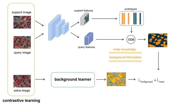
As previously mentioned, non-target classes in the images are simply treated as a background. To alleviate this issue, we consider the features of non-target classes that lead the feature extractor to learn features in the background. In addition, we apply contrastive learning to obtain a more accurate discriminator. Noteworthly, the meta-learner use fully supervised learning and the background learner use self-supervised learning. These two branches jointly supervise the feature extractor; hence, we define our model as semi-supervised learning.
Our framework. We designed a few-shot segmentation framework that learns meta-knowledge via training on supporting-query pairs, and that mines the latent novel classes in the contexts via self-supervised learning. With the auxiliary supervision named background learner, our method can learn semantic features in the background that help discriminate the support classes in the complicated scene. The model (
Figure 1) conducts semantic segmentation by first sending support and query images to an encoder that extracts features. Then, the support prototypes are computed from the prototype generation module that contains masked average pooling. The background learner trains the model with extra images to mine latent novel classes, as introduced in
Section 4.2. To learn richer general features between categories, our model employs contrastive learning via infoNCE loss, as described in
Section 4.3. Support and query prototypes from the meta learner are used as positive samples, whereas latent category prototypes from the background learner are kept as negative samples in the memory bank.
In this work, we added self-supervised learning from additional unlabeled images to learn the image background features. In the background learner, we added extra images into an encoder–decoder to obtain prediction maps where the encoder is shared with the characteristics extractor of the supporting and query images. Training with the additional branch, we calculated the segmentation loss
as follows:
where
represents the ground truth segmentation loss of the query image,
denotes the extra images segmentation loss, and
is the contrastive loss. The settings of hyperparameters
and
are analyzed in detail in
Section 6.2.5.
4.2. Background Learner
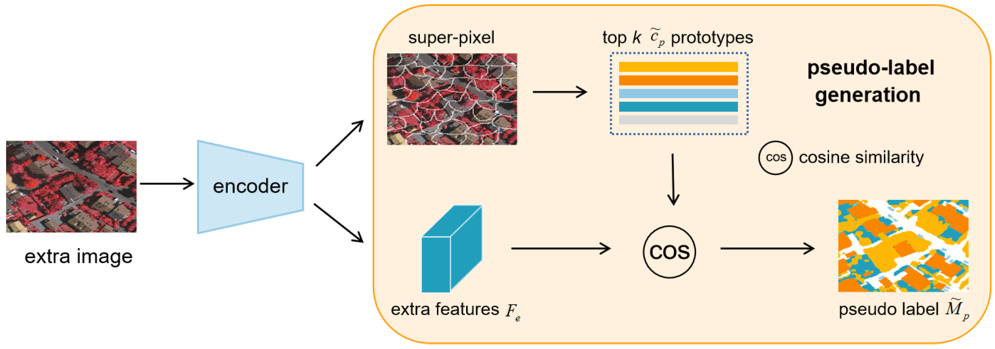
4.2.1. Pseudo-Label Generation
A self-supervised pretext task attempts to make greater use of background pixel information. Pseudo-label generation utilizes super-pixel segmentation to segment unlabeled data (
Figure 2). We chose SLIC as the method for superpixel generation. The SLIC method generates superpixels via iterative clustering. In detail, we set the compactness to 10 and n_segments to 100, and selected the five superpixels with the highest class activation values from the final
k generated superpixels as the background in potential classes. For the number of potential classes selected, we set
k to 5. In
Section 6.2.5, we demonstrate a comparison experiment for the hyperparameter k taking values.
The pseudo-label generation denotes each super-pixel as a pseudo-class
and generates the corresponding binary mask
. The class activation score
of each pseudo-class
is calculated by the average of the extracted extra feature
:
The five classes with the highest activation scores in the pseudo-classes were selected as the most likely latent novel classes in the background. The corresponding binary mask is denoted as .
4.2.2. Loss Function
The model optimizes the parameters by reducing the value of the loss function. The model applies a cross-entropy loss function in the background learner to supervise the training of our model. In the background learner branch, since our model defines the number of pseudo-classes to be five, the background learner uses a multi-category cross-entropy loss. We define
as the multi-category cross-entropy loss between the pseudo-class mask
and predicted extra mask
by:
where
is the height and width of feature maps,
represents the generated pseudo-class label, and
represents the predicted background feature mask.
4.3. Contrastive Representation Learning
Contrastive learning allows the model to learn similarities and differences between feature points to learn general features between categories. In the vector representation space, contrastive learning enables the model to bring positive samples closer to the anchor samples and negative samples further away.
Contrastive learning is more effective when there are enough negative samples; however, standard few-shot learning frameworks may relate to less negative samples. According to this question, we introduce extra unlabeled images as negative samples (
Figure 3). On the one hand, these extra images supervise the feature extractor in mining background information, and on the other hand, they can be utilized as negative examples in contrastive learning to supervise the model in learning general features between images.
To increase the negative samples set, we employ a memory bank to store negative samples, as inspired by SimCLR [
20]. k negative samples are stored in the memory bank, represented as
. The positive samples generated by query image encoding are denoted as
, while the negative samples generated by supporting image encoding are denoted as
, forming the space of all samples for the contrastive learning.
Positive samples are the support and query prototypes encoded from the support and query images, while negative samples are the potential background classes obtained from the background learner branch. Clustering between similar prototypes is strengthened by increasing the distance between the positive and negative samples using infoNCE loss [
19]:
where
denotes the loss between the positive and negative samples in contrastive learning.
represents the temperature coefficient; we set
, based on broad experiments.
is the distance measure function between the positive and negative samples; we chose the cosine similarity function as the measure function in this paper:
5. Experiments
5.1. Dataset and Metrics
PASCAL- and COCO-. The performance of our model is evaluated on two datasets, i.e., PASCAL-
and COCO-
. The PASCAL-
dataset has 20 classes, consisting of PASCAL VOC 2012 [
27] and augmented SBD [
28]. The COCO-
dataset contains 80 categories. In the few-shot segmentation task, the classes of both the datasets are divided into four folds; three folds are used for training, and the fourth fold is used for assessment.
Remote sensing dataset. We ran trials using the Vaihingen dataset and the Zurich Summer dataset to assess the effectiveness of our model for remote sensing. The Vaihingen dataset was provided by the International Society for Photogrammetry and Remote Sensing (ISPRS), which collected data from high-resolution aerial images of Vaihingen, with each image labeled with six classes. The Zurich Summer dataset consists of 20 photos, including eight classes. The Zurich dataset can reflect real-world conditions well, which helps with evaluating the performance of the segmentation models in remote sensing. Details of these two remote sensing datasets are shown in the (
Table 1).
Baseline and metrics. PANet was used as the baseline model, because our model is based on metric learning. Following previous methods, the mean Intersection-over-Union (mIoU) is adopted for evaluating the model performance. On in-domain and cross-domain transfer, the remote sensing image segmentation performance is assessed using the F1 score of each class, and the overall accuracy.
5.2. Implementation and Training Details
Network structure. To prove the effectiveness of our approach, ResNet-50 and ResNet-101 were separately applied to be the feature extractor. The last level of the ResNet is deleted for improved generalization, and the last ReLU is replaced by cosine similarity [
10]. As for the auxiliary semantic branch for learning background features, a lightweight decoder is introduced behind the encoder shared with the meta-learner. The decoder consists of three convolution layers, and all except the final convolution are followed by batch normalization and ReLU. ImageNet pre-trained ResNet parameters are used for initialization, as in previous approaches.
Implementation details. In particular, on PASCAL- and COCO-, all episodes are developed with a support-query pair, and an additional image that supervises the model learning background features in the training phase. To train the model, we used the SGD optimizer with a learning rate of 5 that decays by 0.1 every 10,000 iterations, and a momentum of 0.9. To obtain improved model parameters, the SGD backpropagation approach continually modifies the model parameters over 3000 iterations. The training image and mask pairs were cropped to (417,417) and enhanced through random horizontal flipping. Specifically, our model stores the negative samples in a memory bank where a dictionary is developed to store and update the embedding of negative samples. The system of this experiment was Ubuntu 16.04, and the processor was Intel Xeon Silver 4210R. The graphics processor (GPU) was the GeForce RTX 3090 GPU with 1 TB memory.
6. Discussion
6.1. Comparison with the State-of-the-Art
Extensive experiments were conducted to evaluate the model performance on PASCAL-
and COCO-
. In particular, we chose ResNet-50 and ResNet-101 to be the encoding networks. In convolutional neural networks, ResNet is the feature extractor with the best segmentation effect. The extracted feature information is more detailed as a result of having more layers. Based on experimental experience in most peer papers, we chose the two most traditional resnets, Resnet-50 and Resnet-101, for the comparison experiments. More experimental results are shown in
Figure A1. To assess the performance of the model in remote sensing image segmentation, we compared the result between full supervised deep learning models and different few-shot segmentation models on the Vaihingen dataset and the Zurich Summer dataset.
6.1.1. Pascal-
On ResNet-50 and ResNet-101, our approach outperformed previous methods (
Table 2). In particular, our approach outperformed previous methods by 1.1% with ResNet-101 in a 1-way 5-shot setting, and by 0.9% with ResNet-50 in a 1-way 1-shot setting. Our approach is on par with the cutting-edge technology in other settings. From the experimental findings, the generalization ability of our model is reflected in the segmentation results on the PASCAL-
dataset, which illustrates the necessity for improvement.
6.1.2. COCO-
The COCO-
dataset includes more categories than the PASCAL-
dataset, and has more realistic scenes. We recorded the results of our approach in
Table 3. In this dataset, our approach outperformed previous methods by a considerable margin (0.6%) on the 1-shot setting with ResNet-50. The results recorded in
Table 2 and
Table 3 demonstrate the superiority of our approach.
6.1.3. Vaihingen
To show our model’s generalization capability, we trained it on the PASCAL-
dataset and tested it on the Vaihingen dataset. To segment the remote sensing images, we directly transferred the parameters trained on the PASCAL-
dataset. The performance of all comparing methods is listed in
Table 4, and there is a significant performance improvement compared with other few-shot segmentation models, outperforming PANet [
10] by 7.5%. Segmentation performance is prominent in ‘building’ and ‘tree’ classes, and it surpasses PANet [
10] by 19.9% in the ‘car’ class. The qualitative outcomes of our method on the Vaihingen dataset are shown in
Figure 4.
6.1.4. Zurich
We evaluated the generalization ability of our model on the Zurich Summer dataset. The model performance was particularly good in the ‘tree’ and ‘water’ classes.
Table 5 shows the results of all approaches, and illustrates a considerable performance improvement compared with other few-shot segmentation models, exceeding PANet [
10] by 13.2% overall. The qualitative outcomes of our method on the Zurich dataset are shown in
Figure 5.
6.2. Ablation Study
6.2.1. Effectiveness of Different Components
Our model contains two main parts, the background learner and the contrastive representation learning. The effectiveness of each component is evaluated on the PASCAL-
dataset (
Table 6). The background learner contributes the most to performance improvement, achieving a 0.9% increase in accuracy. The contrastive representation learning is indispensable and provides a 0.5% accuracy improvement. Our method achieves an ideal improvement with these two components.
6.2.2. Effect of the Background Learner
We used unlabeled images to supervise the background latent features. The unlabeled objects in the background were over-smoothed in the previous methods, which undermined the features. Extra images served as negative samples and allowed comparisons to be made. In the background learner, we selected a batch-size of extra images in 1, 2, 4, and 8, where the model obtained the highest accuracy for the batch-size of 2. We show the segmentation accuracy of the model with different batch-sizes in
Table 7. Semantic segmentation is a dense classification task that needs positive and negative samples to balance the feature distribution. The background learner supervised our model by recognizing the semantic features in the background that helped the matching network discriminate between background and foreground. To this end, mining the latent class broadened the gap between the background and foreground prototypes in the embedding space. This broadening leads the matching network to segment objects within complex backgrounds. We visualized the ability to recognize semantic features (
Figure 6), which shows the features cluster in the embedding space. Few-shot segmentation model mostly uses the parameters pre-trained on ImageNet dataset to initialize the model; In
Figure 6, (
a) is the distribution of category objects clustered by pre-trained parameters in the embedding space, (
b) is the object distribution generated after the training of baseline model, and (
c) is the object distribution generated by our model with background learner-assisted training. As shown in
Figure 6, our model with a background learner significantly increased the intra-class similarity, meaning that points representing objects in each category were more highly clustered. We recorded the performance of our model with a variable number of classes in the query image to analyze the effect of the background learner (
Figure 7). When the query image had numerous categories, our model fared better in terms of data performance.
6.2.3. Effect of Contrastive Representation Learning
The contrastive representation learning is indispensable and provides a 0.5% accuracy improvement. Our model maintains the representation of positive samples close to one another and the representation of negative and positive samples far apart by using a contrast loss. By using contrast learning, the learnt representation can disregard changes brought on by background alterations so that it can learn higher-dimensional and more important feature information. Unlike other contrastive learning approaches, our model stores the negative samples required for comparison in a memory bank, rather than relying on batch size. In practice, a dictionary is developed to store and update the embedding of negative samples.
6.2.4. In-Domain and Cross-Domain Transfer
To demonstrate the generalization ability of our model, its performance is shown in terms of cross-domain segmentation and in-domain category transfer.
Cross-domain segmentation. We transfer the parameters trained on the PASCAL- dataset directly to segment remote sensing images, which evaluates the generalization ability of our model over different domain categories.
In-domain category transfer. Our model was trained on the Vaihingen dataset, allowing it to learn more targeted parameters. The performance of our model was tested with a new category from the same dataset. Following the setup for training the few-shot segmentation model, our model takes four categories of samples from the Vaihingen dataset as the training set, and the remaining one category as the test set.
A comparison between cross-domain segmentation and in-domain category transfer on ‘impervious surface’ and ‘building’ classes is shown in
Table 8, which demonstrates how training the model on an in-domain category can improve the accuracy. The F1 score of the building and impervious surface class on the in-domain category transfer is 1.8% and 1.6% higher than that of the cross-domain segmentation.
6.2.5. Hyper-Parameters
In the pseudo-label generation, we set the number of the cluster as 5 after the ablation experiments. The ablations on the hyper-parameter
k in the pseudo-label generation are presented in
Table 9. We compare the performance of the model when
, and find that the performance of the model is the best when
. Another three hyperparameters are set in our model, namely the coefficient
before the two loss functions, and the temperature coefficient
in the contrast loss. As shown in
Figure 8, the hyperparameters are verified with ResNet-50 in a 1-way 1-shot setting, and the best segmentation accuracy is attained when the coefficients
and
are set to 0.4 and 0.6, respectively. The impact of the contrastive learning model is significantly influenced by the temperature coefficient
. If it is set to different parameters, the effect may be tens of percent points worse. Generally speaking, the temperature coefficient
should take a relatively small value from experience, ranging from 0.01 to 0.1. The temperature coefficient
in the contrast loss was set to 0.03 according to broad experiments.
7. Conclusions
This work presents a novel background learner to learn latent background features. With the self-supervised background learner, the feature extractor can mine the latent novel classes in the background. By using the self-supervised method, our model improves in segmentation accuracy without marking costs. Another novelty is the application of contrastive representation learning, which can generate a more accurate discriminator with the use of a contrastive loss. With all these components, our method dramatically improves and is on par with the cutting-edge technology of PASCAL- and COCO-. In addition, our model combines few-shot learning and remote sensing image segmentation, and obtains good results on a dataset of remote sensing images. Few-shot segmentation using a self-supervised background learner achieves a good result that may allow for background knowledge to be learned. Furthermore, our model demonstrates that few-shot learning can obtain good results within remote sensing image segmentation.
8. Limitation
It can be seen from
Figure 9 that the segmentation results obtained by our model when segmenting ‘road’, ‘tree’, and ‘grass’ are relatively rough, and that the segmentation of small objects in the picture is not accurate enough. During the experiments, we also discovered that partial segmentation results exist and caused semantic confusion. Semantic confusion often appears in images with similar semantics, as shown in
Figure 10. Categories with similar semantics, such as dogs and sheep, or chairs and tables, are confused in the same image. For instance, ‘sheep’ is erroneously segmented as ‘dog’ in the middle group of images.
Author Contributions
Conceptualization, Y.C., C.W. and B.L.; methodology, C.W.; software, C.W.; validation, Y.C., D.W., C.J. and B.L.; formal analysis, C.W.; investigation, C.W.; resources, C.W.; data curation, C.W.; writing—original draft preparation, C.W.; writing—review and editing, Y.C.; visualization, C.W.; supervision, Y.C. and B.L.; project administration, Y.C. and B.L.; funding acquisition, Y.C. and B.L. All authors have read and agreed to the published version of the manuscript.
Funding
This work is supported by the National Natural Science Foundation of China (Grant No. 61901191), the Shandong Provincial Natural Science Foundation (Grant No. ZR2020LZH005), and the China Postdoctoral Science Foundation (Grant No. 2022M713668).
Data Availability Statement
Acknowledgments
The authors thank the anonymous reviewers and the editors for their insightful comments and helpful suggestions for improving our manuscript.
Conflicts of Interest
The authors declare no conflict of interest.
Abbreviations
The following abbreviations are used in this manuscript:
| IoU | Intersection over Union |
| OA | Overall accuracy |
| SGD | Stochastic Gradient Descent |
| ReLU | Rectified linear unit |
Appendix A. Qualitative Results
Figure A1.
Qualitative outcomes of our method in 1-way 1-shot setting on PASCAL-.
Figure A1.
Qualitative outcomes of our method in 1-way 1-shot setting on PASCAL-.
References
- Long, J.; Shelhamer, E.; Darrell, T. Fully convolutional networks for semantic segmentation. In Proceedings of the IEEE Conference on Computer Vision and Pattern Recognition, Boston, MA, USA, 7–12 June 2015; pp. 3431–3440. [Google Scholar]
- Ronneberger, O.; Fischer, P.; Brox, T. U-net: Convolutional networks for biomedical image segmentation. In Proceedings of the International Conference on Medical Image Computing and Computer-Assisted Intervention, Munich, Germany, 5–9 October 2015; Springer: Berlin/Heidelberg, Germany, 2015; pp. 234–241. [Google Scholar]
- Chen, L.C.; Papandreou, G.; Kokkinos, I.; Murphy, K.; Yuille, A.L. Deeplab: Semantic image segmentation with deep convolutional nets, atrous convolution, and fully connected crfs. IEEE Trans. Pattern Anal. Mach. Intell. 2017, 40, 834–848. [Google Scholar] [CrossRef] [PubMed]
- Santoro, A.; Bartunov, S.; Botvinick, M.; Wierstra, D.; Lillicrap, T. One-shot learning with memory-augmented neural networks. arXiv 2016, arXiv:1605.06065. [Google Scholar]
- Finn, C.; Abbeel, P.; Levine, S. Model-agnostic meta-learning for fast adaptation of deep networks. In Proceedings of the International Conference on Machine Learning, Sydney, Australia, 6–11 August 2017; pp. 1126–1135. [Google Scholar]
- Vinyals, O.; Blundell, C.; Lillicrap, T.; Wierstra, D. Matching networks for one shot learning. Adv. Neural Inf. Process. Syst. 2016, 29, 3630–3638. [Google Scholar]
- Snell, J.; Swersky, K.; Zemel, R.S. Prototypical networks for few-shot learning. arXiv 2017, arXiv:1703.05175. [Google Scholar]
- Sung, F.; Yang, Y.; Zhang, L.; Xiang, T.; Torr, P.H.; Hospedales, T.M. Learning to compare: Relation network for few-shot learning. In Proceedings of the IEEE Conference on Computer Vision and Pattern Recognition, Salt Lake City, UT, USA, 18–22 June 2018; pp. 1199–1208. [Google Scholar]
- Koch, G.; Zemel, R.; Salakhutdinov, R. Siamese neural networks for one-shot image recognition. In Proceedings of the ICML Deep Learning Workshop, Lille, France, 6–11 July 2015; Volume 2. [Google Scholar]
- Wang, K.; Liew, J.H.; Zou, Y.; Zhou, D.; Feng, J. Panet: Few-shot image semantic segmentation with prototype alignment. In Proceedings of the IEEE/CVF International Conference on Computer Vision, Seoul, Korea, 27–28 October 2019; pp. 9197–9206. [Google Scholar]
- Li, Z.; Chen, S.; Meng, X.; Zhu, R.; Lu, J.; Cao, L.; Lu, P. Full Convolution Neural Network Combined with Contextual Feature Representation for Cropland Extraction from High-Resolution Remote Sensing Images. Remote Sens. 2022, 14, 2157. [Google Scholar] [CrossRef]
- Ghadi, Y.Y.; Rafique, A.A.; Al Shloul, T.; Alsuhibany, S.A.; Jalal, A.; Park, J. Robust Object Categorization and Scene Classification over Remote Sensing Images via Features Fusion and Fully Convolutional Network. Remote Sens. 2022, 14, 1550. [Google Scholar] [CrossRef]
- Zhang, J.; Liu, Y.; Wu, P.; Shi, Z.; Pan, B. Mining Cross-Domain Structure Affinity for Refined Building Segmentation in Weakly Supervised Constraints. Remote Sens. 2022, 14, 1227. [Google Scholar] [CrossRef]
- Meng, Y.; Chen, S.; Liu, Y.; Li, L.; Zhang, Z.; Ke, T.; Hu, X. Unsupervised Building Extraction from Multimodal Aerial Data Based on Accurate Vegetation Removal and Image Feature Consistency Constraint. Remote Sens. 2022, 14, 1912. [Google Scholar] [CrossRef]
- Gao, H.; Zhao, Y.; Guo, P.; Sun, Z.; Chen, X.; Tang, Y. Cycle and Self-Supervised Consistency Training for Adapting Semantic Segmentation of Aerial Images. Remote Sens. 2022, 14, 1527. [Google Scholar] [CrossRef]
- Hua, Y.; Marcos, D.; Mou, L.; Zhu, X.X.; Tuia, D. Semantic segmentation of remote sensing images with sparse annotations. IEEE Geosci. Remote Sens. Lett. 2021, 19, 1–5. [Google Scholar] [CrossRef]
- Sun, L.; Cheng, S.; Zheng, Y.; Wu, Z.; Zhang, J. SPANet: Successive Pooling Attention Network for Semantic Segmentation of Remote Sensing Images. IEEE J. Sel. Top. Appl. Earth Obs. Remote Sens. 2022, 15, 4045–4057. [Google Scholar] [CrossRef]
- Jiang, X.; Zhou, N.; Li, X. Few-Shot Segmentation of Remote Sensing Images Using Deep Metric Learning. IEEE Geosci. Remote Sens. Lett. 2022, 19, 1–5. [Google Scholar] [CrossRef]
- He, K.; Fan, H.; Wu, Y.; Xie, S.; Girshick, R. Momentum contrast for unsupervised visual representation learning. In Proceedings of the IEEE/CVF Conference on Computer Vision and Pattern Recognition, Seattle, WA, USA, 13–19 June 2020; pp. 9729–9738. [Google Scholar]
- Chen, T.; Kornblith, S.; Norouzi, M.; Hinton, G. A simple framework for contrastive learning of visual representations. In Proceedings of the International Conference on Machine Learning, Virtual, 13–18 July 2020; pp. 1597–1607. [Google Scholar]
- Grill, J.B.; Strub, F.; Altché, F.; Tallec, C.; Richemond, P.; Buchatskaya, E.; Doersch, C.; Avila Pires, B.; Guo, Z.; Gheshlaghi Azar, M.; et al. Bootstrap your own latent—A new approach to self-supervised learning. Adv. Neural Inf. Process. Syst. 2020, 33, 21271–21284. [Google Scholar]
- Caron, M.; Misra, I.; Mairal, J.; Goyal, P.; Bojanowski, P.; Joulin, A. Unsupervised learning of visual features by contrasting cluster assignments. Adv. Neural Inf. Process. Syst. 2020, 33, 9912–9924. [Google Scholar]
- Lee, D.H. Pseudo-label: The simple and efficient semi-supervised learning method for deep neural networks. In Proceedings of the ICML 2013 Workshop: Challenges in Representation Learning (WREPL), Atlanta, GA, USA, 20–21 June 2013; Volume 3, p. 896. [Google Scholar]
- Ouyang, C.; Biffi, C.; Chen, C.; Kart, T.; Qiu, H.; Rueckert, D. Self-supervision with Superpixels: Training Few-Shot Medical Image Segmentation without Annotation. In Proceedings of the Computer Vision—ECCV 2020, Glasgow, UK, 23–28 August 2020; Vedaldi, A., Bischof, H., Brox, T., Frahm, J.M., Eds.; Springer International Publishing: Cham, Swutzerland, 2020; pp. 762–780. [Google Scholar]
- Yang, L.; Zhuo, W.; Qi, L.; Shi, Y.; Gao, Y. Mining latent classes for few-shot segmentation. In Proceedings of the IEEE/CVF International Conference on Computer Vision, Montreal, QC, Canada, 10–17 October 2021; pp. 8721–8730. [Google Scholar]
- Li, Y.; Data, G.W.P.; Fu, Y.; Hu, Y.; Prisacariu, V.A. Few-shot Semantic Segmentation with Self-supervision from Pseudo-classes. arXiv 2021, arXiv:2110.11742. [Google Scholar]
- Everingham, M.; Van Gool, L.; Williams, C.K.; Winn, J.; Zisserman, A. The pascal visual object classes (voc) challenge. Int. J. Comput. Vis. 2010, 88, 303–338. [Google Scholar]
- Hariharan, B.; Arbeláez, P.; Bourdev, L.; Maji, S.; Malik, J. Semantic contours from inverse detectors. In Proceedings of the 2011 International Conference on Computer Vision, Barcelona, Spain, 6–13 November 2011; IEEE: New York, NY, USA, 2011; pp. 991–998. [Google Scholar]
- Liu, Y.; Zhang, X.; Zhang, S.; He, X. Part-aware prototype network for few-shot semantic segmentation. In Proceedings of the European Conference on Computer Vision, Glasgow, UK, 23–28 August 2020; Springer: Berlin/Heidelberg, Germany, 2020; pp. 142–158. [Google Scholar]
- Yang, B.; Liu, C.; Li, B.; Jiao, J.; Ye, Q. Prototype mixture models for few-shot semantic segmentation. In Proceedings of the European Conference on Computer Vision, Glasgow, UK, 23–28 August 2020; Springer: Berlin/Heidelberg, Germany, 2020; pp. 763–778. [Google Scholar]
- Tian, Z.; Zhao, H.; Shu, M.; Yang, Z.; Li, R.; Jia, J. Prior guided feature enrichment network for few-shot segmentation. IEEE Trans. Pattern Anal. Mach. Intell. 2020, 44, 1050–1065. [Google Scholar]
- Li, G.; Jampani, V.; Sevilla-Lara, L.; Sun, D.; Kim, J.; Kim, J. Adaptive Prototype Learning and Allocation for Few-Shot Segmentation. In Proceedings of the IEEE/CVF Conference on Computer Vision and Pattern Recognition, Nashville, TN, USA, 20–25 June 2021; pp. 8334–8343. [Google Scholar]
- Badrinarayanan, V.; Kendall, A.; SegNet, R.C. A deep convolutional encoder-decoder architecture for image segmentation. arXiv 2015, arXiv:1511.00561. [Google Scholar]
Figure 1.
The main architecture of the presented framework. The dotted box is a self-supervised background learner (in
Section 4.2), which mines latent classes in the background. The contrastive representation learning branch is described in
Section 4.3.
Figure 1.
The main architecture of the presented framework. The dotted box is a self-supervised background learner (in
Section 4.2), which mines latent classes in the background. The contrastive representation learning branch is described in
Section 4.3.
Figure 2.
Detail diagram of pseudo-label generation module.
Figure 2.
Detail diagram of pseudo-label generation module.
Figure 3.
Detailed diagram of contrastive representation learning that learns general features between categories by computing distance between target classes and latent classes.
Figure 3.
Detailed diagram of contrastive representation learning that learns general features between categories by computing distance between target classes and latent classes.
Figure 4.
Qualitative outcomes of our method on Vaihingen dataset.
Figure 4.
Qualitative outcomes of our method on Vaihingen dataset.
Figure 5.
Qualitative outcomes of our method on Zurich dataset.
Figure 5.
Qualitative outcomes of our method on Zurich dataset.
Figure 6.
The t-sne visualization of the model and different colors represent features of different categories with and without background learner is shown in the figure.
Figure 6.
The t-sne visualization of the model and different colors represent features of different categories with and without background learner is shown in the figure.
Figure 7.
The performance of our model with different numbers of classes in query image.
Figure 7.
The performance of our model with different numbers of classes in query image.
Figure 8.
Comparative experimental results for different values of the hyperparameters. (a) is the coefficient before the loss function of the background learner. (b) is the coefficient before the contrast loss. (c) is the temperature coefficient in the contrast loss.
Figure 8.
Comparative experimental results for different values of the hyperparameters. (a) is the coefficient before the loss function of the background learner. (b) is the coefficient before the contrast loss. (c) is the temperature coefficient in the contrast loss.
Figure 9.
Rough segmentation results on Zurich.
Figure 9.
Rough segmentation results on Zurich.
Figure 10.
Segmentation results with semantic confusion problem in PASCAL-.
Figure 10.
Segmentation results with semantic confusion problem in PASCAL-.
Table 1.
Detailed information of remote sensing datasets.
Table 1.
Detailed information of remote sensing datasets.
| Datasets | Number of Images | Region | Resolution (m) | Channels | Including Categories |
|---|
| ISPRS | 16 | Vaihingen | 0.09 | near-infrared (NIR), red (R), green (G) | impervious surface, building, low vegetation, tree, car, clutter |
| Zurich Summer | 20 | Zurich | 0.62 | near-infrared (NIR), red (R), green (G) | road, building, tree, grass, bare soil, water, railway, swimming pool |
Table 2.
Mean-IoU of 1-way on PASCAL-. Bold numbers represent the best data in the comparison experiment.
Table 2.
Mean-IoU of 1-way on PASCAL-. Bold numbers represent the best data in the comparison experiment.
| Method | Backbone | 1-Shot | 5-Shot |
|---|
| Fold1 | Fold2 | Fold3 | Fold4 | Mean | Fold1 | Fold2 | Fold3 | Fold4 | Mean |
|---|
| PANet [10] | ResNet-50 | 44.0 | 57.5 | 50.8 | 44.0 | 49.1 | 55.3 | 67.2 | 61.3 | 53.2 | 59.3 |
| PPNet [29] | 48.6 | 60.6 | 55.7 | 46.5 | 52.8 | 56.9 | 66.3 | 64.8 | 56.0 | 61.0 |
| PMMs [30] | 55.2 | 66.9 | 52.6 | 50.7 | 56.3 | 56.3 | 67.3 | 54.5 | 51.0 | 57.3 |
| PFENet [31] | 58.7 | 66.5 | 52.4 | 53.3 | 57.8 | 62.1 | 69.7 | 54.8 | 56.9 | 60.9 |
| ASGNet [32] | 56.8 | 65.9 | 54.8 | 51.7 | 57.2 | 61.7 | 68.5 | 62.2 | 55.4 | 61.9 |
| MLC [25] | 54.9 | 66.5 | 61.7 | 48.3 | 57.9 | 64.0 | 72.6 | 71.9 | 58.7 | 66.8 |
| ours | 53.6 | 62.9 | 57.8 | 51.3 | 56.4 | 65.3 | 71.2 | 71.3 | 63.2 | 67.7 |
| PPNet [29] | ResNet-101 | 52.7 | 62.8 | 57.4 | 47.7 | 55.2 | 60.3 | 70.0 | 69.4 | 60.7 | 65.1 |
| PFENet [31] | 60.5 | 69.4 | 54.4 | 55.9 | 60.1 | 62.8 | 70.4 | 54.9 | 57.6 | 61.4 |
| ASGNet [32] | 59.8 | 67.4 | 55.6 | 54.4 | 59.3 | 64.6 | 71.3 | 64.2 | 57.3 | 64.4 |
| MLC [25] | 61.7 | 72.4 | 63.4 | 57.6 | 63.8 | 66.2 | 75.4 | 72.0 | 63.4 | 69.3 |
| ours | 62.5 | 73.9 | 62.9 | 57.7 | 64.3 | 67.1 | 73.4 | 69.5 | 62.7 | 68.2 |
Table 3.
Mean-IoU of 1-way on COCO-. Bold numbers represent the best data in the comparison experiment.
Table 3.
Mean-IoU of 1-way on COCO-. Bold numbers represent the best data in the comparison experiment.
| Method | Backbone | 1-Shot | 5-Shot |
|---|
| Fold1 | Fold2 | Fold3 | Fold4 | Mean | Fold1 | Fold2 | Fold3 | Fold4 | Mean |
|---|
| PANet [10] | ResNet-50 | 31.5 | 22.6 | 21.5 | 16.2 | 23.0 | 45.9 | 29.6 | 30.6 | 29.6 | 33.8 |
| PPNet [29] | 36.5 | 26.5 | 26.0 | 19.7 | 27.2 | 48.9 | 31.4 | 36.0 | 30.6 | 36.7 |
| PMMs [30] | 29.5 | 36.8 | 28.9 | 27.0 | 30.6 | 33.8 | 42.0 | 33.0 | 33.3 | 35.5 |
| PFENet [31] | 34.3 | 33.0 | 32.3 | 30.1 | 32.4 | 38.5 | 38.6 | 38.2 | 34.3 | 37.4 |
| ours | 34.7 | 33.6 | 31.7 | 32.0 | 33.0 | 37.2 | 36.9 | 37.4 | 33.5 | 36.3 |
Table 4.
F1 score of each class, and the overall accuracy using Vaihingen dataset (comparison between deep learning and few-shot learning of segmentation model).
Table 4.
F1 score of each class, and the overall accuracy using Vaihingen dataset (comparison between deep learning and few-shot learning of segmentation model).
| Method | Imp. Surf. | Building | Low Veg. | Tree | Car | Overall |
|---|
| FCN [1] | 89.7 | 92.4 | 82.9 | 87.3 | 70.5 | 85.5 |
| SegNet [33] | 90.2 | 91.3 | 81.5 | 87.7 | 84.8 | 85.3 |
| PANet [10] | 49.4 | 68.5 | 38.2 | 70.8 | 25.5 | 60.3 |
| ours | 65.9 | 76.4 | 40.7 | 79.4 | 45.4 | 70.3 |
Table 5.
F1 score of each class and overall accuracy on Zurich dataset (comparison between deep learning and few-shot learning of segmentation model).
Table 5.
F1 score of each class and overall accuracy on Zurich dataset (comparison between deep learning and few-shot learning of segmentation model).
| Method | Road | Building | Tree | Grass | Soil | Water | Railway | Pool | Overall |
|---|
| FCN [1] | 88.3 | 93.3 | 92.4 | 89.4 | 67.9 | 96.8 | 2.9 | 88.1 | 77.4 |
| SegNet [33] | 90.2 | 91.3 | 89.5 | 85.3 | 69.2 | 91.3 | 2.3 | 89.6 | 76.0 |
| PANet [10] | 48.2 | 53.6 | 58.4 | 67.9 | 45.4 | 70.1 | 0.8 | 59.7 | 50.5 |
| ours | 64.2 | 72.2 | 79.6 | 77.1 | 49.1 | 89.3 | 1.3 | 77.0 | 63.7 |
Table 6.
Ablation studies on the effects of different components. Contrastive Representation Learning (CRL): Contrast target classes and latent classes. Background Learner (BL): Mine latent classes in the background using the background learner. Checkmark indicates the modules used in the comparison experiment and bold numbers represent the best data in the comparison experiment.
| BL | CRL | Fold1 | Fold2 | Fold3 | Fold4 | Mean |
|---|
| | | 52.6 | 60.5 | 55.7 | 49.8 | 54.8 |
| ✓ | | 53.0 | 61.9 | 57.6 | 50.8 | 55.7 |
| | ✓ | 53.1 | 61.4 | 56.8 | 49.9 | 55.3 |
| ✓ | ✓ | 53.6 | 62.9 | 57.8 | 51.3 | 56.4 |
Table 7.
Ablation studies on the batch-size of extra images in background learner.
Table 7.
Ablation studies on the batch-size of extra images in background learner.
| Batchsize | 1 | 2 | 4 | 8 |
|---|
| mIoU | 55.8 | 56.4 | 52.3 | 49.0 |
Table 8.
F1 score of building and impervious surface on cross-domain and in-domain transfer.
Table 8.
F1 score of building and impervious surface on cross-domain and in-domain transfer.
| Category | Cross-Domain | In-Domain |
|---|
| Buildings | 76.4 | 78.2 |
| Imp. surf. | 65.9 | 67.5 |
Table 9.
Ablation studies on the hyper-parameter k in pseudo-label generation. Bold numbers represent the best data in the comparison experiment.
Table 9.
Ablation studies on the hyper-parameter k in pseudo-label generation. Bold numbers represent the best data in the comparison experiment.
| K | Fold1 | Fold2 | Fold3 | Fold4 | Mean |
|---|
| 1 | 52.7 | 61.9 | 56.7 | 50.5 | 55.5 |
| 3 | 53.3 | 62.5 | 57.4 | 51.1 | 56.0 |
| 5 | 53.6 | 62.9 | 57.8 | 51.3 | 56.4 |
| 7 | 53.5 | 61.4 | 57.2 | 50.8 | 55.7 |
| Publisher’s Note: MDPI stays neutral with regard to jurisdictional claims in published maps and institutional affiliations. |
© 2022 by the authors. Licensee MDPI, Basel, Switzerland. This article is an open access article distributed under the terms and conditions of the Creative Commons Attribution (CC BY) license (https://creativecommons.org/licenses/by/4.0/).


