
Sea and Land Segmentation of Optical Remote Sensing Images Based on U-Net Optimization


Abstract
:
1. Introduction
2. Materials
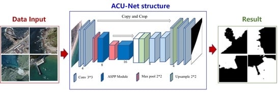
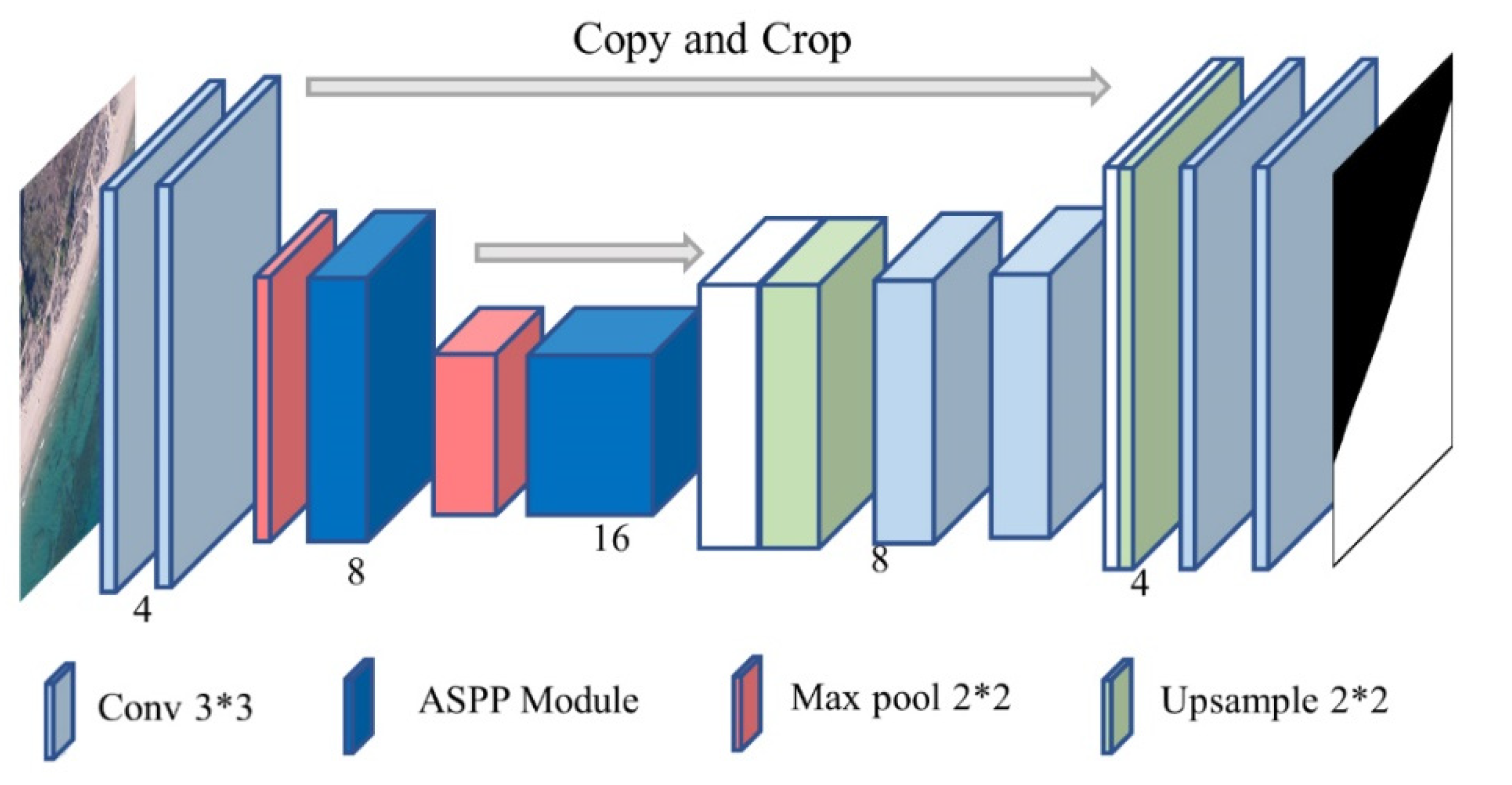
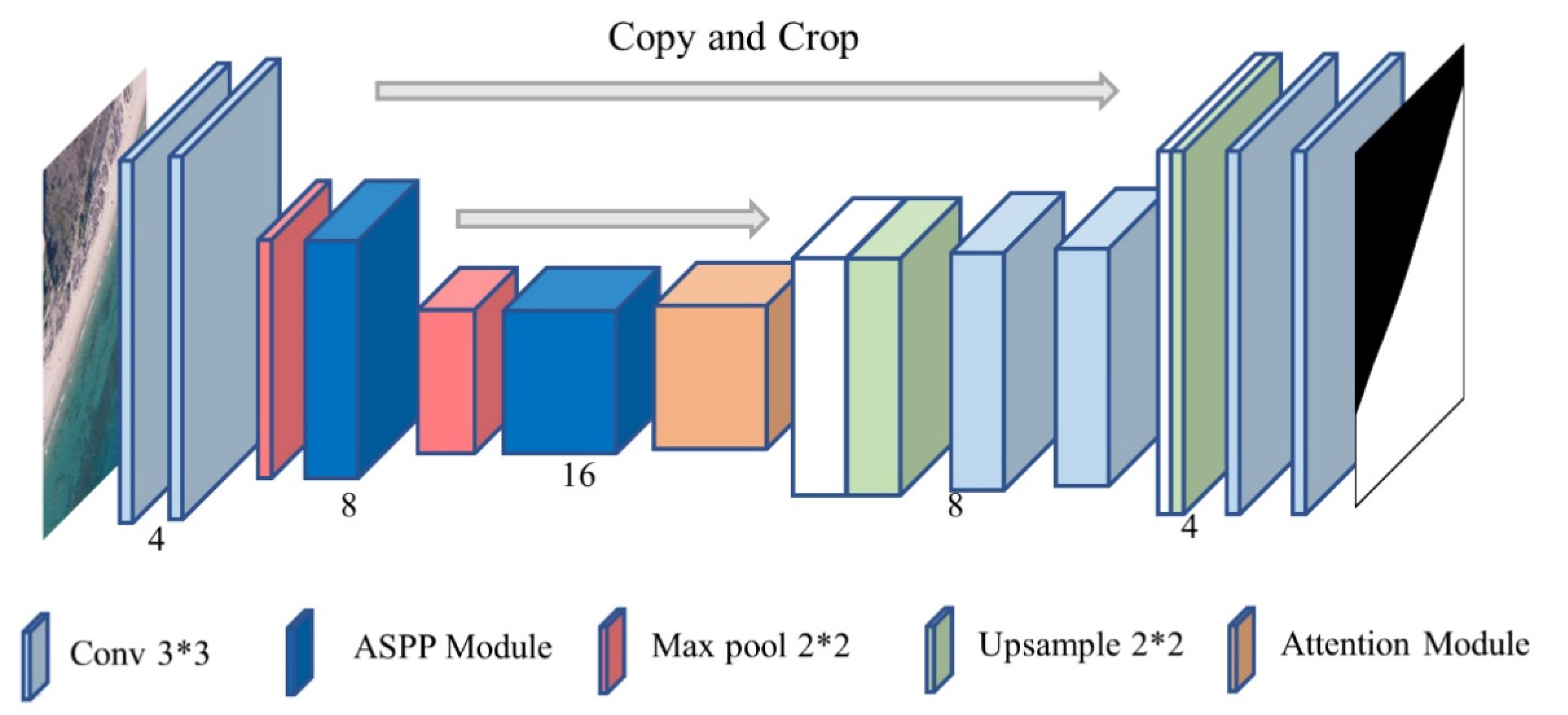
3. Methods
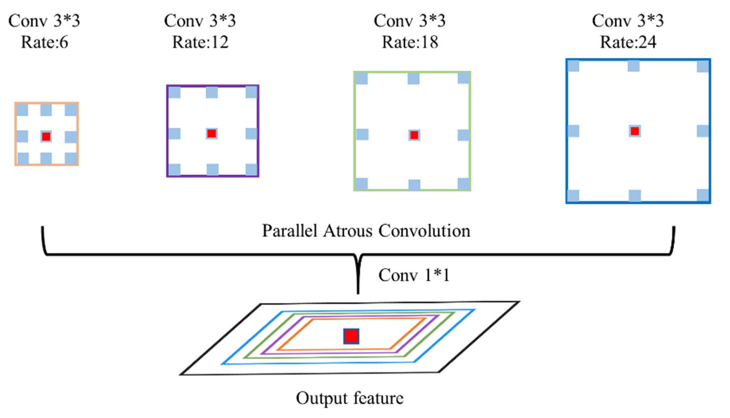
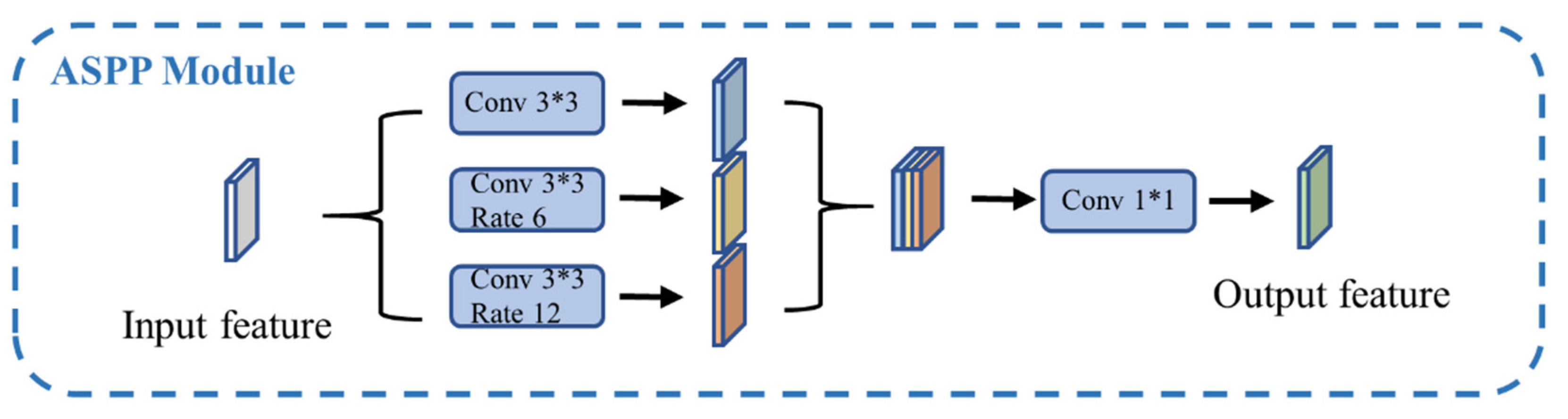
3.1. ASPP Module
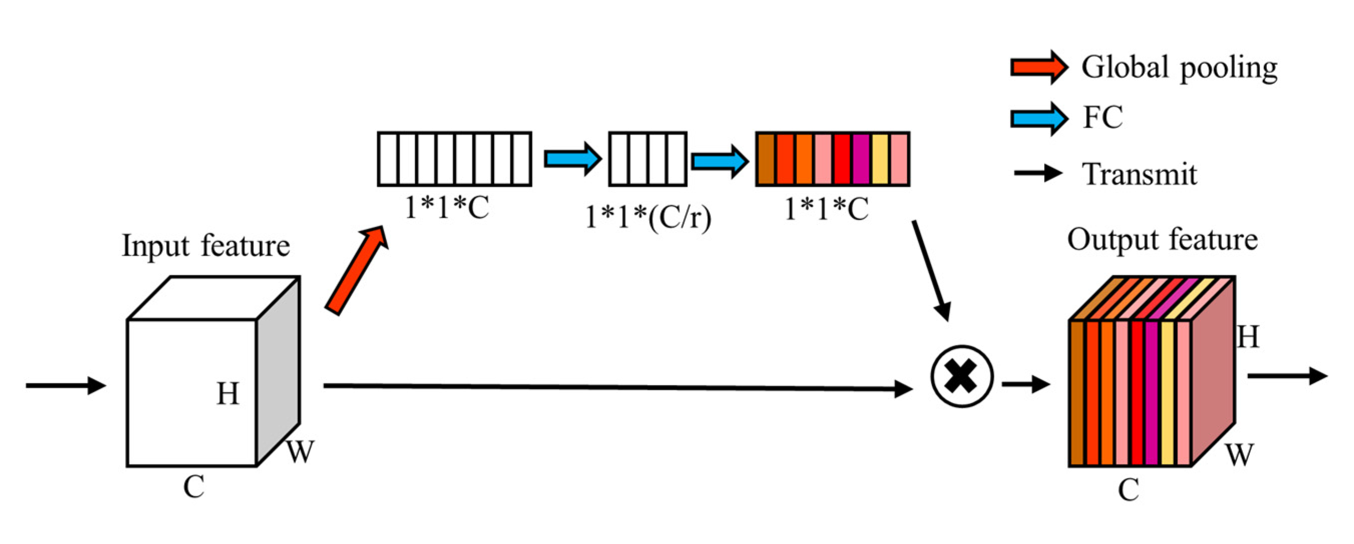
3.2. Attention Module
3.3. FReLU Activation Function
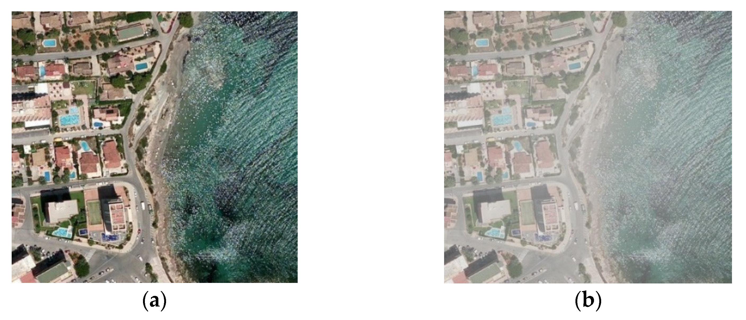
4. Results
4.1. Experimental Settings
4.2. Evaluation Index
4.3. Segmentation Results
4.4. Different Datasets
5. Discussion
Expansion Rate
6. Conclusions
Author Contributions
Funding
Data Availability Statement
Conflicts of Interest
References
- Li, M.; Zhu, D. Review on Image Semantic Segmentation Based on Fully Convolutional Network. Comput. Syst. Appl. 2021, 3, 41–52. [Google Scholar] [CrossRef]
- Liu, Q.; Zhang, X.; Wang, Y. A Sea-land Segmentation Method of SAR Image Based on Prior Information and U-Net. Radio Eng. 2021, 5, 1471–1476. [Google Scholar] [CrossRef]
- Nobuyuki, O. A Threshold Selection Method from Gray Level Histograms. IEEE Trans. Syst. Man Cybern. 1979, 9, 62–66. [Google Scholar] [CrossRef]
- Chen, X.; Sun, J.; Yi, K. Sea-Land Segmentation Algorithm of SAR Image Based on Otsu Method and Statistical Characteristic of Sea Area. J. Data Acquis. Processing 2014, 29, 603–608. [Google Scholar] [CrossRef]
- Li, J. Research on Sea-Land and Sea-Cloud Segmentation for High Resolution Ocean Remote Sensing Image. Master’s Thesis, Shenzhen University, Shenzhen, China, 2018. [Google Scholar]
- Pang, Y.; Liu, C. Modified Sea-land Segmentation Method based on the Super-pixel for SAR Images. Foreign Electron. Meas. Technol. 2019, 38, 12–18. [Google Scholar] [CrossRef]
- Kim, Y. Convolutional Neural Networks for Sentence Classification. In Proceedings of the EMNLP, Doha, Qatar, 25–29 October 2014. [Google Scholar]
- Kalchbrenner, N.; Grefenstette, E.; Blunsom, P. A Convolutional Neural Network for Modelling Sentences. arXiv 2014, arXiv:1404.2188. [Google Scholar]
- Evan, S.; Jonathan, L.; Trevor, D. Fully Convolutional Networks for Semantic Segmentation. IEEE Trans. Pattern Anal. Mach. Intell. 2017, 39, 640–651. [Google Scholar] [CrossRef]
- Ronneberger, O.; Fischer, P.; Brox, T. U-Net: Convolutional Networks for Biomedical Image Segmentation. In Proceedings of the 18th International Conference on Medical Image Computing and Computer-Assisted Intervention, Munich, Germany, 5–9 October 2015. [Google Scholar] [CrossRef]
- Vijay, B.; Alex, K.; Roberto, C. SegNet: A Deep Convolutional Encoder-Decoder Architecture for Image Segmentation. IEEE Trans. Pattern Anal. Mach. Intell. 2017, 39, 2481–2495. [Google Scholar] [CrossRef]
- Schuegraf, P.; Bittner, K. Automatic Building Footprint Extraction from Multi-Resolution Remote Sensing Images Using a Hybrid FCN. ISPRS Int. J. Geo Inf. 2017, 8, 191. [Google Scholar] [CrossRef]
- Li, M. Research on Semantic Segmentation Technology of Aerial Images Based on Deep Learning. Master’s Thesis, University of Chinese Academy of Sciences, Beijing, China, 2018. [Google Scholar] [CrossRef]
- Zhang, G. Research on Key Technologies of Remote Sensing Image Semantic Segmentation Based on Deep Learning. Ph.D. Thesis, University of Chinese Academy of Sciences, Beijing, China, 2020. [Google Scholar] [CrossRef]
- Peng, H. Research on Semantic Segmentation and Improvement of Aerial Remote Sensing Image Based on Fully Convolutional Neural Network. Master’s Thesis, Harbin Institute of Technology, Harbin, China, 2020. [Google Scholar]
- Wang, L. Research on Semantic Segmentation of Remote Sensing Images of the Ground Objects Based on Deeplab V3+ Network. Master’s Thesis, Harbin Institute of Technology, Harbin, China, 2020. [Google Scholar] [CrossRef]
- Wang, J.; Wu, F.; Teng, M.; Zhang, C. Remote Sensing Image Segmentation Method Using Improved PSPNet with ConvCRF. Geomat. World 2021, 28, 58–85. [Google Scholar] [CrossRef]
- Sun, K.; Xiao, B.; Liu, D.; Wang, J. Deep High-Resolution Representation Learning for Human Pose Estimation. In Proceedings of the 2019 IEEE/CVF Conference on Computer Vision and Pattern Recognition (CVPR), Long Beach, CA, USA, 15–20 June 2019; pp. 5686–5696. [Google Scholar]
- Wang, S. Research on Key Technologies of Satellite Image Semantic Refined Segmentation Based on Deep Learning. Master’s Thesis, Beijing University of Posts and Telecommunications, Beijing, China, 2020. [Google Scholar]
- Ma, N.; Zhang, X.; Sun, J. Funnel Activation for Visual Recognition. In Proceedings of the 16th European Conference on Computer Vision, Glasgow, UK, 23–28 August 2020. [Google Scholar] [CrossRef]
- Gallego, A.-J.; Pertusa, A.; Gil, P. Automatic Ship Classification from Optical Aerial Images with Convolutional Neural Networks. Remote Sens. 2018, 10, 511. [Google Scholar] [CrossRef]
- Cheng, G.; Han, J.; Lu, X. Remote Sensing Image Scene Classification: Benchmark and State of the Art. Proc. IEEE 2017, 105, 1865–1883. [Google Scholar] [CrossRef]
- Chen, L.; Zhu, Y.; Papandreou, G.; Schroff, F.; Adam, H. Encoder-Decoder with Atrous Separable Convolution for Semantic Image Segmentation. In Proceedings of the 15th European Conference on Computer Vision, Munich, Germany, 8–14 September 2018. [Google Scholar] [CrossRef]
- Chen, L.; Papandreou, G.; Kokkinos, I.; Murphy, K.; Yuille, A. DeepLab: Semantic Image Segmentation with Deep Convolutional Nets, Atrous Convolution, and Fully Connected CRFs. IEEE Trans. Pattern Anal. Mach. Intell. 2018, 40, 834–848. [Google Scholar] [CrossRef] [PubMed]
- Hu, J.; Shen, L.; Albanie, S.; Sun, G.; Wu, E. Squeeze-and-Excitation Networks. IEEE Trans. Pattern Anal. Mach. Intell. 2020, 42, 2011–2023. [Google Scholar] [CrossRef] [PubMed]
- Woo, S.; Park, J.; Lee, J.; Kweon, I. CBAM: Convolutional Block Attention Module. In Proceedings of the 15th European Conference on Computer Vision, Munich, Germany, 8–14 September 2018. [Google Scholar] [CrossRef] [Green Version]
- Park, J.; Woo, S.; Lee, J.; Kweon, I. BAM: Bottleneck Attention Module. arXiv 2018, arXiv:1807.06514. [Google Scholar]
- Wang, X.; Girshick, R.; Gupta, A.; He, K. Non-local Neural Networks. In Proceedings of the 2018 IEEE/CVF Conference on Computer Vision and Pattern Recognition, Salt Lake City, UT, USA, 18–23 June 2018. [Google Scholar] [CrossRef]
- Hou, Q.; Zhou, D.; Feng, J. Coordinate Attention for Efficient Mobile Network Design. In Proceedings of the 2021 IEEE/CVF Conference on Computer Vision and Pattern Recognition, Nashville, TN, USA, 20–25 June 2021. [Google Scholar] [CrossRef]
- Wang, Q.; Wu, B.; Zhu, P.; Li, P.; Zuo, W.; Hu, Q. ECA-Net: Efficient Channel Attention for Deep Convolutional Neural Networks. In Proceedings of the 2020 IEEE/CVF Conference on Computer Vision and Pattern Recognition, Seattle, WA, USA, 13–19 June 2020. [Google Scholar] [CrossRef]
- Fu, J.; Liu, J.; Tian, H.; Li, Y.; Bao, Y.; Fang, Z.; Lu, H. Dual Attention Network for Scene Segmentation. In Proceedings of the 2019 IEEE/CVF Conference on Computer Vision and Pattern Recognition, Long Beach, CA, USA, 15–20 June 2019. [Google Scholar] [CrossRef]
- Abadi, M.; Agarwal, A.; Barham, P.; Brevdo, E.; Chen, Z.; Citro, C.; Corrado, G.S.; Davis, A.; Dean, J.; Devin, M.; et al. TensorFlow: Large-Scale Machine Learning on Heterogeneous Distributed Systems. arXiv 2016, arXiv:1603.04467. [Google Scholar]
- Zhou, Z.; Siddiquee, M.; Tajbakhsh, N.; Liang, J. UNet plus plus: A Nested U-Net Architecture for Medical Image Segmentation. In Proceedings of the 4th International Workshop on Deep Learning in Medical Image Analysis/8th International Workshop on Multimodal Learning for Clinical Decision Support, Granada, Spain, 20 September 2018. [Google Scholar] [CrossRef] [Green Version]


| Name | Requirements |
|---|---|
| Operating Platform | Linux |
| Graphics Card | Nvidia 3090 |
| Graphics Memory | 8G |
| CUDA | 11.1 |
| cuDNN | 8.2.0 |
| HDD Capacity | 1T |
| Learning Framework | TensorFlow [32] |
| Framework Version | 2.7.0 |
| Language and Version | Python 3.7 |
| Model Structure | Size (MB) | Acc(%) | Loss(%) Dice + Ce | IoU |
|---|---|---|---|---|
| U-Net (4, 1024) | 355 | 96.026 | 10.417 | 0.936 |
| U-Net (4, 512) | 89 | 96.278 | 9.773 | 0.929 |
| U-Net (4, 256) | 22.4 | 97.059 | 8.293 | 0.940 |
| U-Net (3, 128) | 5.76 | 95.998 | 10.909 | 0.915 |
| U-Net (3, 64) | 1.6 | 95.726 | 11.698 | 0.909 |
| U-Net (3, 32) | 0.514 | 95.115 | 12.230 | 0.906 |
| U-Net (2, 16) | 0.208 | 94.633 | 12.710 | 0.880 |
| Model Structure | Size (MB) | Acc(%) | Loss(%) Dice + Ce | IoU |
|---|---|---|---|---|
| U-Net (3, 32) | 0.514 | 95.115 | 12.230 | 0.906 |
| U-Net++ [33] (3, 32) | 0.645 | 95.757 | 11.301 | 0.912 |
| ACU-Net (3, 32) Rates (1, 4, 8) | 0.613 | 96.365 | 10.644 | 0.927 |
| ACU-Net (3, 32) Rates (1, 6, 12) | 0.613 | 96.474 | 9.412 | 0.927 |
| Model Structure | Size (MB) | Acc(%) | Loss(%) Dice + Ce | IoU |
|---|---|---|---|---|
| U-Net (3, 32) | 0.514 | 95.115 | 12.230 | 0.906 |
| U-Net (3, 32) (FReLU) | 0.710 | 96.374 | 9.164 | 0.926 |
| U-Net++ (3, 32) | 0.645 | 95.757 | 11.301 | 0.912 |
| ACU-Net (3, 32) Rates (1, 4, 8) | 0.613 | 96.365 | 10.644 | 0.927 |
| ACU-Net (3, 32) Rates (1, 6, 12) | 0.613 | 96.474 | 9.412 | 0.927 |
| ACU-Net (3, 32) (FReLU) Rates (1, 4, 8) | 0.901 | 96.637 | 9.112 | 0.932 |
| ACU-Net (3, 32) (FReLU) Rates (1, 6, 12) | 0.901 | 96.716 | 8.141 | 0.929 |
| ACU-Net (2, 16) (FReLU) Rates (1, 4, 8) | 0.444 | 96.762 | 8.873 | 0.933 |
| ACU-Net (2, 16) (FReLU) Rates (1, 6, 12) | 0.444 | 96.859 | 7.773 | 0.935 |
| Model Structure | Size (MB) | Acc(%) | Loss(%) Dice + Ce | IoU |
|---|---|---|---|---|
| DeeplabV3+ | 480 | 96.579 | 8.928 | 0.932 |
| U-Net (4, 512) | 89 | 96.278 | 9.773 | 0.929 |
| U-Net++ (4, 512) | 103 | 97.402 | 7.925 | 0.944 |
| U-Net (3, 32) | 0.514 | 95.115 | 12.230 | 0.906 |
| U-Net (3, 32) (FReLU) | 0.710 | 96.374 | 9.164 | 0.926 |
| U-Net + SE (3, 32) | 0.536 | 96.023 | 8.495 | 0.917 |
| U-Net++ (3, 32) | 0.645 | 95.757 | 11.301 | 0.912 |
| ACU-Net (2, 16) | 0.444 | 96.859 | 7.773 | 0.935 |
| ACU-Net (2, 16) + SE | 0.477 | 96.986 | 7.602 | 0.938 |
| Serial Number | Model Structure | Size (MB) | Acc(%) | Loss(%) Dice + Ce | IoU (100) | IoU (Average) |
|---|---|---|---|---|---|---|
| a | DeeplabV3+ | 480 | 96.579 | 8.928 | 0.908 | 0.932 |
| b | U-Net | 89 | 96.278 | 9.773 | 0.860 | 0.929 |
| c | U-Net++ | 103 | 97.402 | 7.925 | 0.877 | 0.945 |
| d | U-Net(downsize) | 0.514 | 95.115 | 12.230 | 0.834 | 0.906 |
| e | U-Net(downsize, FReLU) | 0.710 | 96.374 | 9.164 | 0.865 | 0.923 |
| f | U-Net++(downsize) | 0.645 | 95.757 | 11.301 | 0.842 | 0.911 |
| g | ACU-Net | 0.444 | 96.859 | 7.773 | 0.861 | 0.935 |
| f | ACU-Net+SE | 0.477 | 96.986 | 7.602 | 0.870 | 0.938 |
| Model Structure | Size (MB) | Acc(%) | Loss(%) Dice + Ce | IoU (100) | IoU (Average) |
|---|---|---|---|---|---|
| ACU-Net (3, 32) (FReLU) Rates (1, 4, 8) | 0.901 | 96.637 | 9.112 | 0.877 | 0.932 |
| ACU-Net (3, 32) (FReLU) Rates (1, 6, 12) | 0.901 | 96.716 | 8.141 | 0.876 | 0.929 |
| ACU-Net (2, 16) (FReLU) Rates (1, 4, 8) | 0.444 | 96.762 | 8.873 | 0.874 | 0.933 |
| ACU-Net (2, 16) (FReLU) Rates (1, 6, 12) | 0.444 | 96.859 | 7.773 | 0.861 | 0.935 |
Publisher’s Note: MDPI stays neutral with regard to jurisdictional claims in published maps and institutional affiliations. |
© 2022 by the authors. Licensee MDPI, Basel, Switzerland. This article is an open access article distributed under the terms and conditions of the Creative Commons Attribution (CC BY) license (https://creativecommons.org/licenses/by/4.0/).
Share and Cite
Li, J.; Huang, Z.; Wang, Y.; Luo, Q. Sea and Land Segmentation of Optical Remote Sensing Images Based on U-Net Optimization. Remote Sens. 2022, 14, 4163. https://doi.org/10.3390/rs14174163
Li J, Huang Z, Wang Y, Luo Q. Sea and Land Segmentation of Optical Remote Sensing Images Based on U-Net Optimization. Remote Sensing. 2022; 14(17):4163. https://doi.org/10.3390/rs14174163
Chicago/Turabian StyleLi, Jianfeng, Zhenghong Huang, Yongling Wang, and Qinghua Luo. 2022. "Sea and Land Segmentation of Optical Remote Sensing Images Based on U-Net Optimization" Remote Sensing 14, no. 17: 4163. https://doi.org/10.3390/rs14174163