
Coupled Tensor Block Term Decomposition with Superpixel-Based Graph Laplacian Regularization for Hyperspectral Super-Resolution

Abstract
:
1. Introduction
1.1. Relates Works
1.2. Motivations and Contributions
- (1)
- The MSI is segmented by regional clustering according to spectral–spatial distance measurements;
- (2)
- Two-directional tensor graphs are designed via the features of the segmented MSI superpixel blocks, whose local geometric structure is consistent with HSI;
- (3)
- The similarity weights of the superpixel blocks are calculated and graph Laplacian matrices are constructed, which is used to convey the spatial manifold structures from MSI to the factor matrices of HSI;
- (4)
- The proposed superpixel graph Laplacian BTD model is solved by the block coordinate descent algorithm, and the experimental results are displayed.
2. Background
2.1. Block Term Decomposition
2.2. Problem Formulation
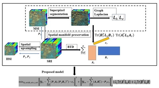
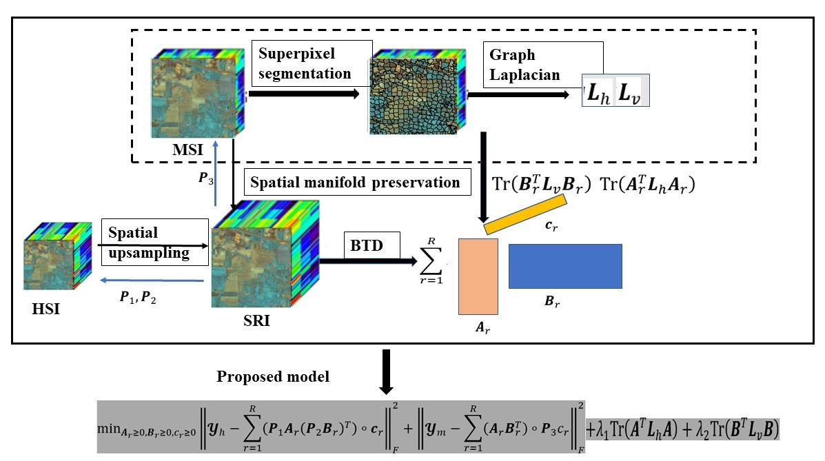
3. Proposed Methods
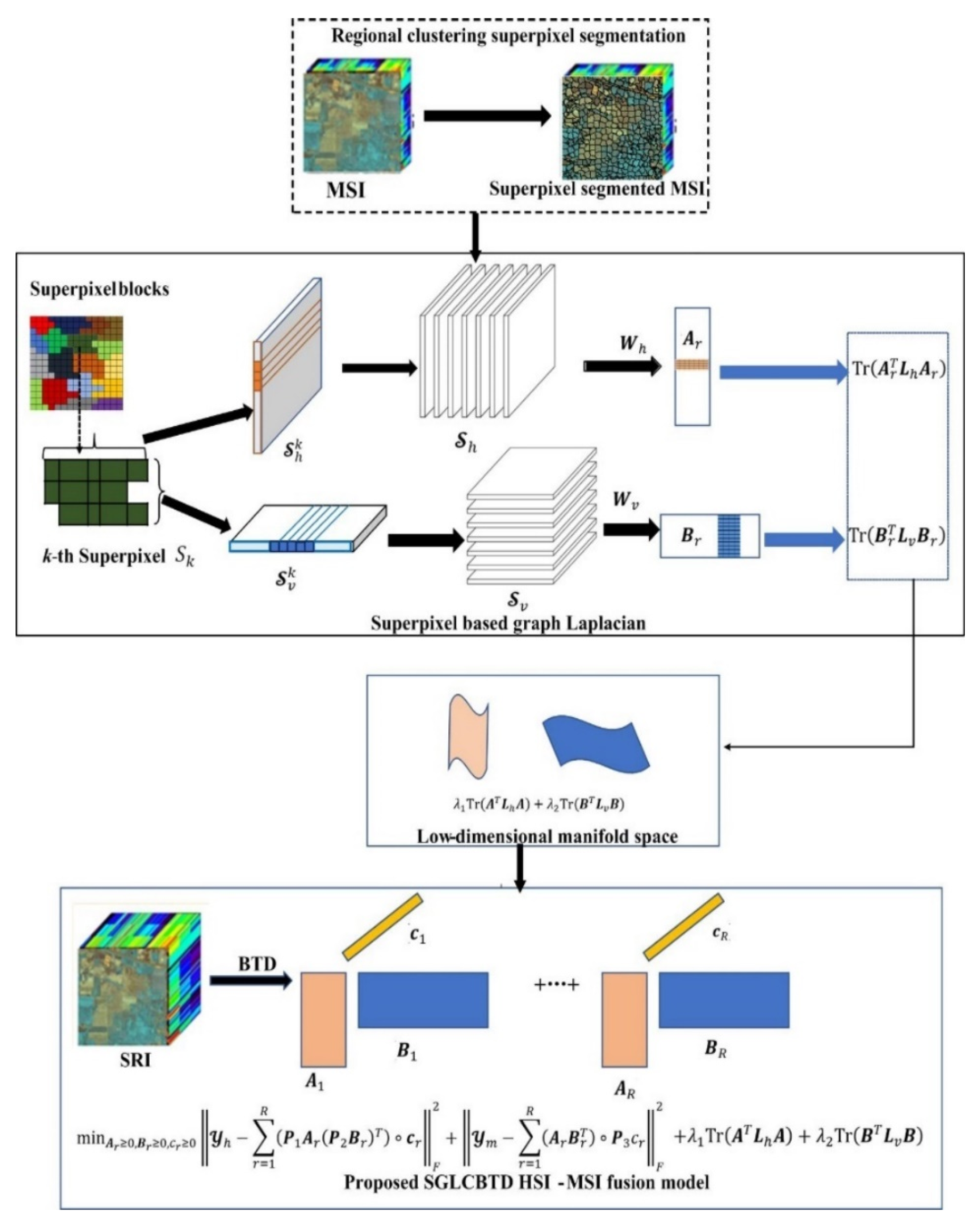
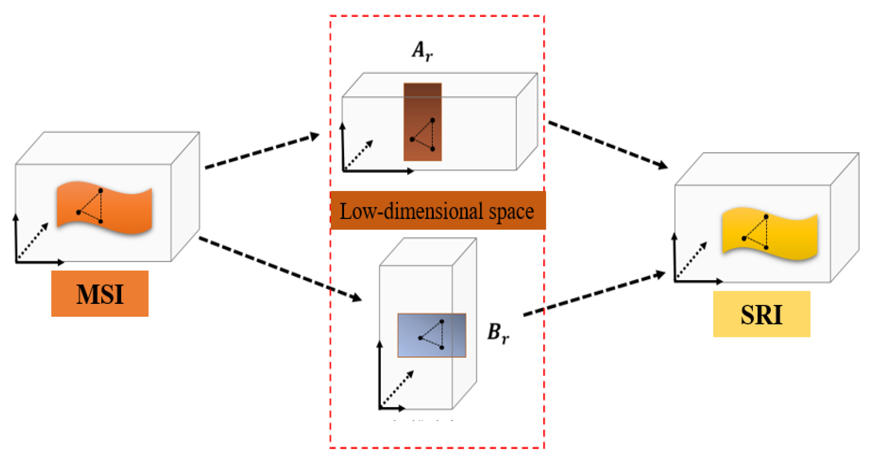
3.1. Superpixel-Based Graph Laplician Construction
3.1.1. Regional Clustering-Based Superpixel Segmentation
3.1.2. Two-Directional Feature Tensors Extraction
3.1.3. Two Graph Generation
3.1.4. Two Graph Laplacian Construction
3.2. Proposed SGLCBTD Model and Algorithm
4. Experimental Results
4.1. Experiment Setup
4.1.1. Quality Assessment Indices
- (1)
- Normalized mean square error (NMSE) is defined aswhere is the ideal HSI and is the resulted SRI.
- (2)
- Reconstruction signal-to-noise ratio (R-SNR) is inversely proportional to NMSE with the formulation as follows:
- (3)
- Spectral angle mapper (SAM) evaluates the spectral distortion and is defined aswhere is the spectral vector, is inner product of two vectors.
- (4)
- Relative global dimensional synthesis error (ERGAS) reflects the global quality of the fused results and is defined aswhere is spatial upsampling factor, is the mean of .
- (5)
- Correlation coefficient (CC) is computed as followswhere is the Pearson correlation coefficient.
- (6)
- Peak signal-to-noise rate (PSNR) for each band of HSI is defined as
- (7)
- Structural similarity index measurement (SSIM) for each band of HSI is defined as follows:where and are the mean and variance of the k-th band image and , respectively, is the covariance between and , and are constant.
4.1.2. Methods for Comparison
4.2. Performance Comparison of Different Methods
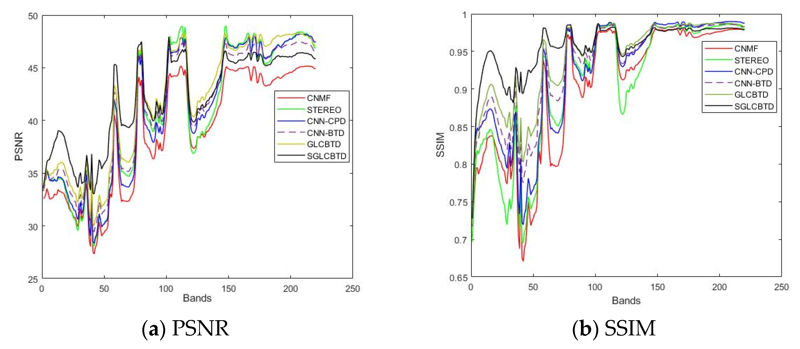
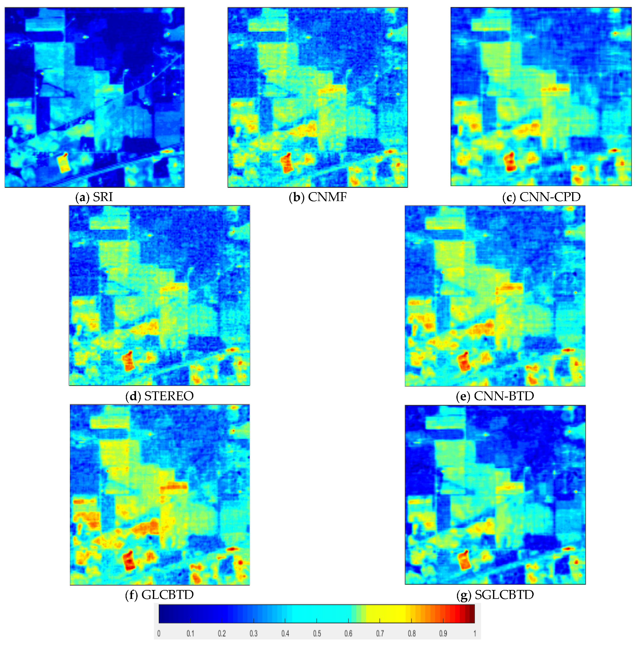
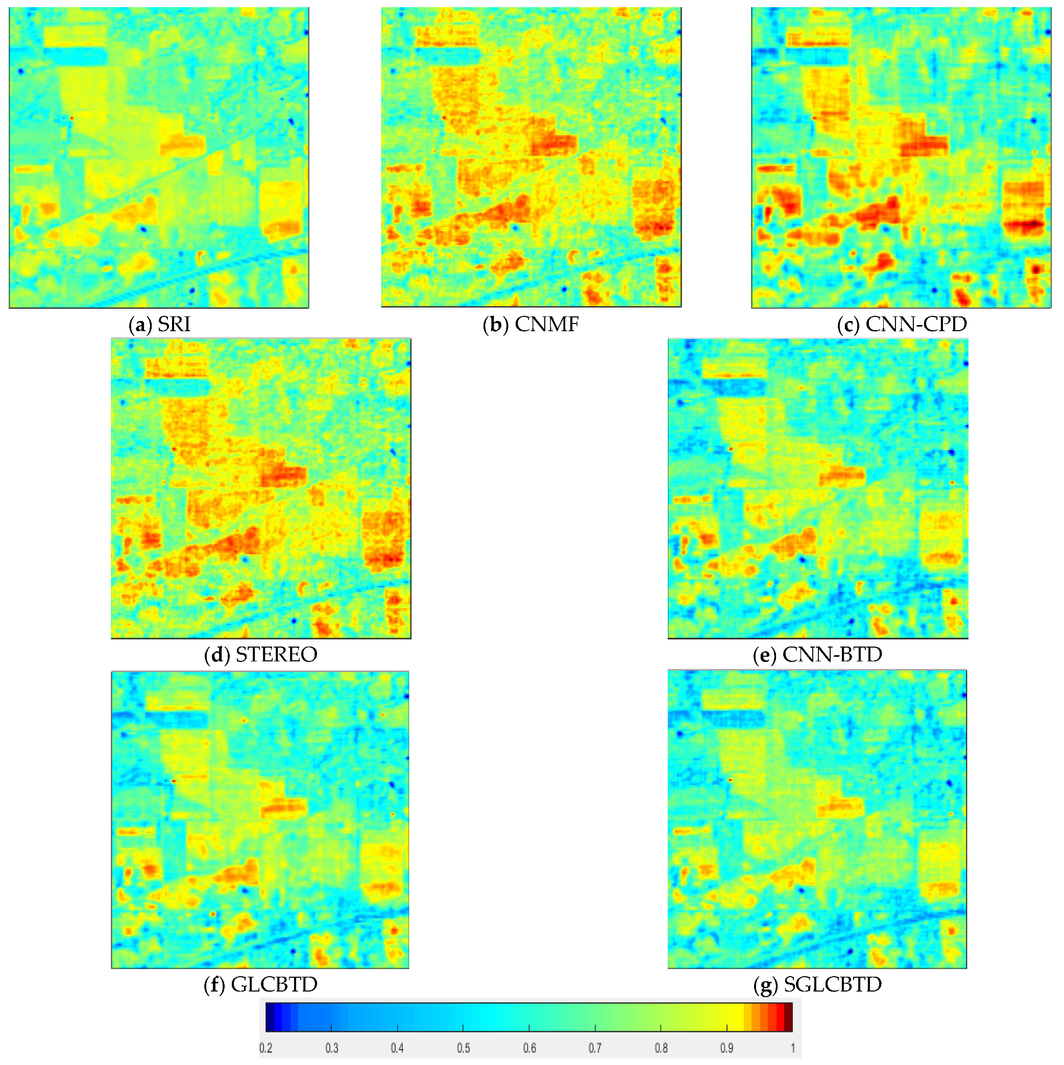
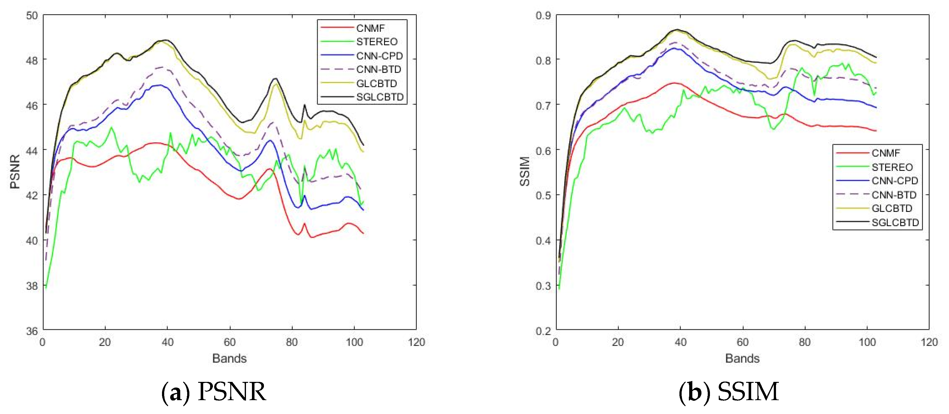
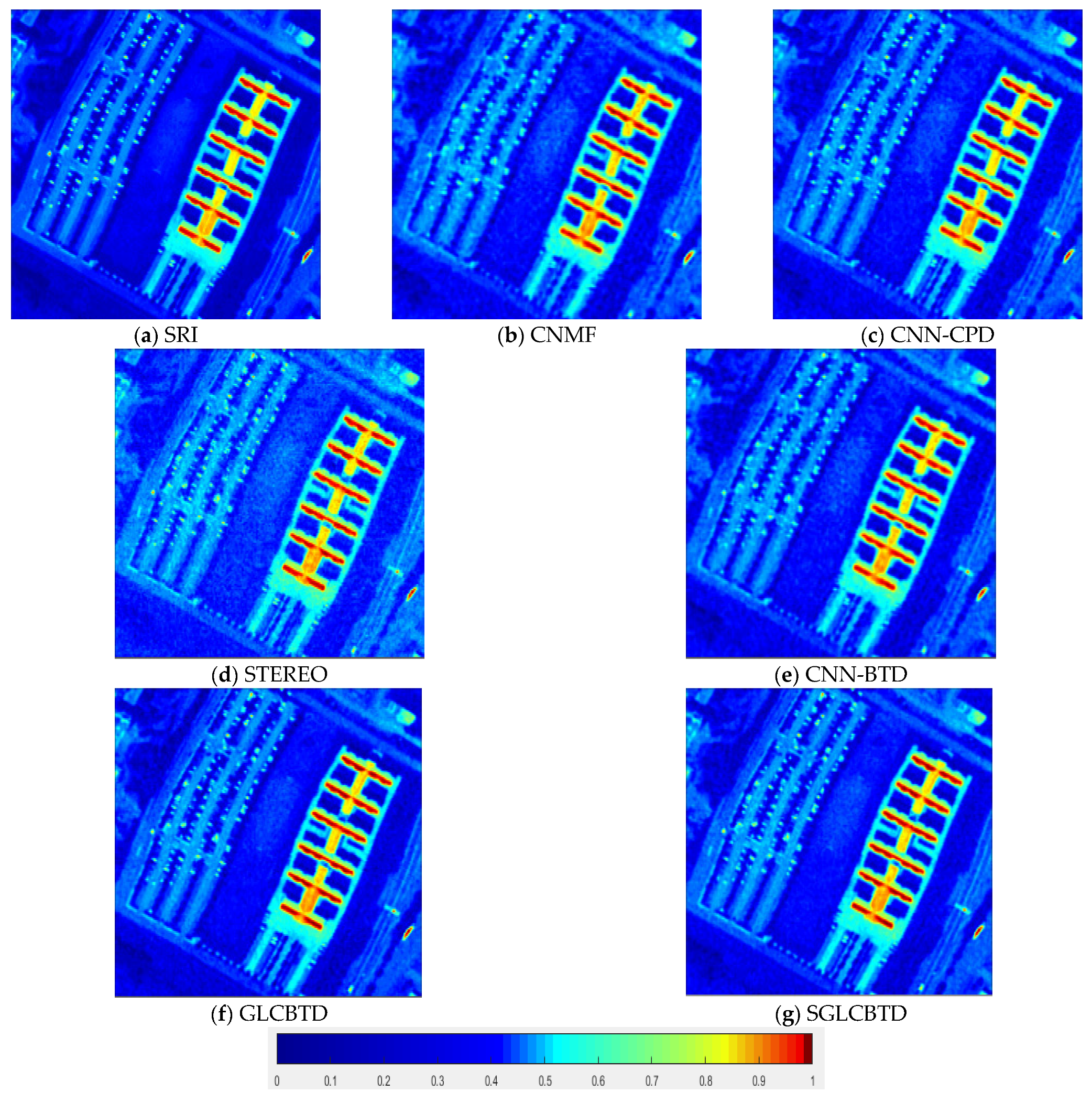
4.2.1. Indian Pines Dataset
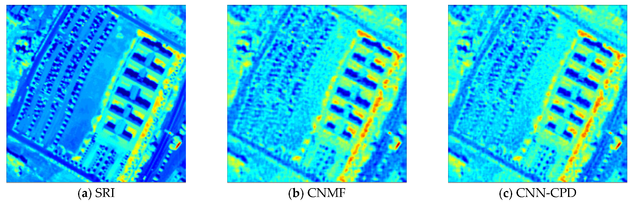
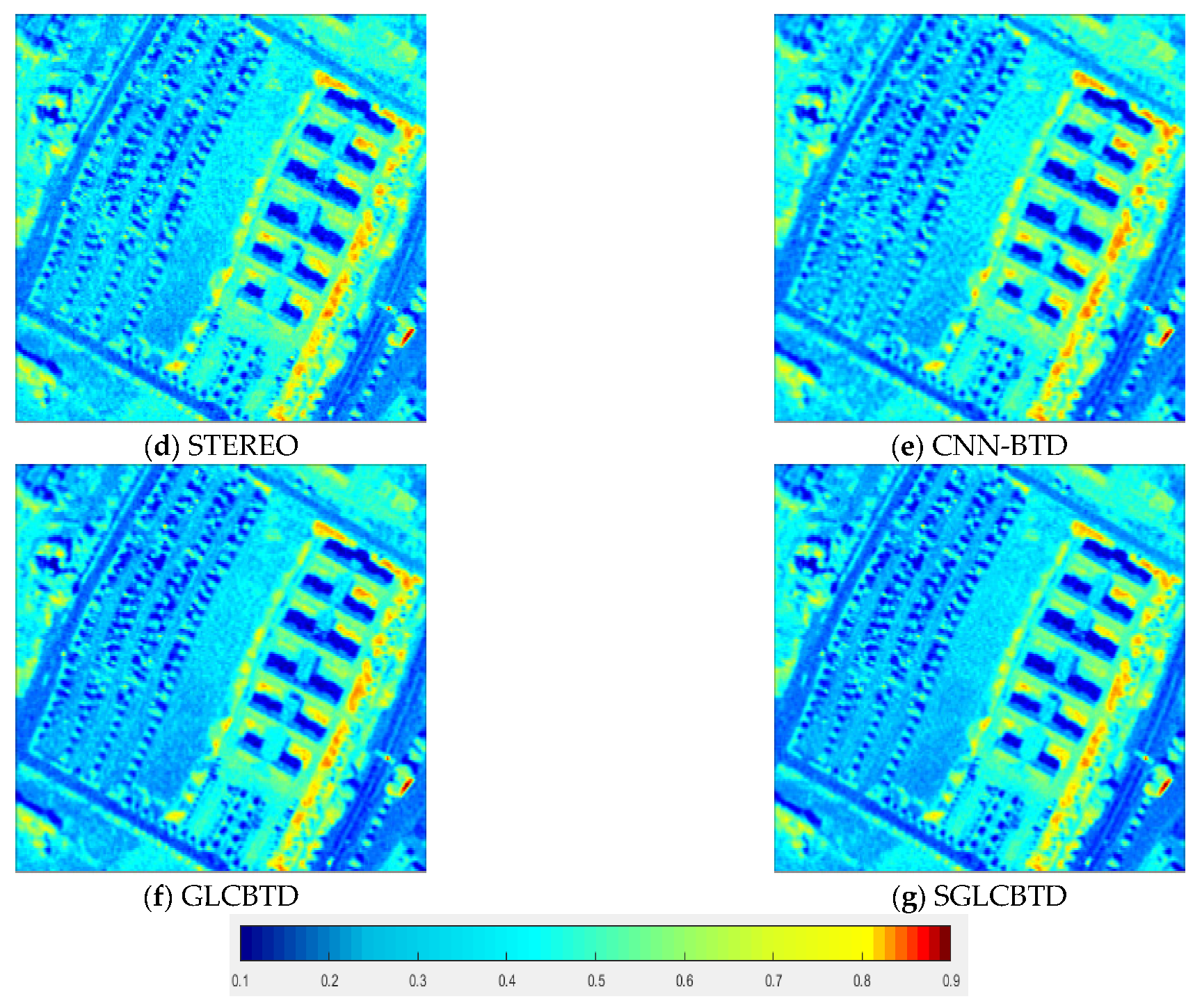
4.2.2. Pavia University Dataset
4.3. Discussions
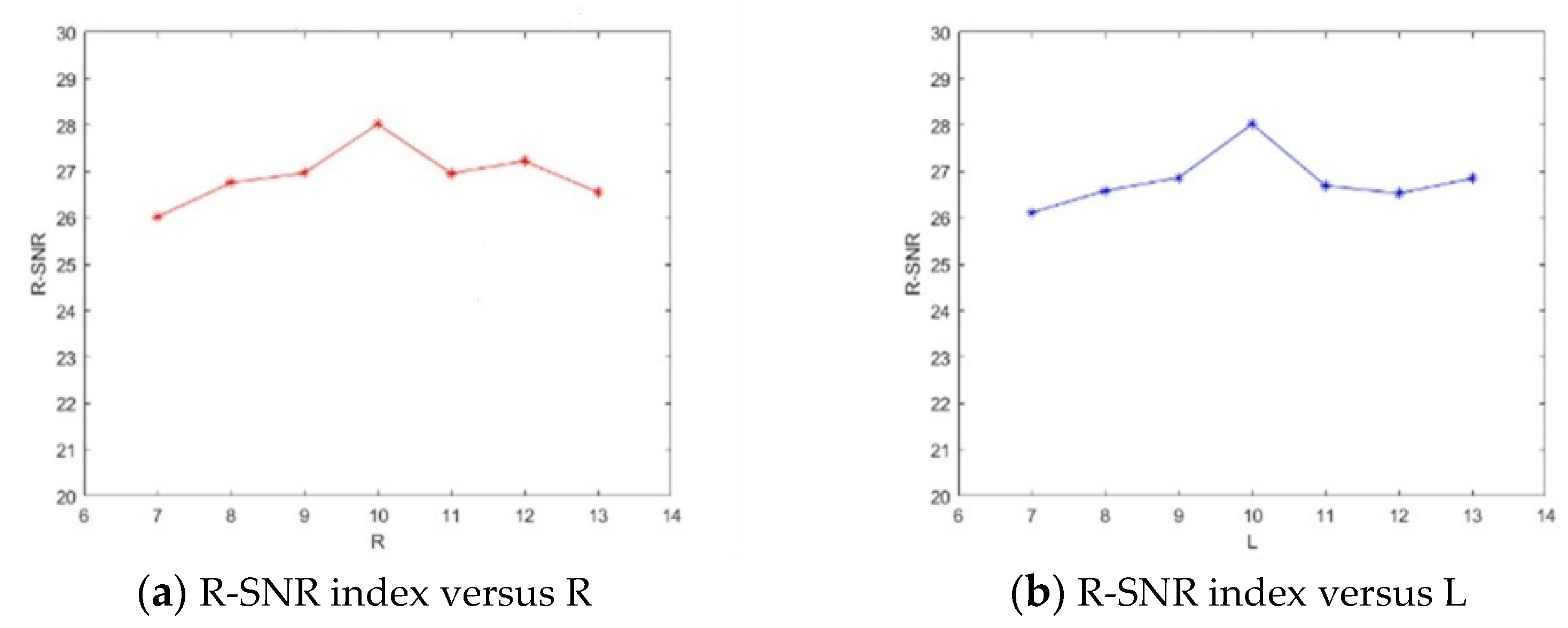
4.3.1. Parameter Analysis
- (1)
- Analysis of R and L
- (2)
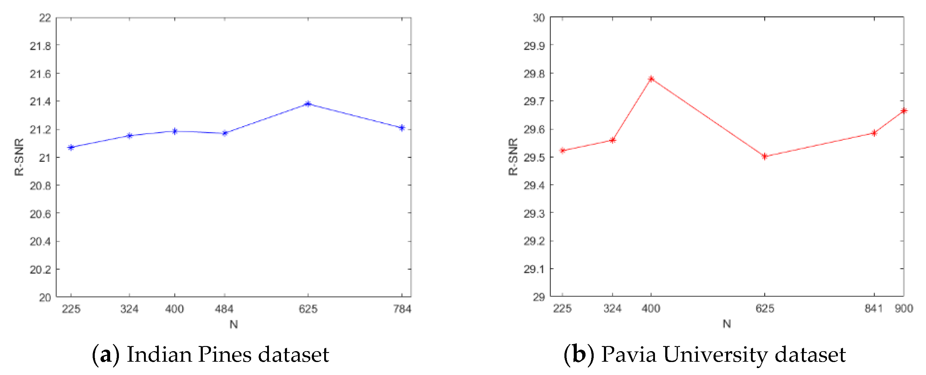
- Analysis of N
4.3.2. Time Complexity Analysis
5. Conclusions
Author Contributions
Funding
Data Availability Statement
Conflicts of Interest
References
- Chen, S.; Chang, C.I.; Li, X. Component Decomposition Analysis for Hyperspectral Anomaly Detection. IEEE Geosci. Remote Sens. 2022, 60, 5516222. [Google Scholar] [CrossRef]
- He, C.; Sun, L.; Huang, W.; Zhang, J.; Zheng, Y.; Jeon, B. TSLRLN: Tensor subspace low-rank learning with non-local prior for hyperspectral image mixed denoising. Signal Process. 2021, 184, 108060. [Google Scholar] [CrossRef]
- Yokoya, N.; Yairi, T.; Iwasaki, A. Coupled Non-negative Matrix Factorization Unmixing for Hyperspectral and Multispectral Data Fusion. IEEE Trans. Geosci. Remote Sens. 2012, 50, 528–537. [Google Scholar] [CrossRef]
- Wei, Q.; Bioucas-Dias, J.M.; Dobigeon, N.; Tourneret, J. Hyperspectral and Multispectral Image Fusion based on a Sparse Representation. IEEE Trans. Geosci. Remote Sens. 2015, 53, 3658–3668. [Google Scholar] [CrossRef]
- Dian, R.; Li, T.; Sun, B.; Guo, A.J. Recent Advances and New Guidelines on Hyperspectral and Multispectral Image Fusion. Inf. Fusion 2021, 69, 40–51. [Google Scholar] [CrossRef]
- Vivone, G.; Alparone, L.; Chanussot, J.; Dalla Mura, M.; Garzelli, A.; Licciardi, G.A.; Restaino, R.; Wald, L. A Critical Comparison Among Pansharpening Algorithms. IEEE Trans. Geosci. Remote Sens. 2015, 53, 2565–2586. [Google Scholar] [CrossRef]
- Yokoya, N.; Grohnfeldt, C.; Chanussot, J. Hyperspectral and Multispectral Data Fusion: A Comparative Review of the Recent Literature. IEEE Geosci. Remote Sens. Mag. 2017, 5, 29–56. [Google Scholar] [CrossRef]
- Zhang, Y.; He, M. Multi-Spectral and Hyperspectral Image Fusion Using 3-D Wavelet Transform. J. Electron. 2007, 24, 218–224. [Google Scholar] [CrossRef]
- Selva, M.; Aiazzi, B.; Butera, F.; Chiarantini, L.; Baronti, S. Hyper-sharpening: A First Approach on SIM-GA Data. IEEE J. Sel. Top. Appl. Earth Obs. Remote Sens. 2015, 8, 3008–3024. [Google Scholar] [CrossRef]
- Zou, C.; Xia, Y. Hyperspectral Image Super-Resolution Based on Double Regularization Unmixing. IEEE Geosci. Remote Sens. Lett. 2017, 14, 1022–1026. [Google Scholar] [CrossRef]
- Huang, B.; Song, H.; Cui, H.; Peng, J.; Xu, Z. Spatial and Spectral Image Fusion Using Sparse Matrix Factorization. IEEE Trans. Geosci. Remote Sens. 2014, 52, 1693–1704. [Google Scholar] [CrossRef]
- Dong, W.; Fu, F.; Shi, G.; Cao, X.; Wu, J.; Li, G.; Li, X. Hyperspectral Image Super-Resolution via Non-Negative Structured Sparse Representation. IEEE Trans. Image Process. 2016, 25, 2337–2352. [Google Scholar] [CrossRef] [PubMed]
- Dian, R.; Fang, L.; Li, S. Hyperspectral Image Super-Resolution via Non-Local Sparse Tensor Factorization. In Proceedings of the 2017 IEEE Conference on Computer Vision and Pattern Recognition (CVPR), Hawaii, HI, USA, 21–26 July 2017; pp. 3862–3871. [Google Scholar]
- Li, S.; Dian, R.; Fang, L.; Bioucas-Dias, J.M. Fusing Hyperspectral and Multispectral Images via Coupled Sparse Tensor Factorization. IEEE Trans. Image Process. 2018, 27, 4118–4130. [Google Scholar] [CrossRef] [PubMed]
- Chang, Y.; Yan, L.; Zhao, X.; Fang, H.; Zhang, Z.; Zhong, S. Weighted Low-Rank Tensor Recovery for Hyperspectral Image Restoration. IEEE Trans. Cybern. 2020, 50, 4558–4572. [Google Scholar] [CrossRef] [PubMed]
- Prvost, C.; Usevich, K.; Comon, P.; Brie, D. Hyperspectral Super-Resolution with Coupled Tucker Approximation: Recoverability and SVD-Based Algorithms. IEEE Trans. Signal Process. 2020, 68, 931–946. [Google Scholar] [CrossRef]
- Zhang, K.; Wang, M.; Yang, S.; Jiao, L. Spatial–Spectral-Graph-Regularized Low-Rank Tensor Decomposition for Multispectral and Hyperspectral Image Fusion. IEEE J. Sel. Top. Appl. Earth Obs. Remote Sens. 2018, 11, 1030–1040. [Google Scholar] [CrossRef]
- Palsson, F.; Sveinsson, J.R.; Ulfarsson, M.O. Multispectral and Hyperspectral Image Fusion using a 3D-Convolutional Neural Network. IEEE Geosci. Remote Sens. Lett. 2017, 14, 639–643. [Google Scholar] [CrossRef]
- Mei, S.; Yuan, X.; Ji, J.; Wan, S.; Hou, J.; Du, Q. Hyperspectral Image Super-Resolution via Convolutional Neural Network. In Proceedings of the 2017 IEEE International Conference on Image Processing (ICIP), Beijing, China, 17–20 September 2017; pp. 4297–4301. [Google Scholar]
- Xu, Y.; Wu, Z.; Chanussot, J.; Zhi, H. Nonlocal Patch Tensor Sparse Representation for Hyperspectral Image Super-Resolution. IEEE Trans. Image Process. 2019, 28, 3034–3047. [Google Scholar] [CrossRef]
- Dian, R.W.; Li, S.T.; Fang, L.Y.; Lu, T.; Bioucas-Dias, J.M. Nonlocal Sparse Tensor Factorization for Semiblind Hyperspectral and Multispectral Images Fusion. IEEE Trans. Cybern. 2020, 50, 4469–4480. [Google Scholar] [CrossRef]
- Long, J.; Peng, Y.; Li, J.; Zhang, L.; Xu, Y. Hyperspectral Image Super-Resolution via Subspace-based Fast Low Tensor Multi-Rank Regularization. Infrared Phys. Technol. 2021, 116, 103631. [Google Scholar] [CrossRef]
- Liu, N.; Li, L.; Li, W.; Tao, R.; Flower, J.; Chanussot, J. Hyperspectral Restoration and Fusion with Multispectral Imagery via Low-Rank Tensor-Approximation. IEEE Trans. Geosci. Remote Sens. 2021, 59, 7817–7830. [Google Scholar] [CrossRef]
- Liu, H.; Sun, P.; Du, Q.; Wu, Z.; Wei, Z. Hyperspectral Image Restoration Based on Low-Rank Recovery with a Local Neighborhood Weighted Spectral-Spatial Total Variation Model. IEEE Trans. Geosci. Remote Sens. 2019, 57, 1409–1422. [Google Scholar] [CrossRef]
- Fang, L.; Zhuo, H.; Li, S. Super-Resolution of Hyperspectral Image via Superpixel-based Sparse Representation. Neurocomputing 2017, 273, 171–177. [Google Scholar] [CrossRef]
- Li, X.; Zhang, Y.; Ge, Z.; Cao, G.; Shi, H.; Fu, P. Adaptive Nonnegative Sparse Representation for Hyperspectral Image Super-Resolution. IEEE J. Sel. Top. Appl. Earth Obs. Remote Sens. 2021, 14, 4267–4283. [Google Scholar] [CrossRef]
- Peng, J.T.; Sun, W.W.; Li, H.C.; Li, W.; Meng, X.; Ge, C.; Du, Q. Low-Rank and Sparse Representation for Hyperspectral Image Processing: A review. IEEE Geosci. Remote Sens. Mag. 2022, 10, 10–43. [Google Scholar] [CrossRef]
- Bu, Y.; Zhao, Y. Hyperspectral and Multispectral Image Fusion via Graph Laplacian-Guided Coupled Tensor Decomposition. IEEE Trans. Geosci. Remote Sens. 2021, 59, 648–662. [Google Scholar] [CrossRef]
- Li, C.; Jiang, Y.; Chen, X. Hyperspectral Unmixing via Noise-Free Model. IEEE Trans. Geosci. Remote Sens. 2021, 59, 3277–3291. [Google Scholar] [CrossRef]
- Fang, L.Y.; He, N.J.; Lin, H. CP Tensor-Based Compression of Hyperspectral Images. J. Opt. Soc. Am. A Opt. Image Sci. Vis. 2017, 34, 252–258. [Google Scholar] [CrossRef]
- Liu, H.Y.; Li, H.Y.; Wu, Z.B.; Wei, Z.H. Hyperspectral Image Recovery using Non-Convex Low-Rank Tensor Approximation. Remote Sens. 2020, 12, 2264. [Google Scholar] [CrossRef]
- Sun, L.; Cheng, Q.; Chen, Z. Hyperspectral Image Super-Resolution Method based on Spectral Smoothing Prior and Tensor Tubal Row-Sparse Representation. Remote Sens. 2022, 14, 2142. [Google Scholar] [CrossRef]
- Xu, Y.; Wu, Z.; Chanussot, J.; Wei, Z.H. Hyperspectral Images Super-Resolution via Learning High-Order Coupled Tensor Ring Representation. IEEE Trans Neural Netw. Learn. Syst. 2020, 31, 4747–4760. [Google Scholar] [CrossRef] [PubMed]
- Chen, Y.; Zeng, J.; He, W.; Zhao, X.; Huang, T. Hyperspectral and Multispectral Image Fusion Using Factor Smoothed Tenson Ring Decomposition. IEEE Trans. Geosci. Remote Sens. 2022, 60, 1–17. [Google Scholar]
- Lathauwer, L.D. Decompositions of a Higher-Order Tensor in Block Terms—Part II: Definitions and Uniqueness. SIAM J. Matrix Anal. Appl. 2008, 30, 1033–1066. [Google Scholar] [CrossRef]
- Lathauwer, L.D.; Nion, D. Decompositions of a Higher-Order Tensor in Block Terms—Part III: Alternating Least Squares Algorithms. SIAM J. Matrix Anal. Appl. 2008, 30, 1067–1083. [Google Scholar] [CrossRef]
- Kanatsoulis, C.I.; Fu, X.; Sidiropoulos, N.D.; Ma, W. Hyperspectral Super-Resolution: A Coupled Tensor Factorization Approach. IEEE Trans. Signal Process. 2018, 66, 6503–6517. [Google Scholar] [CrossRef]
- Xu, Y.; Wu, Z.B.; Chanussot, J.; Comon, P.; Wei, Z.H. Nonlocal Coupled Tensor CP Decomposition for Hyperspectral and Multispectral Image Fusion. IEEE Trans. Geosci. Remote Sens. 2020, 58, 348–362. [Google Scholar] [CrossRef]
- Borsoi, R.A.; Pr’evost, C.; Usevich, K.; Brie, D.; Bermudez, J.M.; Richard, C. Coupled Tensor Decomposition for Hyperspectral and Multispectral Image Fusion with Inter-Image Variability. IEEE J. Sel. Top. Signal Process. 2021, 15, 702–717. [Google Scholar] [CrossRef]
- Zheng, P.; Su, H.J.; Du, Q. Sparse and Low-Rank Constrained Tensor Factorization for Hyperspectral Image Unmixing. IEEE J. Sel. Top. Appl. Earth Obs. Remote Sens. 2021, 14, 1754–1767. [Google Scholar] [CrossRef]
- Xiong, F.; Chen, J.Z.; Zhou, J.; Qian, Y. Superpixel-Based Nonnegative Tensor Factorization for Hyperspectral Unmixing. In Proceedings of the 2018 IEEE International Geoscience and Remote Sensing Symposium (IGARSS), Valencia, Spain, 22–27 July 2018; pp. 6392–6395. [Google Scholar]
- Qian, Y.; Xiong, F.; Zeng, S.; Zhou, J.; Tang, Y. Matrix-Vector Nonnegative Tensor Factorization for Blind Unmixing of Hyperspectral Imagery. IEEE Trans. Geosci. Remote Sens. 2017, 55, 1776–1792. [Google Scholar] [CrossRef]
- Zhang, G.; Fu, X.; Huang, K.; Wang, J. Hyperspectral Super-Resolution: A Coupled Nonnegative Block-Term Tensor Decomposition Approach. In Proceedings of the 2019 IEEE International Workshop on Computational Advances in Multi-Sensor Adaptive Processing (CAMSAP), Le Gosier, France, 15–18 December 2019; pp. 470–474. [Google Scholar]
- Prevost, C.; Borsoi, R.A.; Usevich, K.; Brie, D.; Bermudez, J.C.M.; Richard, C. Hyperspectral Super-Resolution Accounting for Spectral Variability: LL1-Based Recovery and Blind Unmixing of the Unknown Super-Resolution. SIAM J. Imag. Sci. 2022, 15, 110–138. [Google Scholar] [CrossRef]
- Ding, M.; Fu, X.; Huang, T.; Wang, J.; Zhao, X. Hyperspectral Super-Resolution via Interpretable Block-Term Tensor Modeling. IEEE J. Sel. Top. Signal Process. 2021, 15, 641–656. [Google Scholar] [CrossRef]
- Jiang, W.; Liu, H.; Zhang, J. Hyperspectral and Mutispectral Image Fusion via Coupled Block Term Decomposition with Graph Laplacian Regularization. In Proceedings of the 2021 SPIE International Conference on Signal Image Processing and Communication (ICSIPC 2021), Chengdu, China, 16–18 April 2021; p. 11848. [Google Scholar]
- Xu, X.; Li, J.; Wu, C.S.; Plazad, A. Regional Clustering-Based Spatial Preprocessing for Hyperspectral Unmixing. Remote Sens. Environ. 2018, 204, 333–346. [Google Scholar] [CrossRef]
- Xu, Y.Y. Alternating Proximal Gradient Method for Sparse Nonnegative Tucker Decomposition. Math. Prog. Comp. 2015, 7, 39–70. [Google Scholar] [CrossRef]
- Gardiner, J.D.; Laub, A.J.; Amato, J.J.; Moler, C.B. Solution of the Sylvester Matrix Equation AXBT + CXDT = E. ACM Trans. Math. Softw. 1992, 18, 223–231. [Google Scholar] [CrossRef]
- Wald, L.; Ranchin, T.; Mangolini, M. Fusion of Satellite Images of Different Spatial Resolutions: Assessing the Quality of Resulting Images. Photogramm. Eng. Remote Sens. 1997, 63, 691–699. [Google Scholar]


| Algorithm | R-SNR | NMSE | SAM | ERGAS | CC |
|---|---|---|---|---|---|
| CNMF | 25.24 | 0.0546 | 0.0398 | 1.3320 | 0.7589 |
| STEREO | 26.25 | 0.0487 | 0.0413 | 1.1254 | 0.7970 |
| CNN-CPD | 26.41 | 0.0478 | 0.0365 | 1.0891 | 0.7980 |
| CNN-BTD | 27.32 | 0.0430 | 0.0346 | 1.0394 | 0.8070 |
| GLCBTD | 28.02 | 0.0397 | 0.0319 | 0.9507 | 0.8193 |
| SGLCBTD | 29.78 | 0.0324 | 0.0277 | 0.9610 | 0.8128 |
| Algorithm | R-SNR | NMSE | SAM | ERGAS | CC |
|---|---|---|---|---|---|
| CNMF | 17.36 | 0.1355 | 0.1105 | 1.0453 | 0.9526 |
| STEREO | 18.21 | 0.1228 | 0.1465 | 1.0154 | 0.9624 |
| CNN-CPD | 18.75 | 0.1154 | 0.1052 | 0.8867 | 0.9652 |
| CNN-BTD | 19.41 | 0.1070 | 0.1042 | 0.8447 | 0.9702 |
| GLCBTD | 21.08 | 0.0883 | 0.0873 | 0.7100 | 0.9792 |
| SGLCBTD | 21.38 | 0.0853 | 0.0855 | 0.6919 | 0.9807 |
| Method | Indian Pines Dataset | Pavia University Dataset |
|---|---|---|
| CNMF | 9.02 | 11.34 |
| STEREO | 2.97 | 4.76 |
| CNN-CPD | 5.05 | 5.60 |
| CNN-BTD | 65 | 89 |
| GLCBTD | 534 | 771 |
| SGLCBTD | 1023 | 1245 |
Publisher’s Note: MDPI stays neutral with regard to jurisdictional claims in published maps and institutional affiliations. |
© 2022 by the authors. Licensee MDPI, Basel, Switzerland. This article is an open access article distributed under the terms and conditions of the Creative Commons Attribution (CC BY) license (https://creativecommons.org/licenses/by/4.0/).
Share and Cite
Liu, H.; Jiang, W.; Zha, Y.; Wei, Z. Coupled Tensor Block Term Decomposition with Superpixel-Based Graph Laplacian Regularization for Hyperspectral Super-Resolution. Remote Sens. 2022, 14, 4520. https://doi.org/10.3390/rs14184520
Liu H, Jiang W, Zha Y, Wei Z. Coupled Tensor Block Term Decomposition with Superpixel-Based Graph Laplacian Regularization for Hyperspectral Super-Resolution. Remote Sensing. 2022; 14(18):4520. https://doi.org/10.3390/rs14184520
Chicago/Turabian StyleLiu, Hongyi, Wen Jiang, Yuchen Zha, and Zhihui Wei. 2022. "Coupled Tensor Block Term Decomposition with Superpixel-Based Graph Laplacian Regularization for Hyperspectral Super-Resolution" Remote Sensing 14, no. 18: 4520. https://doi.org/10.3390/rs14184520