
Influence of Radar Parameters and Sea State on Wind Wave-Induced Velocity in C-Band ATI SAR Ocean Surface Currents

 ,
,
Abstract
:1. Introduction
2. Materials and Methods
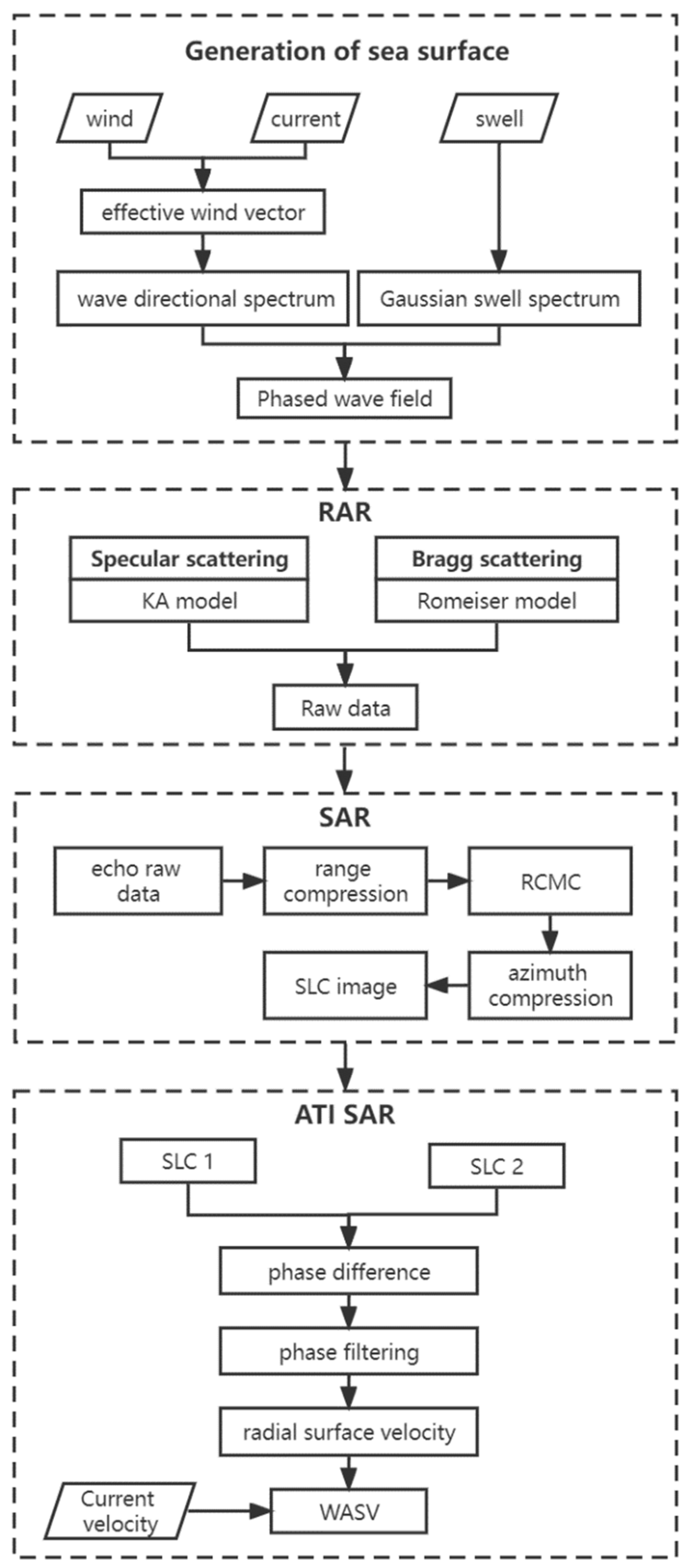
2.1. Ocean Surface Modeling
2.2. Scattering Model
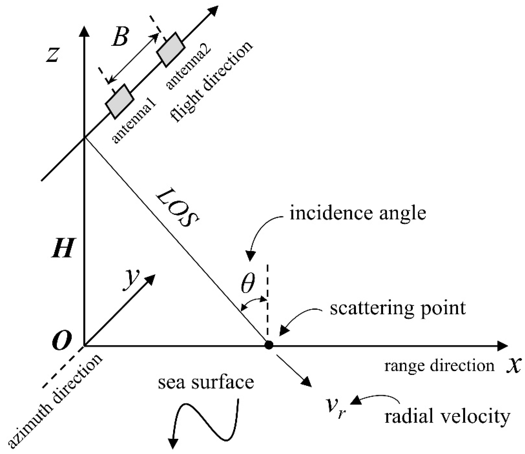
2.3. Retrieval of WASV from ATI SAR
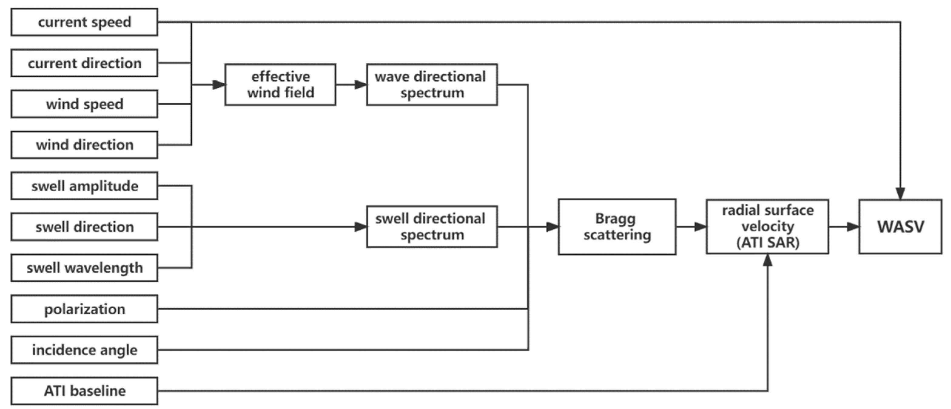
2.4. Simulation Parameters
3. Results
3.1. Influence of ATI SAR Parameters on WASV
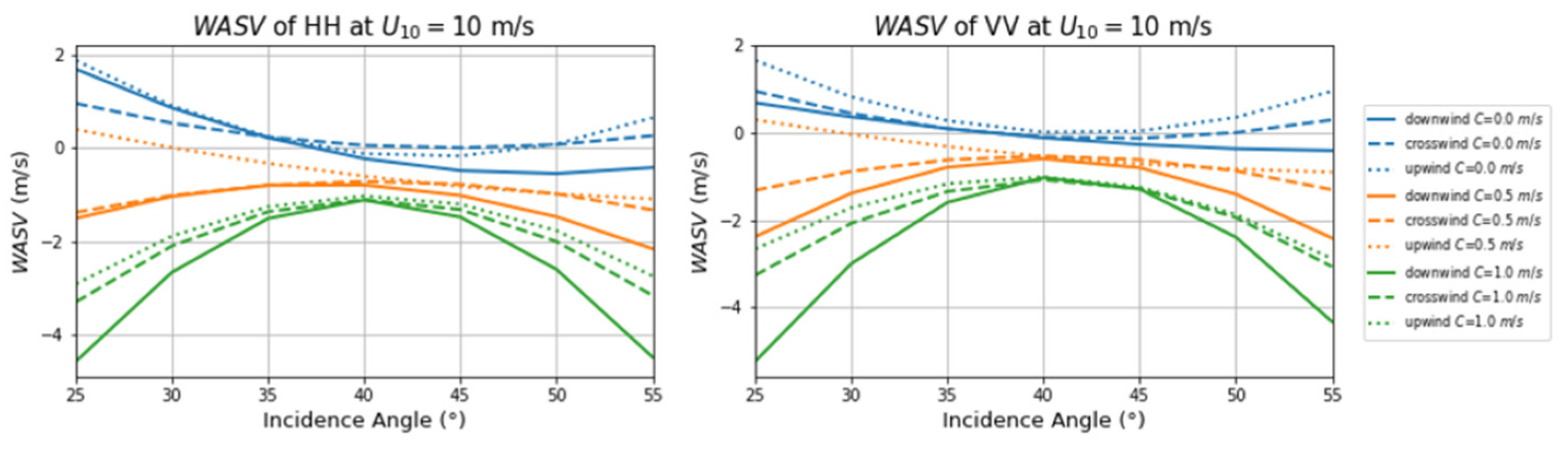
3.1.1. Incidence Angle
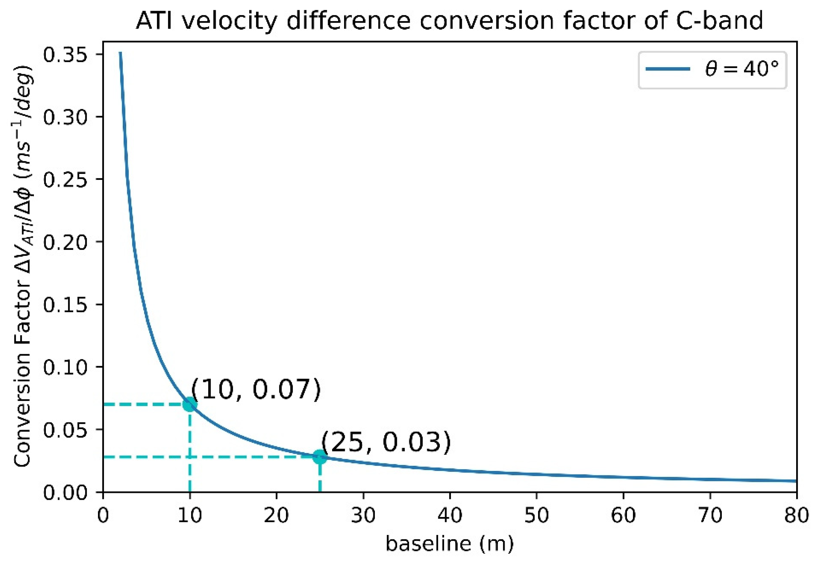
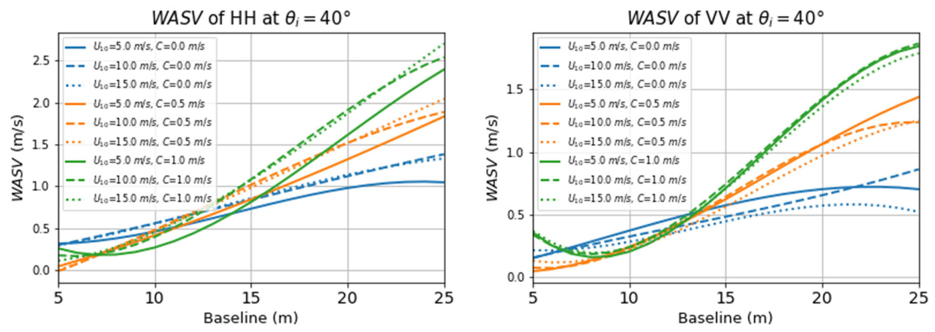
3.1.2. ATI SAR Baseline
3.2. Influence of Sea State on WASV
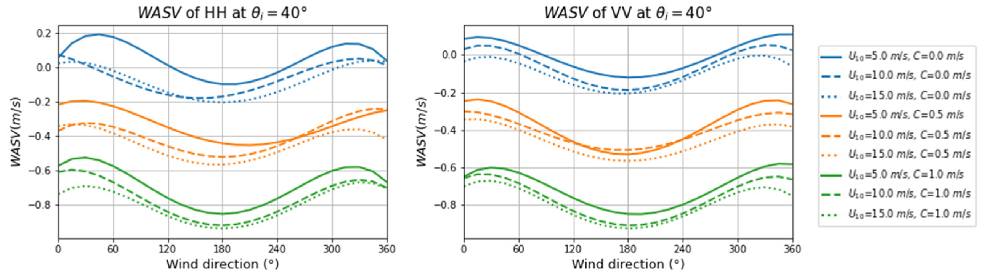
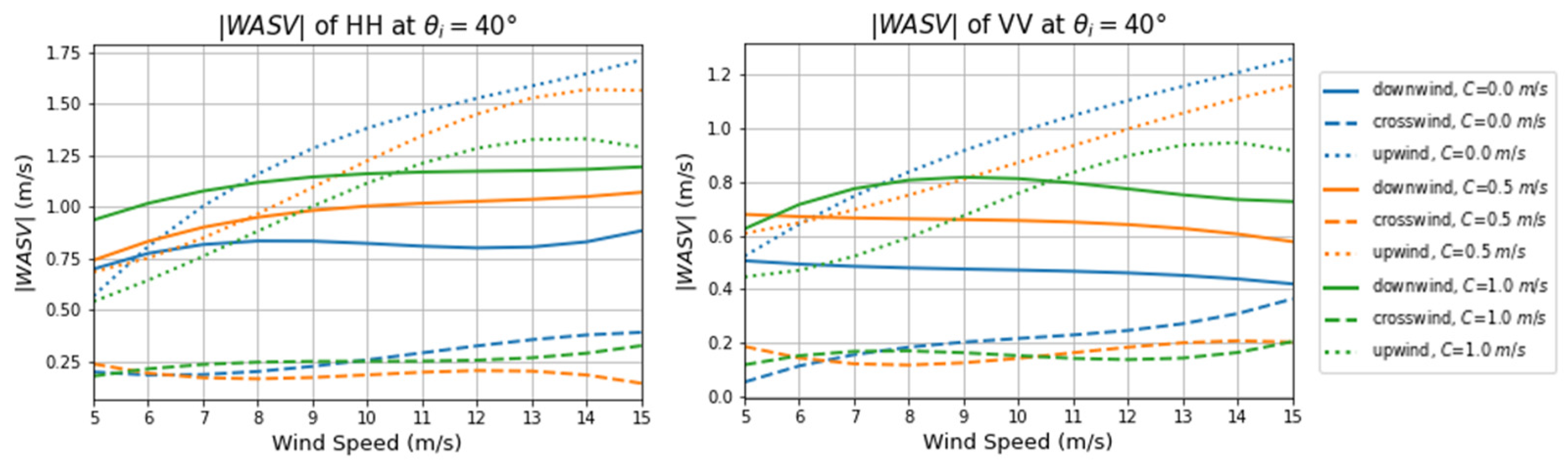
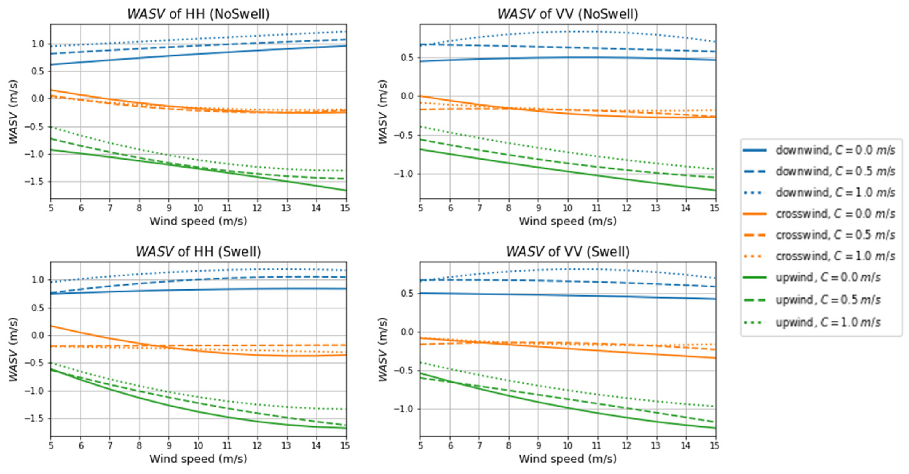
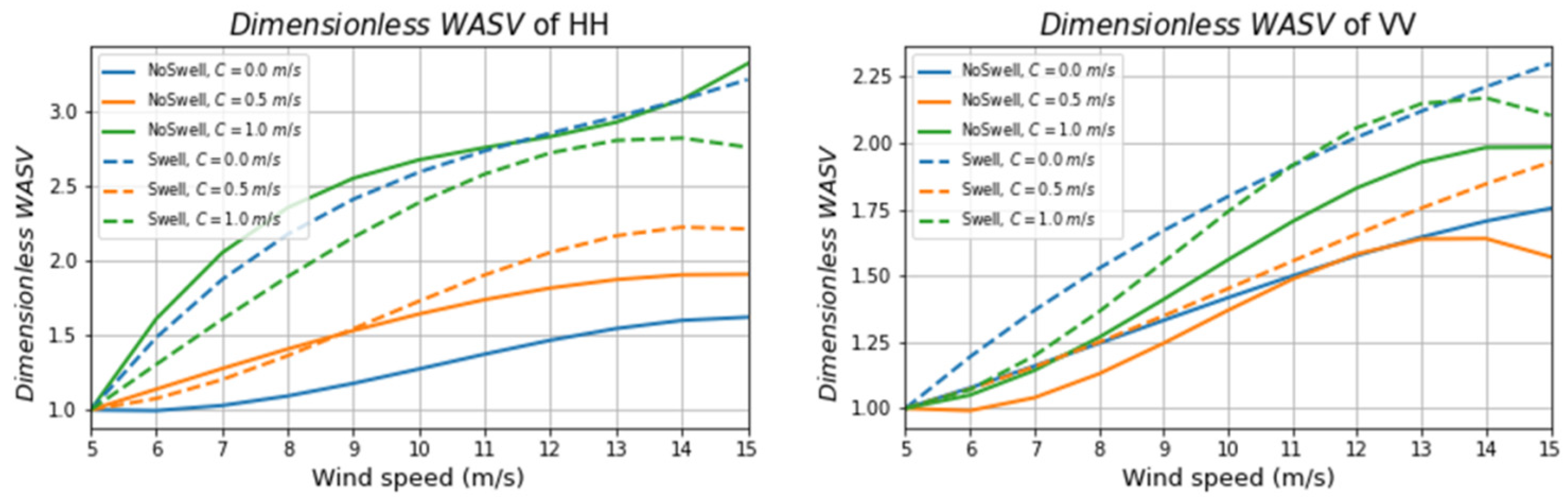
3.2.1. Wind Effect
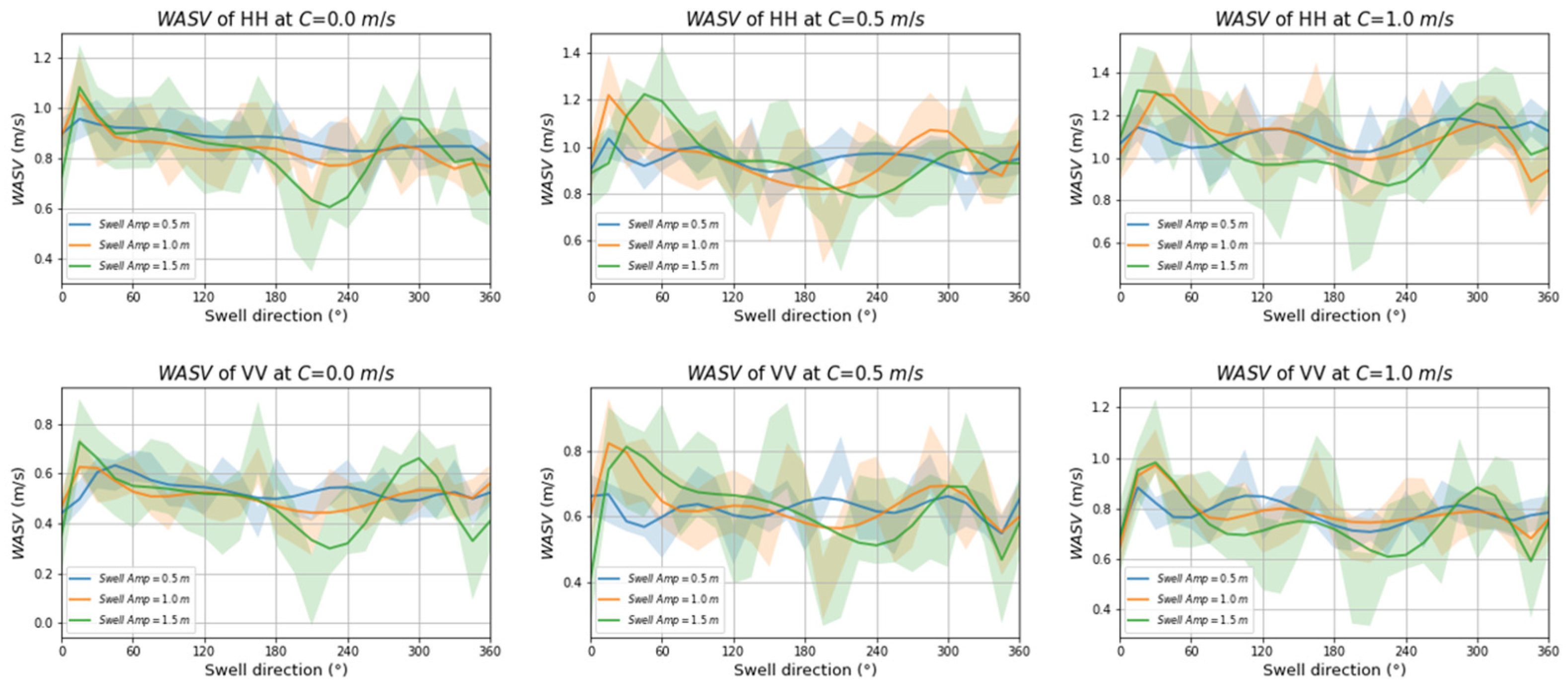
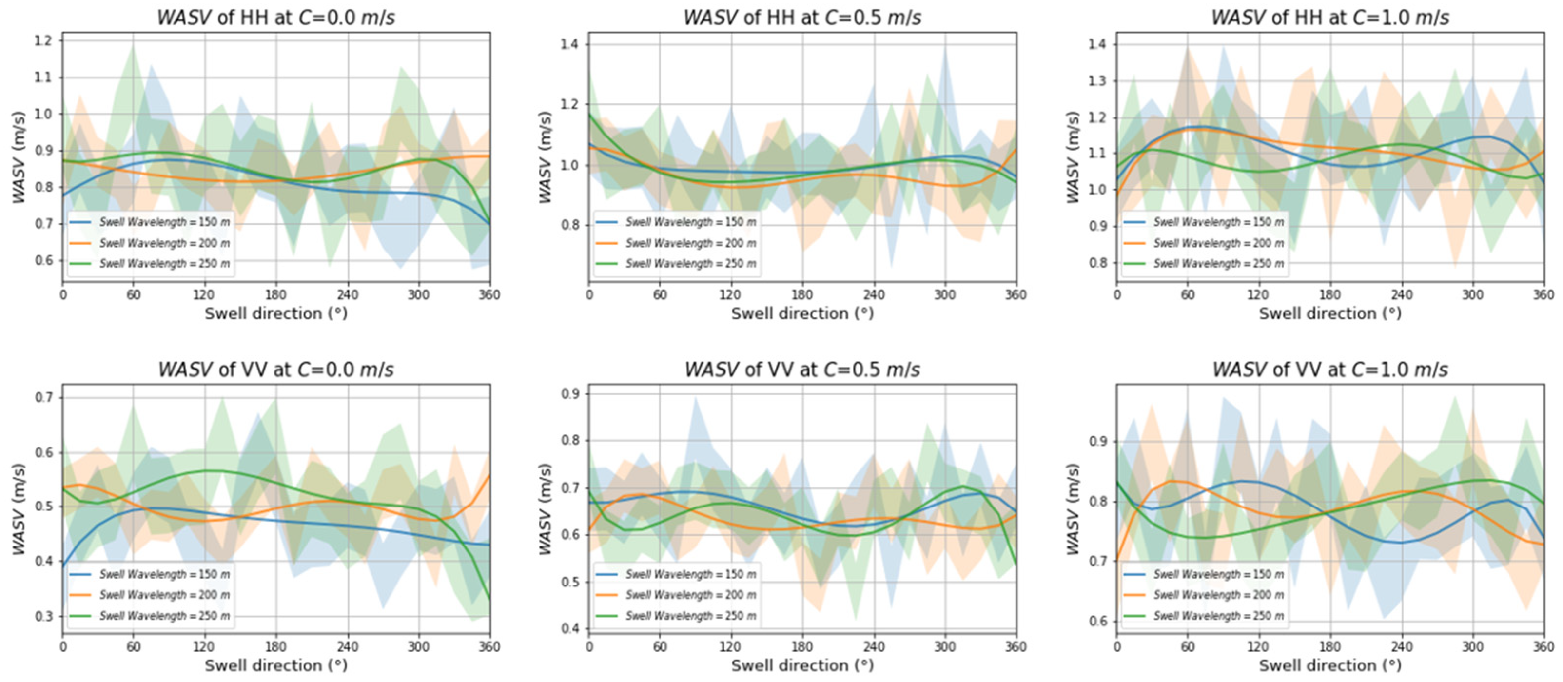
3.2.2. Swell Effect
4. Discussion
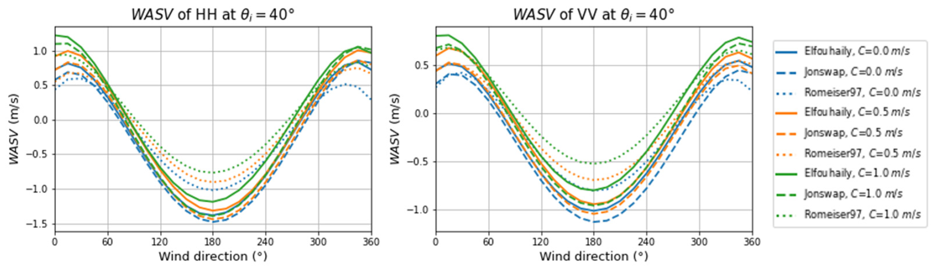
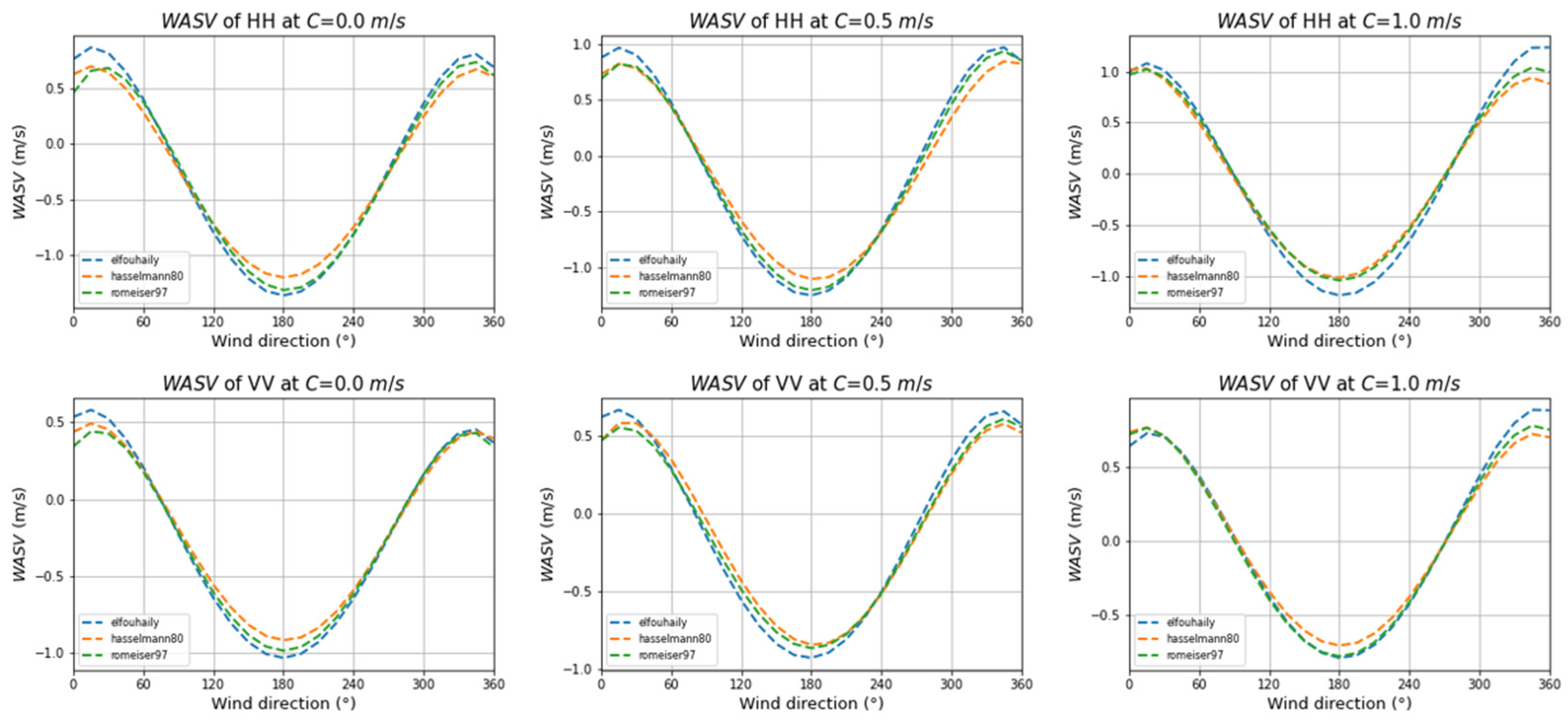
4.1. Influence of Wave Spectrum Models on WASV
4.2. Influence of Spreading Functions on WASV
5. Conclusions
Author Contributions
Funding
Conflicts of Interest
References
- Huang, W.; Carrasco, R.; Shen, C.; Gill, E.W.; Horstmann, J. Surface Current Measurements Using X-Band Marine Radar with Vertical Polarization. IEEE Trans Geosci Remote Sens. 2016, 54, 2988–2997. [Google Scholar] [CrossRef]
- Morang, A.; Gorman, L.T. Monitoring Coastal Geomorphology. In Encyclopedia of Coastal Science; Schwartz, M.L., Ed.; Springer: Dordrecht, The Netherlands, 2005; pp. 663–674. [Google Scholar]
- Feng, H.; Vandemark, D.; Levin, J.; Wilkin, J. Examining the Accuracy of GlobCurrent Upper Ocean Velocity Data Products on the Northwestern Atlantic Shelf. Remote Sens. 2018, 10, 1205. [Google Scholar] [CrossRef]
- Prandle, D.; Ryder, D.K. Measurement of surface currents in Liverpool Bay by high-frequency radar. Nature 1985, 315, 128–131. [Google Scholar] [CrossRef]
- Hammond, T.M.; Pattiaratchi, C.B.; Eccles, D.; Osborne, M.J.; Nash, L.A.; Collins, M.B. Ocean surface current radar (OSCR) vector measurements on the inner continental shelf. CSR 1987, 7, 411–431. [Google Scholar] [CrossRef]
- Quilfen, Y.; Chapron, B. Ocean Surface Wave-Current Signatures from Satellite Altimeter Measurements. Geophys. Res. Lett. 2019, 46, 253–261. [Google Scholar] [CrossRef]
- Bao, Q.; Lin, M.; Zhang, Y.; Dong, X.; Lang, S.; Gong, P. Ocean Surface Current Inversion Method for a Doppler Scatterometer. IEEE Trans. Geosci. Remote Sens. 2017, 55, 6505–6516. [Google Scholar] [CrossRef]
- Wineteer, A.; Torres, H.; Rodriguez, E. On the Surface Current Measurement Capabilities of Spaceborne Doppler Scatterometry. Geophys. Res. Lett. 2020, 47, e2020GL090116. [Google Scholar] [CrossRef]
- González-Haro, C.; Isern-Fontanet, J.; Tandeo, P.; Garello, R. Ocean Surface Currents Reconstruction: Spectral Characterization of the Transfer Function Between SST and SSH. J. Geophys. Res. Oceans 2020, 125, e2019JC015958. [Google Scholar] [CrossRef]
- Isern-Fontanet, J.; García-Ladona, E.; González-Haro, C.; Turiel, A.; Rosell-Fieschi, M.; Company, J.B.; Padial, A. High-Resolution Ocean Currents from Sea Surface Temperature Observations: The Catalan Sea (Western Mediterranean). Remote Sens. 2021, 13, 3635. [Google Scholar] [CrossRef]
- Goldstein, R.M.; Zebker, H.A. Interferometric radar measurement of ocean surface currents. Nature 1987, 328, 707–709. [Google Scholar] [CrossRef]
- Hansen, M.W.; Collard, F.; Dagestad, K.; Johannessen, J.A.; Fabry, P.; Chapron, B. Retrieval of Sea Surface Range Velocities From Envisat ASAR Doppler Centroid Measurements. IEEE Trans. Geosci. Remote Sens. 2011, 49, 3582–3592. [Google Scholar] [CrossRef]
- Romeiser, R.; Suchandt, S.; Runge, H.; Steinbrecher, U.; Grunler, S. First Analysis of TerraSAR-X Along-Track InSAR-Derived Current Fields. IEEE Trans. Geosci. Remote Sens. 2010, 48, 820–829. [Google Scholar] [CrossRef]
- Martin, A.C.H.; Gommenginger, C.P.; Jacob, B.; Staneva, J. First multi-year assessment of Sentinel-1 radial velocity products using HF radar currents in a coastal environment. Remote Sens. Environ. 2022, 268, 112758. [Google Scholar] [CrossRef]
- Mouche, A.; Collard, F.; Chapron, B.; Dagestad, K.-F.; Guitton, G.; Johannessen, J.; Kerbaol, V.; Hansen, M. On the Use of Doppler Shift for Sea Surface Wind Retrieval From SAR. IEEE Trans. Geosci. Remote Sens. 2012, 50, 2901–2909. [Google Scholar] [CrossRef]
- Martin, A.C.H.; Gommenginger, C.; Marquez, J.; Doody, S.; Navarro, V.; Buck, C. Wind-wave-induced velocity in ATI SAR ocean surface currents: First experimental evidence from an airborne campaign. J. Geophys. Res. Ocean. 2016, 121, 1640–1653. [Google Scholar] [CrossRef]
- Li, S.; Liu, B.; Shen, H.; Hou, Y.; Perrie, W. Wind Wave Effects on Remote Sensing of Sea Surface Currents From SAR. J. Geophys. Res. Ocean. 2020, 125, e2020JC016166. [Google Scholar] [CrossRef]
- Ardhuin, F.; Aksenov, Y.; Benetazzo, A.; Bertino, L.; Brandt, P.; Caubet, E.; Chapron, B.; Collard, F.; Cravatte, S.; Delouis, J.-M.; et al. Measuring currents, ice drift, and waves from space: The Sea Surface KInematics Multiscale monitoring (SKIM) concept. Ocean Sci. 2018, 14, 337–354. [Google Scholar] [CrossRef]
- Romeiser, R.; Runge, H.; Suchandt, S.; Kahle, R.; Rossi, C.; Bell, P. Quality Assessment of Surface Current Fields From TerraSAR-X and TanDEM-X Along-Track Interferometry and Doppler Centroid Analysis. IEEE Trans. Geosci. Remote Sens. 2013, 52, 2759–2772. [Google Scholar] [CrossRef]
- Ferreira, R.M.; Estefen, S.F.; Romeiser, R. Under What Conditions SAR Along-Track Interferometry is Suitable for Assessment of Tidal Energy Resource. IEEE J. Sel. Top. Appl. Earth Obs. Remote Sens. 2016, 9, 5011–5022. [Google Scholar] [CrossRef]
- Romeiser, R.; Thompson, D.R. Numerical study on the along-track interferometric radar imaging mechanism of oceanic surface currents. IEEE Trans. Geosci. Remote Sens. 2000, 38, 446–458. [Google Scholar] [CrossRef]
- Martin, A.C.H.; Gommenginger, C.P.; Quilfen, Y. Simultaneous ocean surface current and wind vectors retrieval with squinted SAR interferometry: Geophysical inversion and performance assessment. Remote Sens. Environ. 2018, 216, 798–808. [Google Scholar] [CrossRef]
- Yuan, X.; Lin, M.; Han, B.; Zhao, L.; Wang, W.; Sun, J.; Wang, W. Observing Sea Surface Current by Gaofen-3 Satellite Along-Track Interferometric SAR Experimental Mode. IEEE J. Sel. Top. Appl. Earth Obs. Remote Sens. 2021, 14, 7762–7770. [Google Scholar] [CrossRef]
- Scientific Assessment of TSCV Retrieval from Stereo-SAR: A critical Review. Available online: https://norceresearch.brage.unit.no/norceresearch-xmlui/bitstream/handle/11250/2649700/Norut_rapport_4-2018.pdf?sequence=1 (accessed on 16 March 2018).
- Stratton, J.A. Plane Waves in Unbounded, Isotropic Media. In Electromagnetic Theory; Wiley-IEEE Press: Hoboken, NJ, USA, 2015; pp. 268–348. [Google Scholar]
- Kudryavtsev, V.; Hauser, D.; Caudal, G.; Chapron, B. A semiempirical model of the normalized radar cross-section of the sea surface 1. Background model. J. Geophys. Res. Ocean. 2003, 108, FET 2-1–FET 2-24. [Google Scholar] [CrossRef]
- Romeiser, R.; Alpers, W.; Wismann, V. An improved composite surface model for the radar backscattering cross section of the ocean surface: 1. Theory of the model and optimization/validation by scatterometer data. J. Geophys. Res. Ocean. 1997, 102, 25237–25250. [Google Scholar] [CrossRef]
- Romeiser, R.; Alpers, W. An improved composite surface model for the radar backscattering cross section of the ocean surface: 2. Model response to surface roughness variations and the radar imaging of underwater bottom topography. J. Geophys. Res. Ocean. 1997, 102, 25251–25267. [Google Scholar] [CrossRef]
- Raney, R.K.; Runge, H.; Bamler, R.; Cumming, I.G.; Wong, F.H. Precision SAR processing using chirp scaling. IEEE Trans. Geosci. Remote Sens. 1994, 32, 786–799. [Google Scholar] [CrossRef]
- Yoshida, T.; Rheem, C.-K. Time-Domain Simulation of Along-Track Interferometric SAR for Moving Ocean Surfaces. Sensors 2015, 15, 13644–13659. [Google Scholar] [CrossRef]
- Stuhlmeier, R. Gerstner’s Water Wave and Mass Transport. J. Math. Fluid Mech. 2015, 17, 761–767. [Google Scholar] [CrossRef]
- Ritchie, R.H.; Marusak, A.L. The surface plasmon dispersion relation for an electron gas. Surf. Sci. 1966, 4, 234–240. [Google Scholar] [CrossRef]
- Donelan, M.A.; Hamilton, J.; Hui, W.H.; Stewart, R.W. Directional spectra of wind-generated ocean waves. Philos. Trans. R. Soc. Lond. Ser. A Math. Phys. Sci. 1985, 315, 509–562. [Google Scholar]
- Hasselmann, K.; Barnett, T.; Bouws, E.; Carlson, H.; Cartwright, D.; Enke, K.; Ewing, J.; Gienapp, H.; Hasselmann, D.; Kruseman, P.; et al. Measurements of wind-wave growth and swell decay during the Joint North Sea Wave Project (JONSWAP). Deut. Hydrogr. Z. 1973, 8, 1–95. [Google Scholar]
- Kahma, K.K. A Study of the Growth of the Wave Spectrum with Fetch. J. Phys. Oceanogr. 1981, 11, 1503–1515. [Google Scholar] [CrossRef]
- Phillips, O.M. Spectral and statistical properties of the equilibrium range in wind-generated gravity waves. J. Fluid Mech. 1985, 156, 505–531. [Google Scholar] [CrossRef]
- Elfouhaily, T.; Chapron, B.; Katsaros, K.; Vandemark, D. A unified directional spectrum for long and short wind-driven waves. J. Geophys. Res. Ocean. 1997, 102, 15781–15796. [Google Scholar] [CrossRef]
- Durden, S.; Vesecky, J. A physical radar cross-section model for a wind-driven sea with swell. IEEE J. Ocean. Eng. 1985, 10, 445–451. [Google Scholar] [CrossRef]
- Kodis, R. A note on the theory of scattering from an irregular surface. IEEE Trans. Antennas Propag. 1966, 14, 77–82. [Google Scholar] [CrossRef]
- Clarizia, M.P.; Gommenginger, C.; Bisceglie, M.D.; Galdi, C.; Srokosz, M.A. Simulation of L-Band Bistatic Returns from the Ocean Surface: A Facet Approach with Application to Ocean GNSS Reflectometry. IEEE Trans. Geosci. Remote Sens. 2012, 50, 960–971. [Google Scholar] [CrossRef]
- Yoshida, T.; Rheem, C.-K. SAR Image Simulation in the Time Domain for Moving Ocean Surfaces. Sensors 2013, 13, 4450–4467. [Google Scholar] [CrossRef]
- Wollstadt, S.; López-Dekker, P.; Zan, F.D.; Younis, M. Design Principles and Considerations for Spaceborne ATI SAR-Based Observations of Ocean Surface Velocity Vectors. IEEE Trans. Geosci. Remote Sens. 2017, 55, 4500–4519. [Google Scholar] [CrossRef]
- Elyouncha, A.; Eriksson, L.E.B.; Romeiser, R.; Ulander, L.M.H. Measurements of Sea Surface Currents in the Baltic Sea Region Using Spaceborne Along-Track InSAR. IEEE Trans. Geosci. Remote Sens. 2019, 57, 8584–8599. [Google Scholar] [CrossRef]
- Caldarella, N.; Lopez-Dekker, P.; Prats-Iraola, P.; Nouguier, F.; Chapron, B.; Zonno, M.; Rodriguez-Cassola, M. Retrieval of Wind and Total Surface Current Vectors Using Experimental Bidirectional Along-Track Interferometric TanDEM-X Data. IEEE Trans. Geosci. Remote Sens. 2022, 60, 5223412. [Google Scholar] [CrossRef]
- Zheng, C.W.; Li, C.Y.; Pan, J. Propagation Route and Speed of Swell in the Indian Ocean. J. Geophys. Res. Ocean. 2018, 123, 8–21. [Google Scholar] [CrossRef]
- Bhowmick, S.; Kumar, R.; Chaudhuri, S.; Sarkar, A. Swell Propagation over Indian Ocean Region. Int. J. Ocean Clim. Syst. 2011, 2, 87–99. [Google Scholar] [CrossRef]
- Miao, Y.; Dong, X.; Bourassa, M.A.; Zhu, D. Effects of Ocean Wave Directional Spectra on Doppler Retrievals of Ocean Surface Current. IEEE Trans. Geosci. Remote Sens. 2022, 60, 4204812. [Google Scholar] [CrossRef]
- Hasselmann, K.; Sell, W.; Ross, D.B.; Müller, P. A Parametric Wave Prediction Model. J. Phys. Oceanogr. 1976, 6, 200–228. [Google Scholar] [CrossRef]
- Hasselmann, D.E.; Dunckel, M.; Ewing, J.A. Directional Wave Spectra Observed during JONSWAP 1973. J. Phys. Oceanogr. 1980, 10, 1264–1280. [Google Scholar] [CrossRef]


| Parameter | Value |
|---|---|
| Wind speed | 5.0–15.0 (m/s) |
| Wind direction | 0.0–360.0 (°) |
| Wind fetch | 500 (km) |
| Current speed | 0.0, 0.5, 1.0 (m/s) |
| Current direction | 0.0 (°) |
| Swell amplitude | 0.5, 1.0, 1.5 (m) |
| Swell direction | 0.0–360.0 (°) |
| Swell wavelength | 150, 200, 250 (m) |
| The angle of incidence | 40 (°) |
| Radar frequency | 5.4 (GHz) |
| Number of channels | 2 |
| Baseline | 15 (m) |
| Mowing width | 1024 (m) |
| Resolution | 1 (m) |
| Polarization | HH, VV |
| Radar platform height | 693 (km) |
| Noise equivalent backscatter | −30 (dB) |
Publisher’s Note: MDPI stays neutral with regard to jurisdictional claims in published maps and institutional affiliations. |
© 2022 by the authors. Licensee MDPI, Basel, Switzerland. This article is an open access article distributed under the terms and conditions of the Creative Commons Attribution (CC BY) license (https://creativecommons.org/licenses/by/4.0/).
Share and Cite
Zhang, R.; Zhang, J.; Zhang, X.; Cao, C.; Wang, X.; Gao, G.; Liu, G.; Bao, M. Influence of Radar Parameters and Sea State on Wind Wave-Induced Velocity in C-Band ATI SAR Ocean Surface Currents. Remote Sens. 2022, 14, 4135. https://doi.org/10.3390/rs14174135
Zhang R, Zhang J, Zhang X, Cao C, Wang X, Gao G, Liu G, Bao M. Influence of Radar Parameters and Sea State on Wind Wave-Induced Velocity in C-Band ATI SAR Ocean Surface Currents. Remote Sensing. 2022; 14(17):4135. https://doi.org/10.3390/rs14174135
Chicago/Turabian StyleZhang, Rui, Jie Zhang, Xi Zhang, Chenghui Cao, Xiaochen Wang, Gui Gao, Genwang Liu, and Meng Bao. 2022. "Influence of Radar Parameters and Sea State on Wind Wave-Induced Velocity in C-Band ATI SAR Ocean Surface Currents" Remote Sensing 14, no. 17: 4135. https://doi.org/10.3390/rs14174135