Oceanic Kármán Vortex Streets in the Luzon Strait in the Lee of Didicas Island from Multiple Satellite Missions

Abstract

The oceanic Kármán vortex street is an important hydrokinetic phenomenon caused by the unsteady separation of sea currents in the wake of an obstacle. This study quantitatively analyzed the characteristics of the small-scale vortex street of Didicas Island in the Luzon Strait based on multimission satellite data. Five groups of vortex streets were captured, and each group was observed by two satellite images within one hour. Based on the displacement and change in the vortex street within one hour, we found that the formation time of a single vortex is longer than 40 min. The vortex propagation speed behind the island is approximately 0.98 m s⁻¹ (ranging from 0.66–1.22 m s⁻¹). The incoming velocity was calculated using the vortex propagation speed and the aspect ratio based on a vortex propagation model, which ranges from 0.72 to 1.47 m s⁻¹ The incoming speed is 1.6–2.3 times the geostrophic speed extracted from AVISO data, implying that the contribution of non-geostrophic flow to the total flow field is comparable to that of geostrophic flow in this region.

1. Introduction

Laboratory-scale periodic vortex shedding has been studied for more than 100 years in the field of fluid dynamics [1,2,3,4]. The initial studies on vortex streets were mainly in the field of atmospheric research, including aerospace research and the safety of bridges and high-rise buildings [5,6,7]. Since the mid-20th century, scientists have found that atmospheric vortex streets can occur on the leeward side of islands or mountains with the development of remote sensing technology [8,9,10,11]. Satellites can help to clearly observe the shape of the air vortex street pattern.

When oceanic currents flow around an obstacle, such as an island, the wake on the leeward side of the obstacle will become an ocean vortex street under certain conditions [12,13]. Ocean vortex streets are important for turbulent transport and energy dissipation. The vortex streets downstream of the islands are characterized by a double row of counterrotating vortices arranged in a staggered configuration. The approximate scale ranges for vortex streets are 0.1–10 km horizontally, 0.01–1 km vertically, and hours to days temporally [14]. The vortex size and shedding frequency induced by islands vary in different regions. The maximum rotation radius of the vortex street on the leeward side of Babuyan Island is 4.7 km, with a shedding period of 10.8 h [15]. The vortex size on the leeward side of Green Island is approximately 5 km and the shedding period is 14.8 h [16]. The vortex train induced by Phú Quý Island in the South China Sea has an average diameter of 28.1 ± 13.8 km and a shedding period of 1.02 days [17]. The incoming current velocity increases when vortex trains are formed [18].

The mechanism that favors the formation of the vortex street is still under discussion. The formation of the vortex street depends on the hydrodynamic conditions and the size of the obstacle. Wind is reported as the key factor in the formation of vortex streets on the scale of tens of kilometers in some studies [19]. In some regions, small-scale eddies are reported to be generated by the relative movement speed between rotating mesoscale eddies and the western boundary current [20]. On some islands, the interaction between the oceanic flow and the islands is regarded as the main reason for the formation of vortex streets [18]. Some regions show very weak vortex streets in the wake water, and most of the vortex streets are cyclonic, probably because of the high ratio of the Rossby number to the Burger number ($B_u$) [21,22].

Vortex streets in the ocean can transport nutrients vertically from the middle and deep layers to the euphotic layer, leading to phytoplankton blooms. Enhanced phytoplankton biomass has often been reported to occur around oceanic islands. Horizontal and vertical transport through vortices near an island result in the redistribution of nutrients and phytoplankton. Previous literature has shown that when the Kuroshio passes small islands, such as Green Island, submesoscale eddies are formed and are associated with colder, saltier, and higher phytoplankton water (both in the vertical and horizontal direction) [16,23].

Ocean dynamic satellites are able to observe mesoscale processes, such as the current products from AVISO (Archiving, Validation and Interpretation of Satellite Oceanographic) and OSCAR (Ocean Surface Current Analysis Real-time); however, their spatial resolution (tens of kilometers) is not sufficient to observe vortices on the order of several kilometers or tens of kilometers. Optical and SAR (Synthetic Aperture Radar) satellite data can compensate for this deficiency to a certain extent [15,17,18,19,20]. These studies mainly focus on vortex streets in the order of tens of kilometers, whereas few studies have involved observations of vortices in the order of tens of meters to one kilometer as in the present study. Vortices on the order of less than one kilometer cannot be captured by optical satellites with spatial resolutions ranging from several hundred meters to several kilometers, such as GOCI (Geostationary Ocean Color Imager), SeaWiFS (Sea-viewing Wide Field-of-view Sensor), MODIS (Moderate Resolution Imaging Spectroradiometer), MERIS (Medium Resolution Imaging Spectrometer), and Sentinel-3 [20] but can be observed by satellites with spatial resolutions in the order of ten meters, such as Landsat, Sentinel-2, Haiyang-1C CZI (Coastal Zone Image), and Gaofen-1 (GF-1). However, a satellite with a higher spatial resolution usually has a longer revisit period (the time interval between two observations of the same area, e.g., 16 days in the case of Landsat). This prevents us from observing the variability of the dynamic processes of the vortex street. To overcome the above shortcomings, we applied multisatellite data to identify smaller-scale vortices and their dynamic variations within one hour. Multisatellite products with a high spatial resolution also provide a way to obtain the incoming current of vortex streets. The calculation of the incoming current of vortex streets is a challenging problem. Hsu et al. [16] used the maximum cross-correlation (MCC) method to calculate the incoming velocity based on the Himawari-8 SST images, which have a temporal resolution of 10 min and a spatial resolution of 2 km. Using in situ data and satellite data to observe vortex streets, they found an average incoming surface current speed of 1.15 m/s for Green Island. In the present study, we used multimission satellite remote sensing data with a spatial resolution of tens of meters to analyze the small-scale Kármán vortex streets on Didicas Island in the Luzon Strait. The aspect ratio and propagation velocity of vortex streets were estimated based on the multimission satellite data with an observation time interval of one hour. The incoming current velocity in front of the island was then calculated based on a vortex propagation model and the above parameters from the satellite data.

2. Materials and Methods

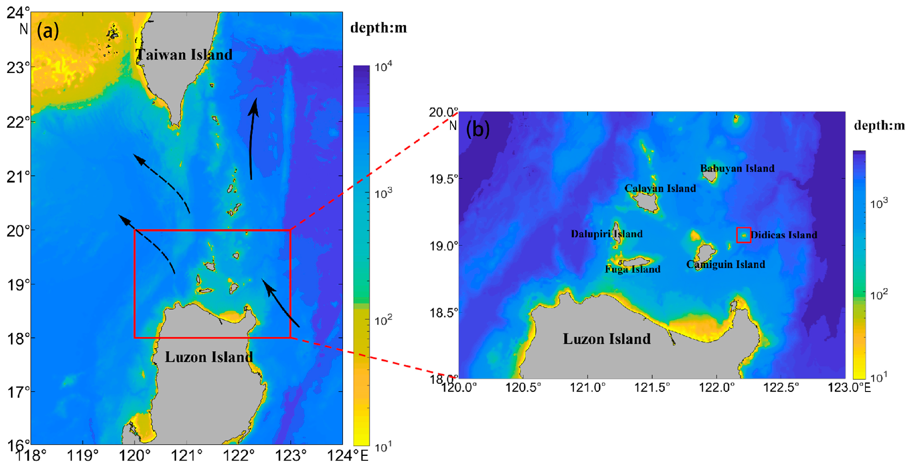
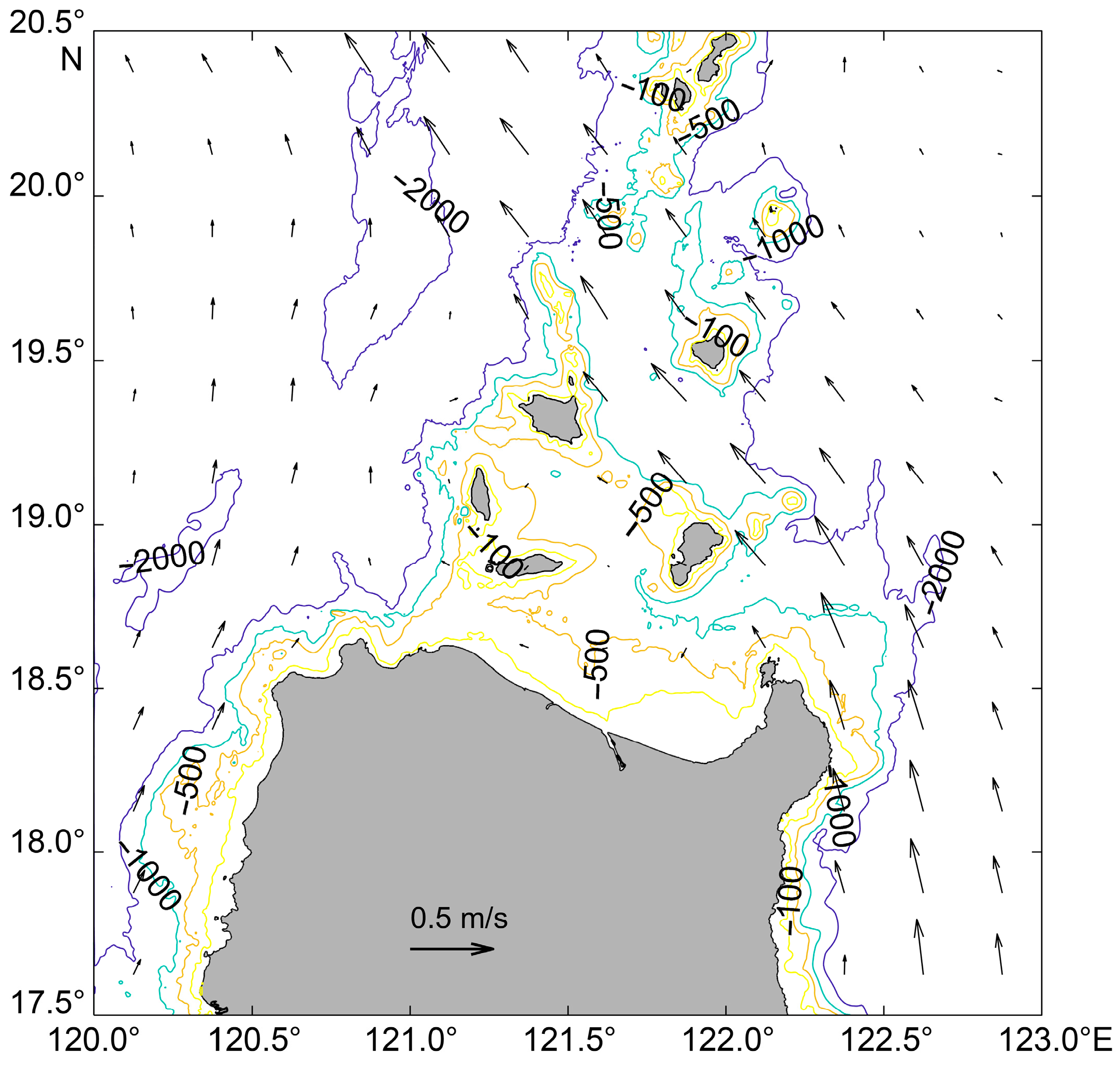
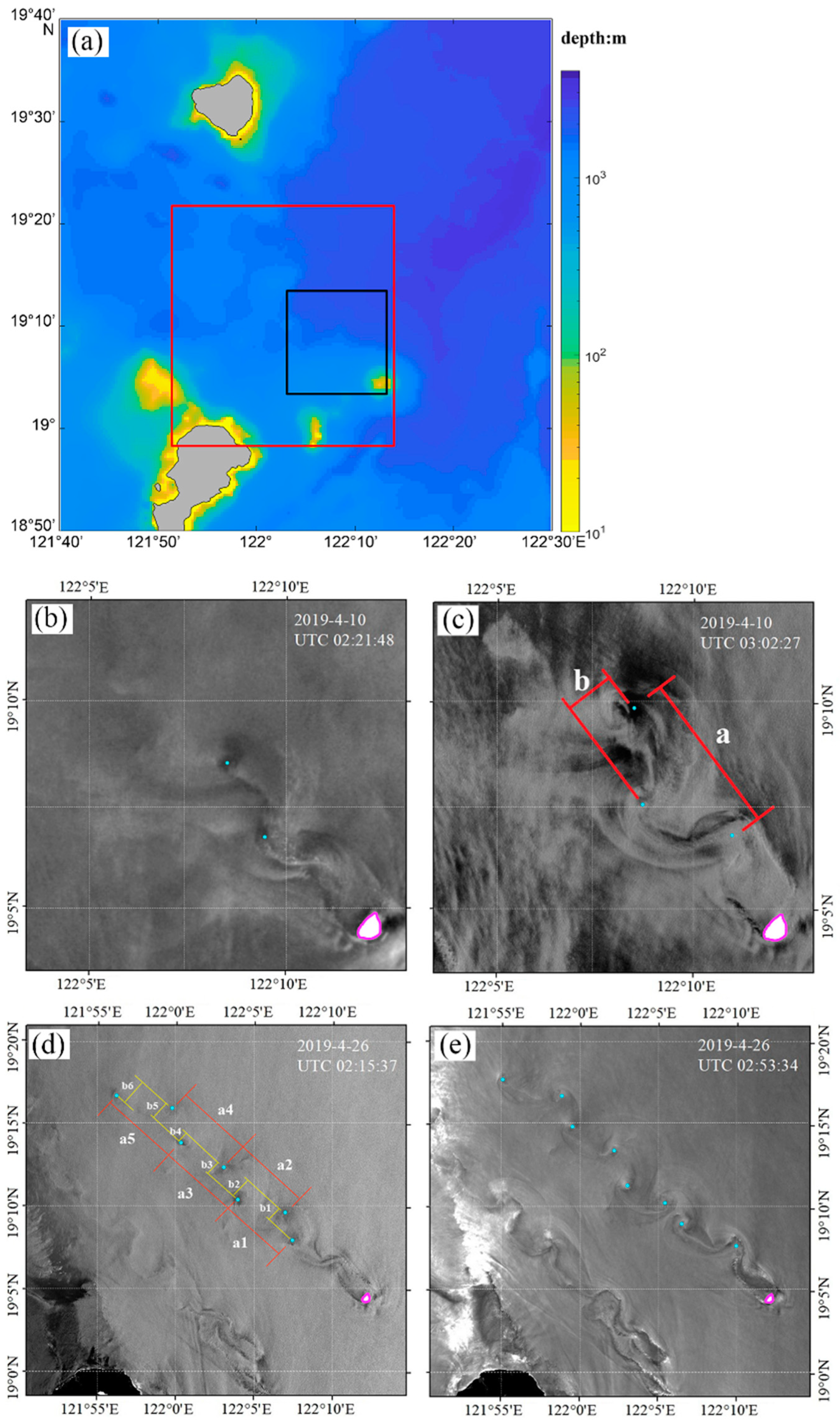
2.1. Study Area

The study area is located in the Luzon Strait (Figure 1). The Luzon Strait is the key channel for water exchange between the South China Sea and Northwest Pacific. The Kuroshio is a strong surface oceanic current of the western Pacific Ocean, and the northward flowing continuation of the Pacific North Equatorial Current between Luzon of the Philippines and the east coast of Japan. When passing by the Luzon Strait, a branch of the Kuroshio flows northwestward into the South China Sea (SCS). The Kuroshio transports tremendous amounts of heat, salt, and nutrients poleward and to the SCS from the Luzon Strait [24,25,26]. The Kuroshio intrusion to the SCS has a seasonal pattern and is stronger in winter than in summer [27]. The surface Kuroshio water can intrude deep into the SCS, especially in winter [28]. There are many islands in the Luzon Strait. The strong current, and the complex topography of the strait combine to create complicated ocean dynamic processes in the strait, and the small-scale processes are active.

Didicas Island, a member of the Babuyan Islands group, is located in the Luzon Strait (north of Luzon and south of the Batanes Islands, Figure 1). The midpoint longitude and latitude coordinates are 122.20°E and 19.07°N, respectively. The Kuroshio current is the strong northwestern component of the inflows near Didicas Island. The mean diameter of Didicas Island is approximately 1 km. The bathymetry map (Figure 2) shows that the underwater terrain around the island is steep, quickly descending to 1000 m. The complex underwater topography leads to the complex and changeable current in this area [16].

2.2. Satellite Data

In this study, multisatellite data were used to identify vortices. According to the scale of the vortex street in the area, we selected the following five satellite sensors: Landsat-8, Sentinel-2, GaoFen-6 (GF-6), GaoFen-1 (GF-1), and HY-1C CZI. Information on the spectral and spatial resolutions is shown in

Table 1. The parameters of the satellite data used in this research.

Satellite Sensors	Original Spatial Resolution(m)	Product Level	Bands in Visible Spectrum	Swath Width (km)	Scenes Without Clouds	Scenes with Kármán Vortex Street
Landsat-8	30	L1TP	9	185	12	5
Sentinel-2	10/20/60	L1C	13	290	38	4
GF-1/6 MSS	16	WFV	4/8	800	3	3
HY-1C CZI	50	L1C	4	950	4	4

Note: MSS (Multispectral Scanner System); CZI (Coastal Zone Image); L1TP (Level 1 Precision Terrain (Corrected)); L1C (Level-1C); WFV (wide field of view).

.

Landsat-8 Operational Land Imager (OLI) level-1 data were obtained from the U.S. Geological Survey. The Sentinel-2 Multispectral Imager (MSI) level-1 data used in this study were obtained from the European Space Agency. The GF-1 and GF-6 satellite data were obtained from the China Centre for Resources Satellite Data and Application. Both GF-1 and GF-6 are equipped with two multispectral scanners: one scanner has a 2-m resolution in the panchromatic band and an 8-m resolution in the multispectral bands, and the other scanner has a 16-m resolution in the multispectral bands. We used the data from the multispectral scanners with a 16-m resolution in this research. The 16-m multispectral scanner was designed at an observation field width of 800 km, with 4 bands in GF-1 and 8 bands in GF-6. HY-1C CZI data, with a spatial resolution of 50 m, were also used in this study. HY-1C data were distributed by the National Satellite Ocean Application Service, China.

Landsat-8, Sentinel-2, and HY-1C data were used to find the days with Kármán vortex streets as our main data. The blue band data were used as grayscale figures to determine whether a vortex street existed in the study region. Then, we focused on these days and tried to find images from other satellites such as GF-1 and GF-6. Satellite data from January 2018 to August 2020 were used.

All the calculations were based on geo-corrected satellite data. Landsat-8, Sentinel-2, and HY-1C products were geometrically corrected by the distributor. GF-1/6 data were geometrically corrected with the Environment for Visualizing Images (ENVI). With its geometric correction tool, GF-1/6 data were corrected with their own Rational Polynomial Coefficient (RPC) information. In this study, vortex streets on the same day from two different satellites were compared for analysis. Therefore, satellite data were resampled to the lower spatial resolution of the two images. For instance, when comparing the GF-6 image with the HY-1C image, the GF-6 data were resampled to 50 m × 50 m.

Surface current velocity data were obtained from AVISO with a spatial resolution of 0.25° × 0.25° (product ID: SEALEVEL_GLO_PHY_L4_MY_008_047, DOI: https://doi.org/10.48670/moi-00148). The product is generated by the processing system, including data from all altimeter Copernicus missions (Sentinel-6A, Sentinel-3A/B) and other collaborative or opportunity missions (e.g., Jason-3, Saral/AltiKa, Cryosat-2, OSTM/Jason2(Ocean Surface Topography Mission/Jason-2), Jason-1, Topex/Poseidon, Envisat (Environmental Satellite), GFO (GEOSAT Follow-On), ERS-1/2 (European Space Agency-1/2), HY-2A/B).

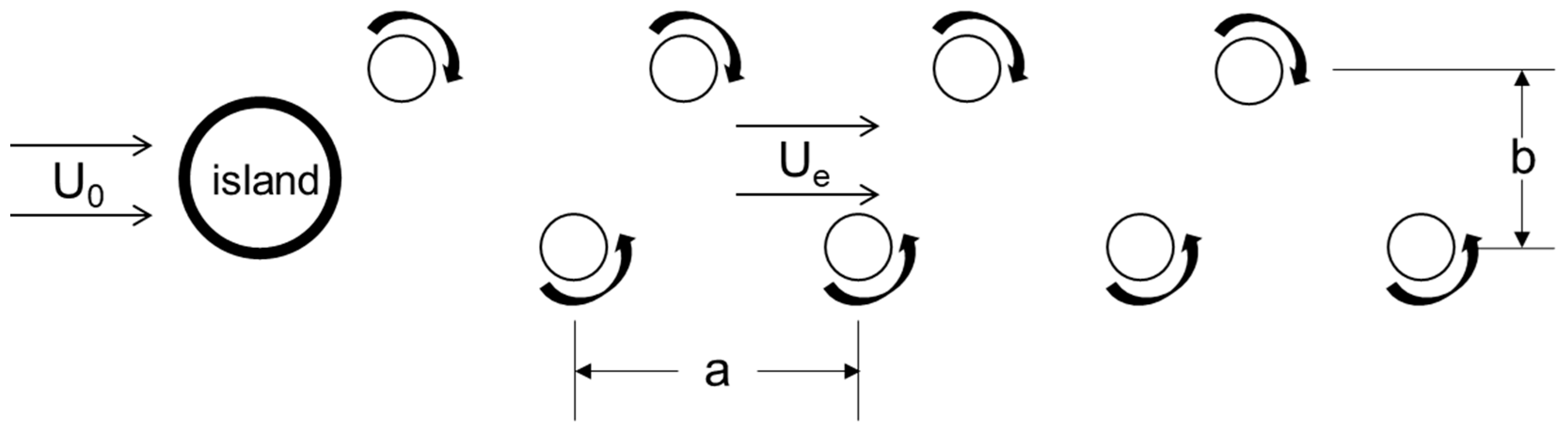
2.3. Property Parameters of Vortex Streets

Figure 3 shows the diagram of the vortex street, and $U_0$ is the incoming flow speed. A vortex street consists of two rows of vortices, which have opposite rotating directions. The vortices are staggered such that a vortex in one row lies opposite the center of the downstream spacing a between adjacent vortices in the other row [29,30]. In this research, the aspect ratio Ar was calculated as a/b, where a and b represent the longitudinal spacing in one row and transverse spacing between two rows, respectively, as shown in Figure 3.

The ratio b/a = 0.281 (also 1/Ar) was used for neutrally stable dimensions, which means that Kármán vortex streets will always exist stably. This ratio is dependent on the shape of the obstacle, the characteristics of the flow, and the distance along the wake and was observed in laboratory investigations to lie within the range of 0.28 < b/a < 0.52 [8,9].

In our study area, the scale of the Kármán vortex street is quite small (approximately 1 km); thus, the incoming current velocity $U_0$ cannot be calculated with the method used by Hsu et al. [16] due to the low resolution. Another method to calculate $U_0$ is introduced.

Vortex propagation was represented as the model given by Tsuchiya in earlier research [31] as Equation (1):

$$\left(2B-A\right)X^2+\left(2A-3B\right)X+B-A+B/\left(4A\right)=0$$

(1)

where $X=U_e/U_0$, $A=coth\left(\pi \times b/a\right)$, $B=\pi \times b/a$, and $U_e$ is the vortex propagation velocity.

b/a can be substituted into Equation (1) to obtain $U_e/U_0$, in which, $U_e$ can be measured from consecutive remote sensing images. The same Kármán vortex street is observed with different satellite images and the displacement of the vortices is measured. Based on the displacement and the time interval of two satellite images, the propagation velocity of vortices $U_e$ is calculated. Then, $U_0$ can be estimated based on the obtained $U_e$ and $U_e/U_0$.

In a nonrotating unstratified fluid, the vortex feature is determined by the Reynolds number, Re. The Reynolds number is the dimensionless ratio of inertial force to viscous force (Equation (2)) and is calculated as follows:

$$Re=\frac{U_{0}D}{\nu }$$

(2)

where $D$ is the crosscurrent island diameter (1.1 km in this study), and ν is the horizontal eddy diffusivity, which was set as 10 ${\mathrm{m}}^2 {\mathrm{s}}^{-1}$ [15].

In the study of rotating fluids, one more dimensionless dynamical parameter should be introduced, which is usually the Rossby number. The Rossby number is the ratio of inertial force to Coriolis force, defined as follows:

$$Ro=\frac{U_0}{fD}=\frac{U_0}{2D\mathsf{\Omega }sin\phi }$$

(3)

where $f=2\mathsf{\Omega }sin\phi$ is the Coriolis parameter, with $\mathsf{\Omega }=7.29\times {10}^{-5}{\mathrm{s}}^{-1}$ being the rate of the Earth’s rotation and $\phi$ = 19.075° being the latitude of our target.

To consider ocean stratification, the dimensionless Burger number is often used. It is defined as the ratio between the density stratification in the vertical direction and the Earth’s rotation in the horizontal direction:

$$Bu=\frac{R_D}{R}$$

(4)

where $R$ is the radius of the island $\left(2R=\mathrm{D}\right)$; $R_D=Nh/f$ is the Rossby deformation radius, in which $h$ is the typical depth of the upstream current; and $N=\sqrt{\frac{g}{{\rho }_0}\frac{\partial \rho }{\partial z}}$ is the Brunt–Väisälä parameter, where g is the acceleration due to gravity and ${\rho }_0$ is the reference density of the ocean.

Although it is not a control parameter, the Strouhal number is an essential dimensionless quantity in the description of oscillating flows. At high Strouhal numbers, oscillations dominate the flow while at low Strouhal numbers, the oscillations are swept by the fast-moving fluid. It can be considered a normalized shedding frequency, defined as follows:

$$St=\frac{D}{TU}$$

(5)

where $T$ is the shedding period between two consecutive vortices in the same row. Here, $T=a/U_e$, where a is the longitudinal spacing in one row and $U_e$ is the vortex propagation velocity.

2.4. Chlorophyll-a Retrieval

The Landsat-8 OLI chlorophyll-a concentration was derived using the SeaDAS processor (version 7.5, provided by NASA in Washington, MA, USA). The aerosol removal of Landsat-8 uses band ratios of the combination of OLI bands 5 and 7. The chlorophyll-a retrieval algorithm uses the 443, 561, and 655 nm bands for the band difference and the 443, 482, and 561 nm bands for the band ratio. In low-chlorophyll water, in which chlorophyll-a ≤ 0.25 mg m⁻³, the chlorophyll-a concentration is retrieved with the three-band difference color index (CI) [32] method, as shown in Equations (6) and (7). In high-chlorophyll water, in which chlorophyll-a ≥ 0.30 mg m⁻³, the chlorophyll-a concentration is retrieved with the method of the traditional band ratio algorithm (OC3), as shown in Equations (8) and (9). Intermediate-chlorophyll waters in the transition zone of 0.25–0.3 mg m⁻³ were retrieved with a weighted mixture of the two algorithms, as shown in Equation (10). Collectively, the algorithm is termed the Ocean Color Index (OCI) algorithm. The empirical coefficients were adjusted for OLI using the NASA Bio-Optical Marine Algorithm Dataset [33]:

$$CI=R_{rs561}-\frac{R_{rs443}+\left(561-443\right)}{\left(655-443\right)\times \left(R_{rs655}-R_{rs443}\right)}$$

(6)

$$lo{g}_{10}\left(CH{L}_{CI}\right)=a\times CI+b$$

(7)

where $R_{rs} \mathrm{is}$ the remote sensing reflectance, the number subscript is the central wavelength from the satellite, and $CH{L}_{CI}$ is the chlorophyll-a concentration retrieved with the CI method. a and b are the CI algorithm coefficients from the NASA Bio-Optical Marine Algorithm Dataset:

$$X=lo{g}_{10}\left(\frac{\max \left(R_{rs443 },R_{rs482}\right)}{R_{rs561}}\right)$$

(8)

$$lo{g}_{10}\left(CH{L}_{OC3}\right)=a_0+a_1\times X+a_2\times X^2+a_3\times X^3+a_4\times X^4$$

(9)

where $a_0,a_1,a_2,a_3,a_4$ are the algorithm coefficients, and $\max \left(R_{rs443},R_{rs482}\right)$ is the maximum $R_{rs}$ of two:

$$CHL=\alpha \times CH{L}_{CI}+\beta \times CH{L}_{OC3}$$

(10)

where the weighting factors are $\alpha =\frac{CH{L}_{CI}-0.25}{0.3-0.25}$, $\mathrm{and}\beta =\frac{0.3-CH{L}_{CI}}{0.3-0.25}$.

3. Results

3.1. Probability of Occurrence of the Kármán Vortex Street

To investigate the pattern and evolution of the vortex street, daily satellite images from January 2018 to August 2020 were used to identify the vortex streets. Excluding satellite imagery with cloud coverage, 55 days of cloudless images were acquired, mainly in summer and autumn. Among the 55 days, the Kármán vortex street was observed on 11 days, indicating an empirical probability of 1/5. The Kármán vortex street mainly occurs from April to July, with more frequent occurrences in April and May (

Table 2. The cloud-free days in the study area in different months and the visible Kármán vortex street days.

Month	Jan.	Feb.	Mar.	Apr.	May.	Jun.	Jul.	Aug.	Sep.	Oct.	Nov.	Dec.
Days of Data without Clouds	2	4	6	8	9	9	5	2	3	4	1	2
Days of Data with Kármán Vortex Street	0	0	0	3	5	1	2	0	0	0	0	0

). Among these vortex streets, five groups of vortex streets were captured by two satellite images with a time interval of approximately 30–40 min.

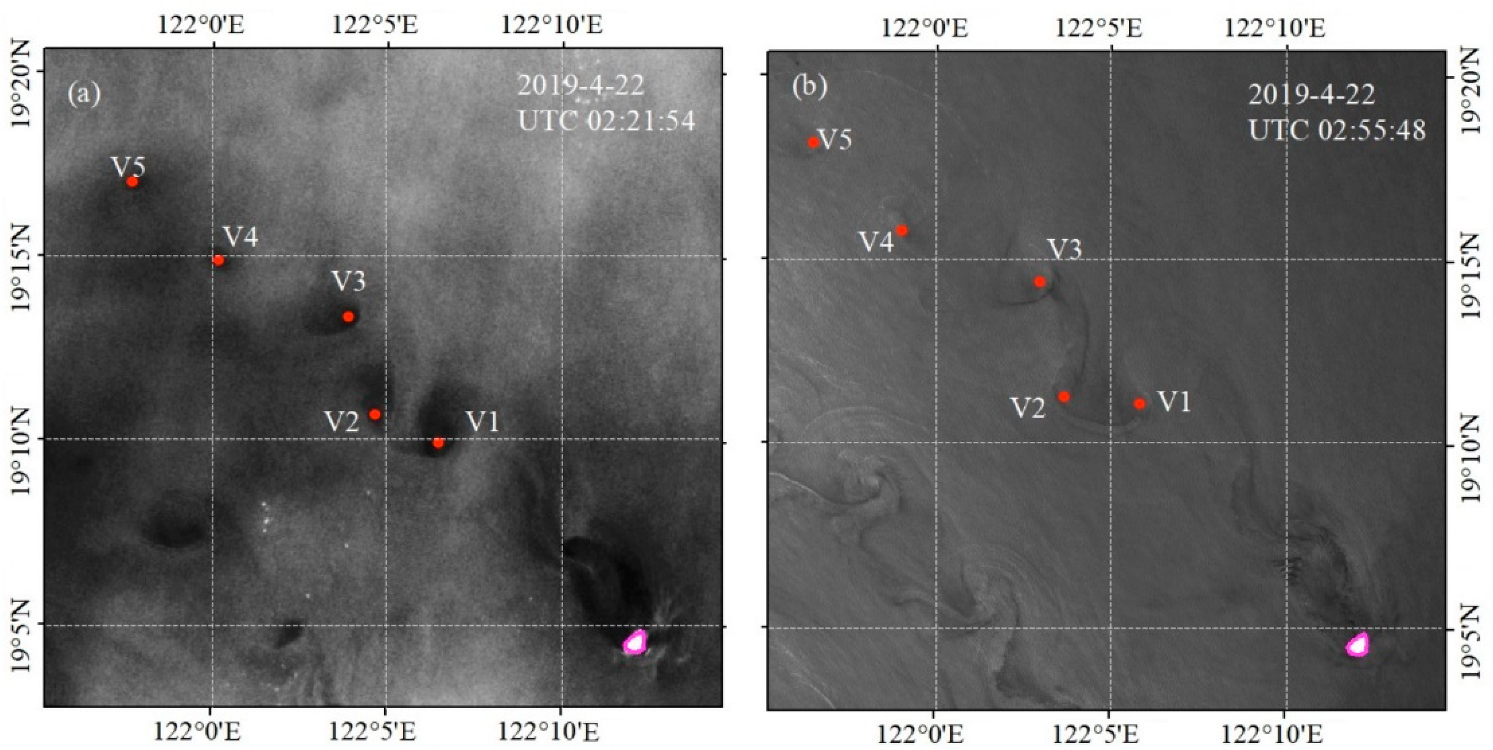
3.2. Distribution Pattern of the Kármán Vortex Street

The northwestward flow of the Kuroshio passes Didicas Island and tends to generate a repeating pattern of counterrotating vortex pairs. Figure 4 shows two groups of vortex streets, which are observed by two satellites. The first group, as shown in Figure 4b,c, was acquired on UTC 02:21:48 and UTC 03:02:27 of 10 April 2019, from the HY-1C CZI and GF-6 satellites, respectively, with an observation time interval of 41 min. The wake on the leeward side of the island occurred at UTC 2:21:48, at which no obvious rotating vortices were observed (Figure 4b). In 41 min, the vortices formed and strengthened (Figure 4c), and an anticyclonic and a cyclonic vortex can be clearly observed. The vortex presents a pattern of light and dark in the satellite image, and the center of the darkest area in the vortex is defined as the vortex center in this study, which is used as a reference point to track the moving distance of the vortex. Compared with the island wake in Figure 4b, there is an increase in both the distance between the two rows of vortices b and the distance between two consecutive vortices a in Figure 4c. It is estimated that a = 6.918 km, b = 2.687 km, and the aspect ratio Ar is 2.575. Furthermore, the diameter of the vortices increases.

A vortex street composed of multiple vortices is shown in Figure 4d,e (the second group of vortex streets), which were obtained on UTC 02:15:37 and UTC 02:53:34 of 26 April 2019, from the Landsat-8 and GF-6 images, respectively (with a time interval of approximately 38 min). In Figure 4d, a recirculation flow develops behind the island followed by a wave-like tail. The entire wave resembles a weak vortex street. Seven vortices and one unformed vortex are presented first. After 38 min, the unformed vortex takes form, and eight vortices in total were observed, as shown in Figure 4e, indicating that the vortex formation period is longer than 38 min. The mean distance between two rows of vortices b and the mean distance between two consecutive vortices a are 1.653 and 8.646 km, respectively. The aspect ratio $Ar$ is 5.23.

Figure 4 shows that almost all vortex streets are northwest trending. Horizontal length scales are similar to the island diameter. The number of vortices in a group of vortex streets can reach eight. The vortex streets are uniformly symmetrical or diffusely symmetrical. The signals of cyclonic and anticyclonic vortices are equally obvious, which is different from the eastward transported vortex street (obvious asymmetry in cyclone and anticyclone signals).

As mentioned in Section 3.1, five vortex streets were captured by two satellite images.

Table 3. Vortex street patterns identified by different satellites. Br = mb/D.

Date	Satellite	Vortices	$\mathit{a}$ (km)	$\mathit{b}$ (km)	$\mathit{A}\mathit{r}$	$\mathit{B}\mathit{r}$
10 April 2019	HY-1C	2	/	1.059	/	0.963
	GF-6	3	6.918	2.687	2.577	2.442
22 April 2019	HY-1C	5	9.197	2.113	4.348	1.921
	GF-6	5	9.568	2.641	3.623	2.401
26 April 2019	Landsat-8	7	8.497	1.876	4.525	1.705
	GF-6	8	8.646	1.653	5.236	1.502
27 May 2020	Sentinel-2	5	8.407	1.206	6.993	1.096
	HY-1C	5	8.449	1.240	6.803	1.127
30 May 2020	Landsat-8	4	9.164	2.055	4.464	1.868
	HY-1C	5	8.061	2.254	3.571	2.049

gives the statistical results of the distribution characteristics for all five groups of vortex streets. The average a and b are approximately 8.5 and 1.8 km, respectively. The calculated mean aspect ratio Ar is 4.17. The theoretical value of the ratio 1/Ar in an inviscid fluid was 0.281 in earlier studies, which was thought to be neutrally stable [34,35]. However, the actual ratio varies from a value smaller than 0.2 and a value greater than 0.4 due to turbulent diffusion, and it was found to have a slight dependence on Re [36]. Our results do not show significant dependences of the aspect ratio on Re.

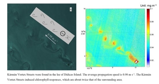
3.3. Propagation Characteristics

Based on the observations of the multimission satellite on the same set of vortex streets, the vortex propagation velocity $U_e$ can be estimated based on the movement distance and interval time by comparing two consecutive satellite observations. Due to the short time interval, it is easy to identify the same vortices between two satellite images. Figure 5 shows a case for the calculation of $U_e$. The same Kármán vortex street was observed by HY-1C CZI and GF-6 with a time interval of 34 min, as shown in Figure 5. All the centers of vorticities, from V1 to V5, show a displacement in the northwest direction within 34 min. Measuring the distance of each vortex reveals that the average propagation distance is 2.49 km, and thus, the propagation velocity $U_e$ is 1.22 m s⁻¹ (dividing the distance by the time interval). Then, by substituting each ratio 1/Ar (also b/a) into Equation (1), $U_e/U_0$ is obtained, ranging from 0.78 to 0.92. Based on the obtained $U_e/U_0$ and the propagation velocity $U_e$, the incoming flow speeds $U_0$ are calculated.

Table 4. The fluid speed of the Kármán vortex street and fluid parameters.

Date	Distance (km)	${\mathit{U}}_{\mathit{e}}$ (m s−1)	${\mathit{U}}_0$ (m s−1)	${\mathit{U}}_{\mathit{e}}/{\mathit{U}}_0$	$\mathit{T}$	$\mathit{R}\mathit{e}$	$\mathit{S}\mathit{t}$	$\mathit{R}\mathit{o}$
10 April 2019	2.23	0.91	1.17	0.78	2.12	129	0.123	22.30
22 April 2019	2.49	1.22	1.47	0.83	2.13	162	0.098	28.10
26 April 2019	2.52	1.11	1.28	0.87	2.15	140	0.111	24.37
27 May 2020	1.55	0.66	0.72	0.92	3.54	79	0.120	13.78
30 May 2020	2.36	0.99	1.19	0.83	2.41	131	0.106	22.79

shows the fluid speed of the Kármán vortex street and the related parameters for the five observed vortex streets. The incoming flow speed ranges from 0.72 to 1.47 m s⁻¹. The vortex propagation speed downcurrent of the island is slower than the incoming flow speed, ranging from 0.66 to 1.22 m s⁻¹. It increases as the inflow velocity increases. The $Re$ and Ro values range from 79 to 162 and from 13.78 to 28.10, respectively. These values increase with the incoming flow speed according to their definition.

The shedding period is approximately 2–3 h. It should be noted that the shedding period of the vortex here is different from the minimum time required to form a vortex obtained by satellite observations, as described above. The vortex shedding period can be understood as the time interval between the beginning of the formation of two adjacent vortices in the same row, which includes the formation, shedding, and propagation of the vortex, until the next vortex in the same row begins to form. Its calculation formula $T=a/U_e$ in the description of Equation (5) helps to understand this concept.

Compared with the geostrophic velocity observed by the altimeter (

Table 5. Comparison of our estimated flow velocity with AVISO observations. $U_0$__aviso and $U_e$_{_aviso} are the flow velocities in front and on the leeward side of the island, respectively, which were obtained from AVISO. Angle indicates the flow direction, and the geographical east was defined as 0°. The biases of $U_e$ and $U_e$_{_aviso} were calculated.

Date	${\mathit{U}}_{\mathit{e}\mathbf{\_}\mathbf{aviso}}$ (m s−1)	${\mathit{U}}_{\mathit{e}}/{\mathit{U}}_{\mathit{e}\mathbf{\_}\mathbf{aviso}}$	${\mathit{U}}_{\mathit{e}\mathbf{\_}\mathbf{aviso}}$ (m s−1)	${\mathit{U}}_{\mathit{0}}/{\mathit{U}}_{\mathit{e}\mathbf{\_}\mathbf{aviso}}$	Angle ${\mathit{U}}_{\mathit{e}}$ (°)	Angle ${\mathit{U}}_{\mathit{e}\mathbf{\_}\mathbf{aviso}}$ (°)	Angle Bias (°)
10 April 2019	0.73	1.3	0.66	1.8	131.3	119.7	11.6
22 April 2019	0.77	1.6	0.71	2.1	135.8	123.0	12.7
26 April 2019	0.82	1.4	0.71	1.8	139.7	132.3	7.5
27 May 2020	0.60	1.1	0.45	1.6	136.4	139.5	−3.2
30 May 2020	0.68	1.5	0.51	2.3	139.5	146.0	−6.6

, see the columns $U_0$/$U_0$__aviso), our estimated incoming flow speed is 1.6–2.3 times the current speed of the nearest AVISO data in the direction of the incoming flow. The contribution of non-geostrophic flow to the total flow field is comparable to that of geostrophic flow in this region. The direction deviation between our estimated vortex propagation direction and the AVISO data is from 3° to 13°. Comparing Re, Ro, and $U_0$/$U_0$__aviso, $U_e$/$U_e$__aviso and the angle bias reveals that the larger the Ro and Re numbers are, the greater the contribution of the non-geostrophic flow speed to the total flow speed; meanwhile, due to the impact of the non-geostrophic flow, the angle bias also increases. This also verifies the accuracy of our estimation of flow velocity using multimission satellite data.

4. Discussion

Quasi-symmetry of the cyclonic and anticyclonic vortices in our study area was observed. However, the asymmetry was less obvious than that in previous studies in other areas. This asymmetry is thought to be associated with the Earth’s rotation and the nonaxisymmetric shape of the island [37]. Centrifugal instability preferentially destroys cyclonic vortices, leaving a streak of anticyclones further downstream. A previous study revealed that in the small $Ro/Bu$ regime, cyclonic and anticyclonic eddies behaved symmetrically. In the large $Ro/Bu$ regime, the asymmetry depends on $Re$ when $Re$ is moderate or small, the anticyclonic vortex is dominant over the cyclone; when $Re$ is larger, a cyclonic vortex is dominant [21]. The phytoplankton footprint associated with the vortex street more clearly shows this quasi-symmetric characteristic of cyclonic and anticyclonic vortices. An increase in the chlorophyll concentration of the water leeward of the island is observed by Landsat-8 OLI with a 30 m spatial resolution, implying enhanced phytoplankton productivity caused by flow disturbance for both cyclonic and anticyclonic vortices (Figure 6). The maximum chlorophyll concentration in the vortex center is approximately twice that of the surrounding chlorophyll. Phytoplankton blooms associated with vortices can be observed at a large distance of approximately 37 km downstream from the island. The source water forming the vortices leeward of the island is characterized by a high level of chlorophyll. It seemed that the chlorophyll level inside the first vortex may be influenced by the chlorophyll of the source water forming the vortices (on the leeward side of the island). Then, the chlorophyll level increases at the second and third vortices, implying that there is nutrient supply and that it stimulates phytoplankton growth. Moreover, the bloom size also increases at the second and third vortices. Then, both the chlorophyll level and bloom size decrease from the fourth vortex.

The phytoplankton response to island-generated vortices depends on many factors, such as the phytoplankton level of the source water forming the vortices, the characteristics of the vortices (scale and lifespan, etc.), the response time of phytoplankton, and the interaction between cyclonic and anticyclonic vortices and the surrounding waters. The water around the study island is characterized as eutrophic. If the initial chlorophyll concentration is assumed to be approximately 0.05 mg m⁻³ at the first vortex location and chlorophyll growth is only affected by the nutrient supply, for phytoplankton growth rates of ~0.2 day⁻¹ [38] and a shedding period of ~3 h, the chlorophyll level at the first vortex should be approximately 0.0251 mg m⁻³ (0.05 + 0.05 × 0.2 × 3/24). However, Figure 6 shows that the chlorophyll level reached 0.08 mg m⁻³. Obviously, horizontal transport of eutrophic source water leeward of the island or vertical transport of high-phytoplankton water at the subsurface water layer (if there is subsurface maximum chlorophyll) could contribute to the high chlorophyll level at the first vortex. At the second and third vortices, the increases in both the eddy scale and chlorophyll level result in the increase in total chlorophyll inside the vortex, indicating that there is phytoplankton growth due to the nutrient supply.

Lien et al. [39] found that the measured current speed is approximately 1.6–2.0 times the current speed from AVISO by comparing the sea surface current speed from AVISO and mooring, underwater glider, and drifter data. This finding is consistent with our result, in which our calculated incoming velocity is 1.6–2.3 times the current speed of the AVISO data. The current speed from AVISO is geostrophic flow, and this difference from our calculated incoming velocity implies that the non-geostrophic component contributes approximately half of the current speed. The shedding period of the Kármán vortex streets in this study area is 2–3.5 h (Table 4). Compared with other study areas, the shedding period on Babuyan Island in the Luzon Strait is approximately 10.8 h, whereas it is approximately 1.02 days on PhúQuý Island in the western South China Sea [15,17]. The shedding period is related to the Strouhal number ($St)$. According to $St=D/TU$, the shedding period can be expressed as $T=D/\left(U St\right)$. Assuming $D$ = 1.1 km, $U=1$ m s⁻¹, and St = 0.13, the calculated shedding period is approximately 2.3 h. Given that the incoming flow is constant, the small diameter of the island leads to a shorter shedding period. The scale of vortices is approximately 1 km in our study area and 4.7 and 30–60 km on the leeward side of Babuyan Island and PhúQuý Island, respectively. When the island size is much smaller than the Rossby deformation radius, the Burger number becomes large, and the scale of vortices is controlled by the island radius. The $Re$ value ranges from 79 to 162, which agrees with the results of Horváth et al. [10] and Williamson et al. [40]. They found that vortices with alternate senses of rotation are shed from alternate sides of islands for $Re$ > 49 and are strictly periodic when $Re$ < 194. By comparing two images from different sensors on the same day with time intervals of 38–41 min, we find that the formation of a vortex takes at least approximately 40 min. Although polar-orbiting satellites more easily produce high-spatial-resolution images due to their low orbital altitude, a higher spatial resolution is often at the expense of longer revisit cycles (observation time interval). Therefore, it is difficult to obtain both small-scale observations and rapid time-varying features of vortex streets. In this study, we used high-spatial-resolution multimission satellite data to compensate for the above defects. Multisatellite remote sensing is proven to provide a feasible way to detect the formation, shedding, and movement of small-scale vortex streets.

5. Conclusions

This paper analyzed the vortex streets of Didicas Island in the Luzon Strait using multimission satellite data. We quantitatively investigated the propagation features of vortex streets. Vortex streets mostly occurred during April and May, with a vortex scale of approximately 1 km and a mean aspect ratio of 4.17. Both the scale and shedding period of the vortex street in this study are smaller than those found in adjacent areas (Babuyan Island, PhúQuý Island, etc.). The formation of a vortex takes at least approximately 40 min. The vortex propagation speed and average incoming flow speed were calculated based on the multimission satellite observation and the model by Tsuchiya. Our estimated velocity is 1–2 times the geostrophic velocity extracted from AVISO data, implying that the non-geostrophic flow in this region cannot be neglected.

References

1. Von Kármán, T. Üeber den Mechanismus des Widerstandes, den ein bewegter Körper in einer Flüssigkeit erfährt. Nachr. Ges. Wiss. Göttinge Math. Phys. Kl 1911, 1911, 509–517. Available online: https://gdz.sub.uni–goettingen.de/id/PPN252457811_1911 (accessed on 20 August 2021).
2. Von Kármán, T. Über den Mechanismus des Widerstandes, den ein bewegter Körper in einer Flüssigkeit erfährt. Nachr. Ges. Wiss. Göttinge Math. Phys. Kl 1912, 1912, 547–556. Available online: https://gdz.sub.uni–goettingen.de/id/PPN252457811_1912 (accessed on 20 August 2021).
3. Strouhal, V. Ueber eine besondere Art der Tonerregung. Ann. Phys. 1878, 241, 216–251. [Google Scholar] [CrossRef]
4. Lord Rayleigh, F.R.S. On the Stability, or Instability, of certain Fluid Motions. Proc. Lond. Math. Soc. 1879, s1-11, 57–72. [Google Scholar] [CrossRef]
5. Advisory Board of the Investigation of Suspension Bridges. Aerodynamic Stability of Suspension Bridges: 1952 Report of the Advisory Board on the Investigation of Suspension Bridges. Trans. Am. Soc. Civ. Eng. 1955, 120, 721–781. [Google Scholar] [CrossRef]
6. Cohen, E. Wind Load on Towers. Top. Eng. Meteorol. Meteorol. Monogr. Ser. 1960, 4, 25–42. [Google Scholar]
7. Roshko, A. On the Wake and Drag of Bluff Bodies. J. Aeronaut. Sci. 1955, 22, 124–132. [Google Scholar] [CrossRef]
8. Chopra, K.P.; Hubert, L.F. Kármán Vortex-Streets in Earth’s Atmosphere. Nature 1964, 203, 1341–1343. [Google Scholar] [CrossRef]
9. Chopra, K.P.; Hubert, L.F. Mesoscale Eddies in Wake of Islands. J. Atmos. Sci. 1965, 22, 652–657. [Google Scholar] [CrossRef]
10. Horváth, Á.; Bresky, W.; Daniels, J.; Vogelzang, J.; Stoffelen, A.; Carr, J.L.; Wu, D.L.; Seethala, C.; Günther, T.; Buehler, S. A Evolution of an Atmospheric Kármán Vortex Street From High-Resolution Satellite Winds: Guadalupe Island Case Study. J. Geophys. Res. Atmos. 2020, 125, e2019JD032121. [Google Scholar] [CrossRef]
11. Li, X.; Clemente-Colón, P.; Pichel, W.G.; Vachon, P.W. Atmospheric vortex streets on a RADARSAT SAR image. Geophys. Res. Lett. 2000, 27, 1655–1658. [Google Scholar] [CrossRef]
12. Barkley, R.A. Johnston Atoll’s Wake. J. Mar. Res. 1972, 30, 201–216. [Google Scholar]
13. Tomczak, M. Island wakes in deep and shallow water. J. Geophys. Res. Ocean. 1988, 93, 5153–5154. [Google Scholar] [CrossRef]
14. McWilliams, J.C. Submesoscale currents in the ocean. Proc. R. Soc. A Math. Phys. Eng. Sci. 2016, 472, 20160117. [Google Scholar] [CrossRef]
15. Zheng, Q.; Lin, H.; Meng, J.; Hu, X.; Song, Y.T.; Zhang, Y.; Li, C. Sub-mesoscale ocean vortex trains in the Luzon Strait. J. Geophys. Res. Ocean. 2008, 113, C04032. [Google Scholar] [CrossRef]
16. Hsu, P.-C.; Ho, C.-Y.; Lee, H.-J.; Lu, C.-Y.; Ho, C.-R. Temporal Variation and Spatial Structure of the Kuroshio-Induced Submesoscale Island Vortices Observed from GCOM-C and Himawari-8 Data. Remote Sens. 2020, 12, 883. [Google Scholar] [CrossRef]
17. Yu, J.; Zheng, Q.; Jing, Z.; Qi, Y.; Zhang, S.; Xie, L. Satellite observations of sub-mesoscale vortex trains in the western boundary of the South China Sea. J. Mar. Syst. 2018, 183, 56–62. [Google Scholar] [CrossRef]
18. Hsu, P.-C.; Chang, M.-H.; Lin, C.-C.; Huang, S.-J.; Ho, C.-R. Investigation of the island-induced ocean vortex train of the Kuroshio Current using satellite imagery. Remote Sens. Environ. 2017, 193, 54–64. [Google Scholar] [CrossRef]
19. Caldeira, R.M.A.; Stegner, A.; Couvelard, X.; Araújo, I.B.; Testor, P.; Lorenzo, A. Evolution of an oceanic anticyclone in the lee of Madeira Island: In situ and remote sensing survey. J. Geophys. Res. Ocean. 2014, 119, 1195–1216. [Google Scholar] [CrossRef]
20. Liu, F.; Tang, S.; Chen, C. Satellite observations of the small-scale cyclonic eddies in the western South China Sea. Biogeosciences 2015, 12, 299–305. [Google Scholar] [CrossRef]
21. Dong, C.; McWilliams, J.C.; Shchepetkin, A.F. Island Wakes in Deep Water. J. Phys. Oceanogr. 2007, 37, 962–981. [Google Scholar] [CrossRef]
22. Stegner, A. Oceanic Island Wake Flows in the Laboratory. In Modeling Atmospheric and Oceanic Flows: Insights from Laboratory Experiments and Numerical Simulations; Williams, P.D., von Larcher, T., Eds.; Wiley: Hoboken, NJ, USA, 2015; pp. 265–276. [Google Scholar]
23. Chang, M.-H.; Tang, T.-Y.; Ho, C.-R.; Chao, S.-Y. Kuroshio-induced wake in the lee of Green Island off Taiwan. J. Geophys. Res. Ocean. 2013, 118, 1508–1519. [Google Scholar] [CrossRef]
24. Xiu, P.; Chai, F.; Shi, L.; Xue, H.J.; Chao, Y. A census of eddy activities in the South China Sea during 1993–2007. J. Geophys. Res. 2010, 115, C03012. [Google Scholar] [CrossRef]
25. Nan, F.; He, Z.G.; Zhou, H.; Wang, D.X. Three long-lived anticyclonic eddies in the Northern South China Sea. J. Geophys. Res. 2011, 116, C05002. [Google Scholar] [CrossRef]
26. Wu, C.-R. Interannual modulation of the Pacific Decadal Oscillation (PDO) on the low-latitude western North Pacific. Prog. Oceanogr. 2013, 110, 49–58. [Google Scholar] [CrossRef]
27. Shaw, P.-T. The seasonal variation of the intrusion of the Philippine Sea Water into the South China Sea. J. Geophys. Res. Ocean. 1991, 96, 821–827. [Google Scholar] [CrossRef]
28. Centurioni, L.R.; Niiler, P.P.; Lee, D.-K. Observations of Inflow of Philippine Sea Surface Water into the South China Sea through the Luzon Strait. J. Phys. Oceanogr. 2004, 34, 113–121. [Google Scholar] [CrossRef]
29. Cooper, J.E. Aeroelastic Response. In Encyclopedia of Vibration; Elsevier: Amsterdam, The Netherlands, 2001; pp. 87–97. [Google Scholar]
30. Skrbek, L.; Vinen, W.F. The Use of Vibrating Structures in the Study of Quantum Turbulence. In Progress in Low Temperature Physics; Elsevier: Amsterdam, The Netherlands, 2009; Volume 16, pp. 195–246. [Google Scholar]
31. Tsuchiya, K. The clouds with the shape of Kármán vortex street in the wake of Cheju Island, Korea. J. Meteorol. Soc. Japan. Ser. II 1969, 47, 457–465. [Google Scholar] [CrossRef]
32. Hu, C.M.; Lee, Z.P.; Franz, B. Chlorophyll algorithms for oligotrophic oceans: A novel approach based on three-band reflectance difference. J. Geophys. Res. Ocean. 2012, 117, C01011. [Google Scholar] [CrossRef]
33. Franz, B.A.; Bailey, S.W.; Kuring, N.; Werdell, P.J. Ocean color measurements with the Operational Land Imager on Landsat-8: Implementation and evaluation in SeaDAS. J. Appl. Remote Sens. 2015, 9, 096070. [Google Scholar] [CrossRef]
34. Bénard, H. Sur l’inexactitude, pour les liquides réels, des lois théoriques de Kármán relativesa la stabilité des tourbillons alternés. Compt. Rend. Acad. Sci 1926, 182, 1523–1525. [Google Scholar]
35. Bénard, H. Sur les lois de la fréquence des tourbillons alternés détachés derriere un obstacle. Compt. Rend. Acad. Sci 1926, 182, 1375–1377. [Google Scholar]
36. Matsui, T. Flow visualization studies of vortices. Indian Acad. Sci. Proc. Sect. C Eng. Sci. 1981, 4, 239–257. [Google Scholar] [CrossRef]
37. Hamner, W.M.; Hauri, I.R. Effects of island mass: Water flow and plankton pattern around a reef in the Great Barrier Reef lagoon, Australia. Limnol. Oceanogr. 1981, 26, 1084–1102. [Google Scholar] [CrossRef]
38. Heinze, A.W.; Truesdale, C.L.; DeVaul, S.B.; Swinden, J.; Sanders, R.W. Role of temperature in growth, feeding, and vertical distribution of the mixotrophic chrysophyte Dinobryon. Aquat. Microb. Ecol. 2013, 71, 155–163. [Google Scholar] [CrossRef]
39. Lien, R.C.; Ma, B.; Lee, C.M.; Sanford, T.B.; Mensah, V.; Centurioni, L.R.; Cornuelle, B.D.; Gopalakrishnan, G.; Gordon, A.L.; Chang, M.H.; et al. The Kuroshio and Luzon Undercurrent East of Luzon Island. Oceanography 2015, 28, 54–63. [Google Scholar] [CrossRef]
40. Williamson, C.H.K. Vortex Dynamics in the Cylinder Wake. Annu. Rev. Fluid Mech. 1996, 28, 477–539. [Google Scholar] [CrossRef]
Figure 1. Location of Didicas Island. In Figure (a), the solid black lines are the main streams of the Kuroshio, the dotted black lines are the Kuroshio tributaries, and a stronger water exchange process occurs in the South China Sea. The red box in (b) displays the location of Didicas Island. The color in both figures represents the water depth. The depth data are from GEBCO_2020 Grid Data with a spatial resolution of 15 arc-second.
Remotesensing 14 04136 g001
Figure 2. The bathymetric map (contour) and the annual ocean current (narrow) of 2020 around the study area from satellite altimetry data. The red box shows the island we studied. The depth data are from GEBCO_2020 Grid Data with a spatial resolution of 15 arc-second.
Remotesensing 14 04136 g002
Figure 3. Schematic diagram of the vortex train.
Remotesensing 14 04136 g003
Figure 4. (a) An overall diagram of the range of (b,d), in which the black box is the range of (b,c) and the red box is the range of (d,e). Satellite data acquired by HY-1C CZI (b) and GF-6 (c) on 10 April 2019, and by Landsat-8 OLI (d) and GF-6 (e) on 26 April 2019. Didicas Island is outlined with an amaranth closed line. The centers of the vortices are marked with blue dots. The images are in grayscale with the stretching method of equalization.
Remotesensing 14 04136 g004
Figure 5. Satellite data acquired by HY-1C CZI (a) and GF-6 (b) on 22 April 2019. The red dots are the centers of the vortices. Didicas Island is outlined with an amaranth line. The images are in grayscale with the stretching method of equalization.
Remotesensing 14 04136 g005
Figure 6. Chlorophyll-a retrieved using Landsat-8 acquired on 26 April 2019 in the study (unit: mg m3). “v1–v7” represents the first to seventh vortex, respectively.
Remotesensing 14 04136 g006