Article

Using Deep Learning and Very-High-Resolution Imagery to Map Smallholder Field Boundaries

1
School for Environment and Sustainability, University of Michigan, Ann Arbor, MI 48109, USA
2
Department of Electrical Engineering and Computer Science, University of Michigan, Ann Arbor, MI 48109, USA
3
Center for Geospatial Analytics, North Carolina State University, Raleigh, NC 27695, USA
4
Forestry and Environmental Resources, North Carolina State University, Raleigh, NC 27695, USA
*
Author to whom correspondence should be addressed.
Remote Sens. 2022, 14(13), 3046; https://doi.org/10.3390/rs14133046
Submission received: 30 April 2022 / Revised: 11 June 2022 / Accepted: 22 June 2022 / Published: 25 June 2022
(This article belongs to the Special Issue Earth Observation Using Satellite Global Images of Remote Sensing)

Abstract

:
The mapping of field boundaries can provide important information for increasing food production and security in agricultural systems across the globe. Remote sensing can provide a viable way to map field boundaries across large geographic extents, yet few studies have used satellite imagery to map boundaries in systems where field sizes are small, heterogeneous, and irregularly shaped. Here we used very-high-resolution WorldView-3 satellite imagery (0.5 m) and a mask region-based convolutional neural network (Mask R-CNN) to delineate smallholder field boundaries in Northeast India. We found that our models had overall moderate accuracy, with average precision values greater than 0.67 and F1 Scores greater than 0.72. We also found that our model performed equally well when applied to another site in India for which no data were used in the calibration step, suggesting that Mask R-CNN may be a generalizable way to map field boundaries at scale. Our results highlight the ability of Mask R-CNN and very-high-resolution imagery to accurately map field boundaries in smallholder systems.

Graphical Abstract

1. Introduction

Identifying field boundaries can provide important information for increasing food production and security in agricultural systems across the globe. This is because knowing field boundaries is fundamental for many analytical applications, including generating crop statistics, quantifying the extent and drivers of yield gaps, and identifying potential solutions to increase production [1,2,3,4]. It is particularly important to obtain such information in smallholder farming systems, where yield gaps are large [5] and which produce approximately 56% of global agricultural production [6,7]. Remote sensing can offer a way to efficiently and cost-effectively map field boundaries across large spatial and temporal scales. Current methods advancing field boundary mapping using satellite data have primarily focused on large-scale farming systems, such as those in the Americas, Europe, and Australia [4,8,9,10]. To date, little remote sensing work has been undertaken to map field boundaries in smallholder systems, such as those found across Asia and Africa, where very small field sizes (<0.64 ha) are prevalent [11]. This is largely because most previous studies that have mapped field boundaries using satellite data have used moderate-resolution imagery, such as Landsat (30 m) and Sentinel-2 (10 m) data, which are too coarse in spatial resolution to map individual smallholder fields [12]. Very-high-resolution imagery, such as WorldView-3 data (0.31 to 2 m), can likely overcome these limitations and provide a viable way to map individual smallholder field boundaries at scale.
Previous studies on mapping field boundaries have mostly used edge-based or region-based methods [13,14]. Edge-based methods, such as the Canny detector, focus on identifying discontinuities in images to select candidate pixels to represent field boundaries [15,16]. Region-based methods, such as multi-resolution segmentation, focus on grouping pixels into objects based on some homogeneity criterion [17,18]. Although both methods have shown promise in mapping field boundaries, they also have limitations. Edge-based methods are sensitive to noise, which can lead to false edge or boundary detection results. Region-based methods often generate segmentation errors in the boundaries between regions [19]. To overcome these limitations, researchers have developed hybrid methods, such as combining contour detectors and hierarchical image segmentation, which have been shown to improve cadastral boundary detection accuracy values [20]. Although these methods have shown promise, they are unsupervised and have been created to detect generic boundaries that include any edge in an image. These methods are likely less effective compared to supervised methods that are trained to specifically detect semantic contours, which separate different categories of interest, such as agricultural field boundaries [10].
Recent studies have shown that deep learning models are highly effective in learning contour features using satellite data. These supervised methods have the advantage of learning higher-level features, such as shapes and colors, instead of solely relying on manually created features. In particular, deep convolutional networks, such as U-Net, ResU-Net, and SegNet, have been used in the previous literature to map field boundaries [10,21,22,23]. However, their effectiveness is limited because the delineated field boundaries are usually segmented and require subsequent post-processing to connect the fragmented contours and generate individual fields. In contrast, instance segmentation could be used to achieve the detection and segmentation of each field separately. Framing field boundary delineation as an instance segmentation problem can be an alternative method of directly generating complete closed-field polygons. For example, the use of a mask region-based convolutional neural network (Mask R-CNN) is one simple and highly effective method that can be used for instance segmentation, in which each field can be distinguished as an individual instance with its class, bounding box, and mask [24]. One previous study using high-resolution satellite imagery from Google Maps compared the accuracy of Mask R-CNN and U-Net in segmenting agricultural fields and found that Mask R-CNN achieved higher average precision across fields in several countries [25]. However, it remains unclear how well Mask R-CNN may work to map individual field boundaries in regions with very small field sizes (<0.64 ha). Our study is one of the first to use Mask R-CNN to map individual field boundaries in regions with very small field sizes.
Deep learning methods require sufficient annotated data to train end-to-end models, especially for sophisticated deep learning architectures such as Mask R-CNN. In the context of mapping agricultural fields or parcels, public datasets are useful, such as the Land Parcel Identification System [8] and available cadastral data [4]. These datasets, however, are usually not available in smallholder farming systems. To overcome this limitation, other studies have used manual annotation of field boundaries based on the visual interpretation of imagery or ground surveys, but both methods are time- and cost-intensive, resulting in datasets that are typically limited to a relatively small region. Some studies have relied on crowdsourcing methods to digitize field boundaries [26]; however, error may be introduced due to high variation in experience and skill in interpreting satellite imagery [27]. One possible way to reduce such challenges is to develop an iterative approach that combines the digitization of field boundaries with the ability of deep learning methods to automatically learn features. Such an approach may allow for the development of accurate models using fewer manually collected field boundaries. Furthermore, it is possible that such deep learning methods are generalizable across regions, reducing the amount of training data needed to map field boundaries at large spatio-temporal scales [28]. We assessed the ability of an iterative approach to improve model accuracy while reducing model training time, and also examined the generalizability of our model to new regions where it had not been trained.
Finally, it is unclear what is the most effective way to process high-resolution imagery to improve field boundary delineation accuracy, particularly for smallholder fields where there is significant across- and within-field heterogeneity [12,29]. Panchromatic imagery may lead to the highest accuracies as it provides texture pattern information that captures the transitions between two fields [21,30]. On the other hand, spectral information from multispectral imagery might have advantages over panchromatic imagery in handling cases where the texture pattern across fields is not distinctive. Finally, edge-enhanced images, which are processed to remove noise and increase the contrast at visible edges in the imagery, could lead to better classification accuracy than unprocessed images. In this study, we examine how the efficacy of our Mask R-CNN model varied based on these different types of imagery.
In this work, we applied Mask R-CNN to the mapping of smallholder field boundaries in Northeastern India using high-resolution WorldView-3 (WV-3) imagery. We had three main objectives with this study.
(1)
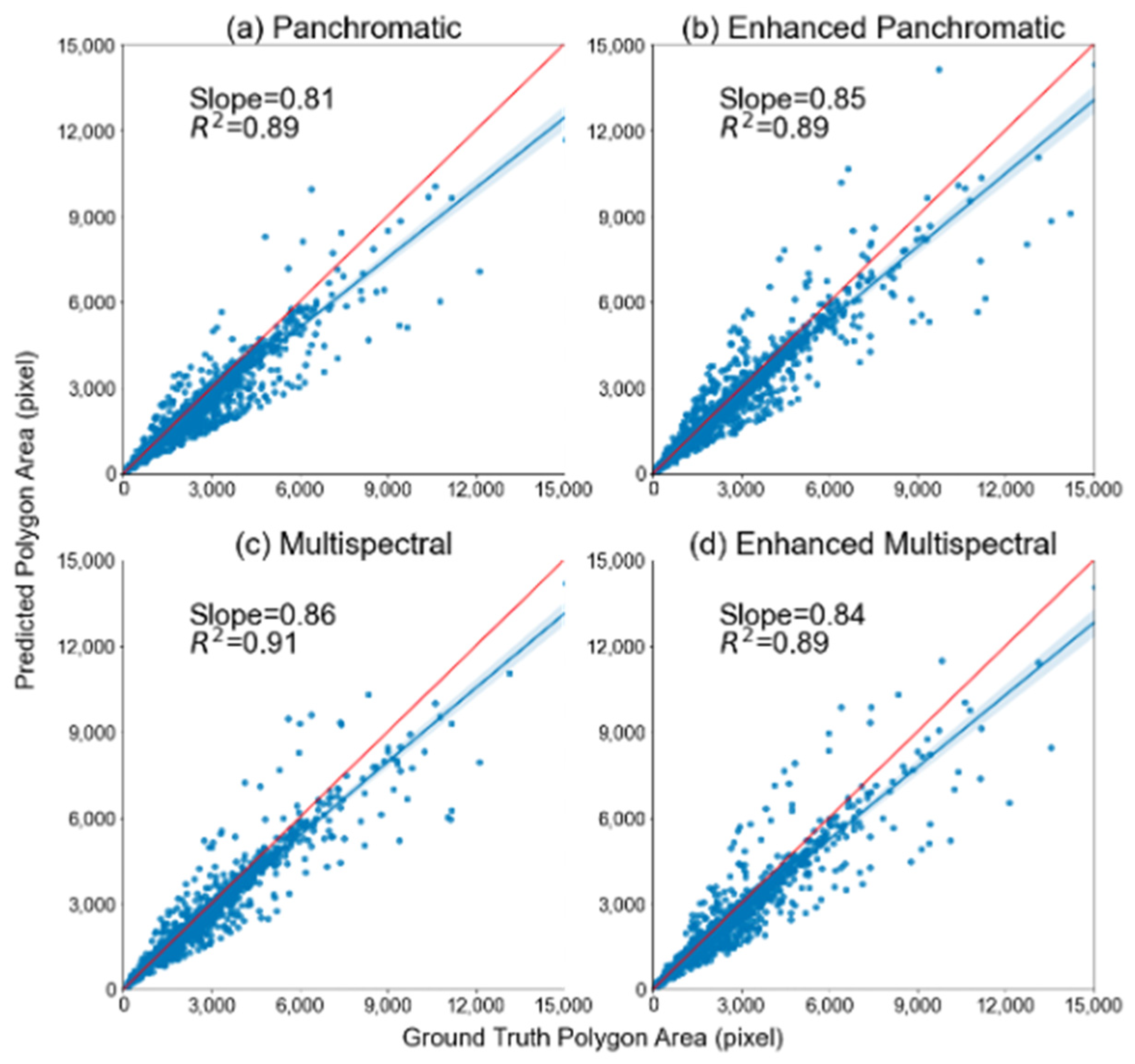
To compare the efficacy in the detection and delineation of several different imagery types in mapping smallholder field boundaries, including panchromatic, pan-sharpened multi-spectral, and edge-enhanced imagery (all with a spatial resolution of 0.5 m).
(2)
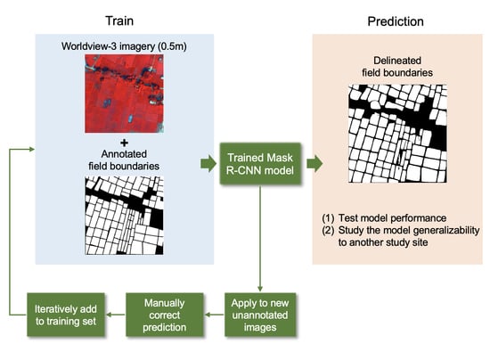
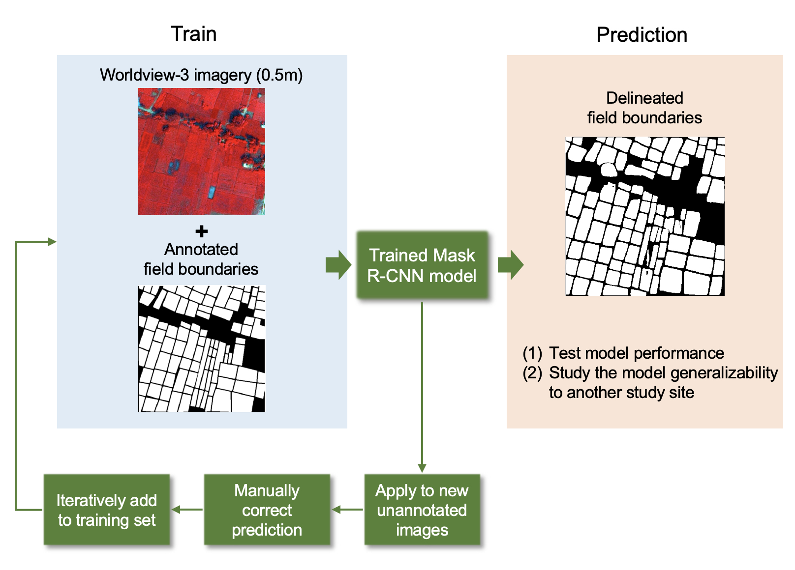
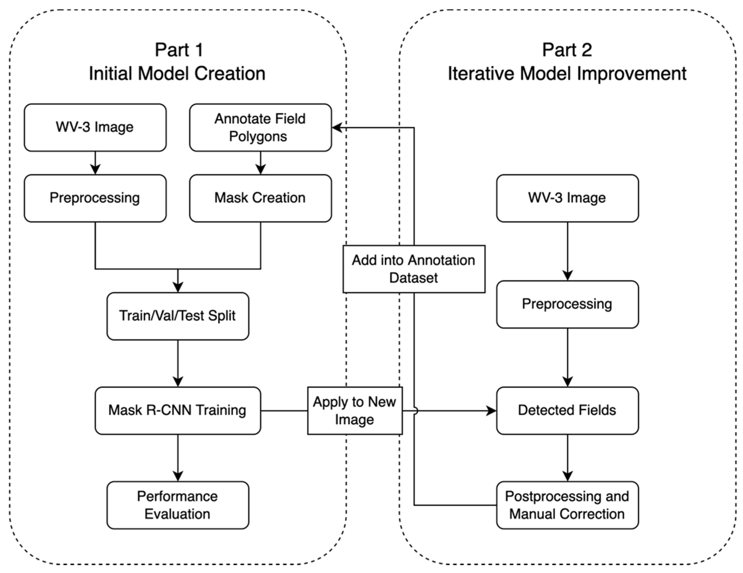
To develop an iterative approach to efficiently collect training data, which relied on annotating incorrectly predicted field boundaries from an initial Mask-RCNN model, and assessing how much our model accuracy improved relative to the amount of additional work needed to add additional training data using our iterative approach.
(3)
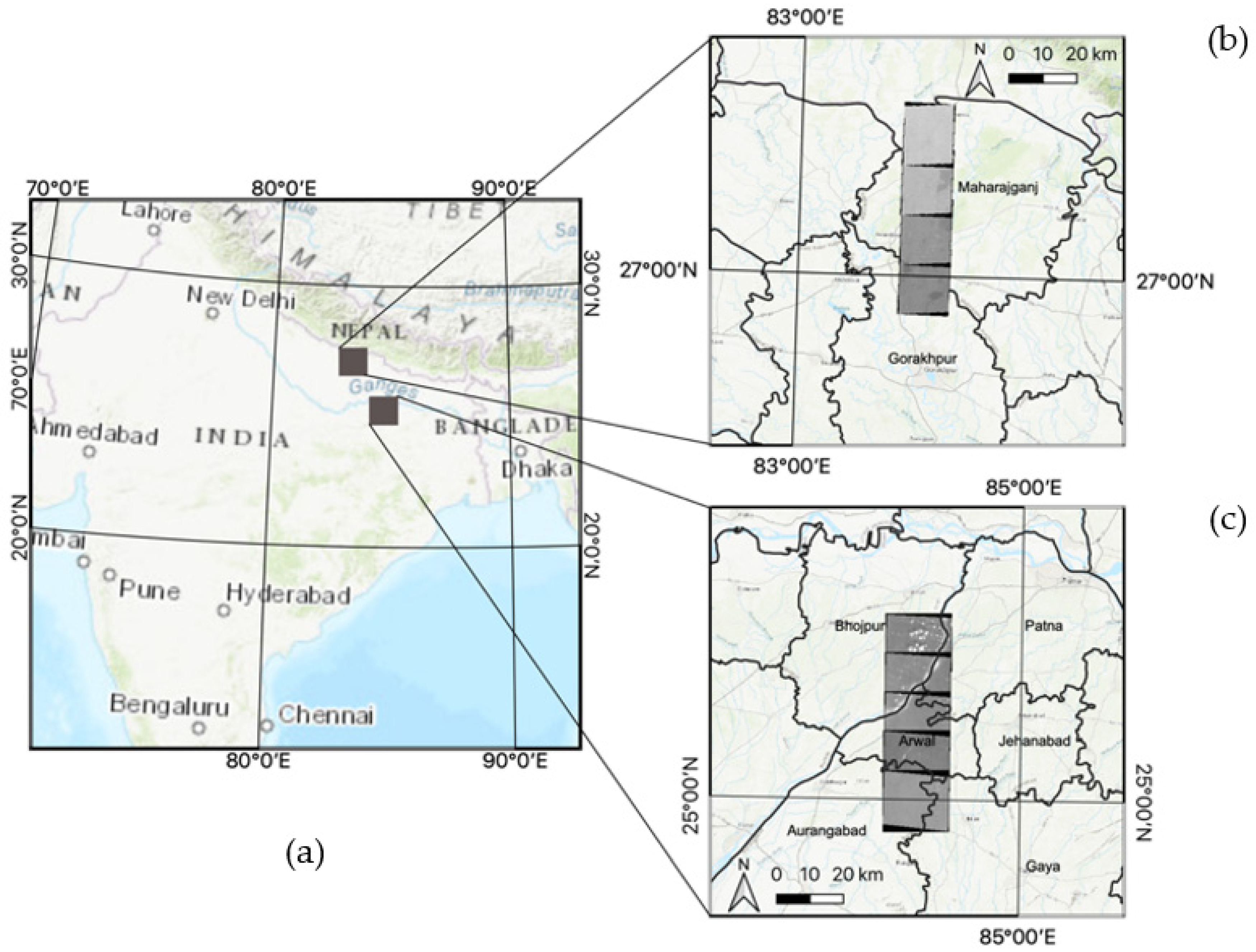
To test the generalizability of our model by applying a model that we trained in Bihar, India, to a site in Uttar Pradesh, India, a neighboring state where we did not use any data for calibrating our model.

2. Study Area

We conducted our study in Northeast India, in the states of Bihar and Uttar Pradesh in the eastern Indo-Gangetic Plains (IGP). This region is highly agrarian, with over 80% of the population in Bihar and over 60% of the population in Uttar Pradesh employed in agriculture [31,32]. Agriculture covers over 80% and 68% of the land area in Bihar and Uttar Pradesh, respectively. Both states are dominated by smallholder farms, with an average farm size in Bihar of 0.39 ha and an average farm size in eastern Uttar Pradesh of 0.64 ha. There are two main growing seasons in this region, the monsoon season (kharif) and the winter (rabi) season. The monsoon growing season starts in June and lasts until October, and most farmers plant rice during this season. The winter season spans from November to April, with most farmers planting wheat during this season [12,33]. The main region for training/validating/testing our method was a 20 by 65 km2 region in Bihar where five WV-3 scenes were available (Figure 1c). The secondary study area for assessing the generalizability of our model was a 15 by 63 km2 region in eastern Uttar Pradesh, where four WV-3 scenes were available (Figure 1b).

3. Methods

3.1. General Workflow

We conducted two broad steps, termed Part 1 and Part 2 (Figure 2), to use Mask R-CNN to delineate smallholder field boundaries using WV-3 imagery. In Part 1 (Figure 2), we (1) acquired and preprocessed the WV-3 satellite imagery; (2) created masks of field boundary annotation based on WV-3; (3) implemented segmentation; and (4) conducted performance evaluations. In Part 2 (Figure 2), we (1) ran the trained model based on unannotated images; (2) identified incorrectly delineated field polygons from Part 1; and (3) manually corrected field boundaries using visual interpretation of imagery. We then included these corrected field boundary data as additional training data in subsequent model predictions. We refer to the annotated dataset from Part 1 as ‘the original dataset’, the iteratively annotated dataset from Part 2 as ‘the iterative dataset’, and data from both Parts 1 and 2 as the ‘final dataset’. To study the generalizability of our field boundary delineation model, we applied the Mask R-CNN models that we trained in Bihar to the second study site, Uttar Pradesh, where we used no data for model calibration.

3.2. Satellite Image Acquisition and Preprocessing

For Bihar, a total of five WV-3 (Maxar Technologies, Inc., Westminster, CO, USA) low-cloud (<5%) satellite image tiles were acquired for 29 October 2017. We acquired both panchromatic imagery (465–800 nm, 0.5 m spatial resolution) and multispectral imagery (2 m spatial resolution) for the same extent. The images were Level 2A radiometrically corrected images and we did not perform further atmospheric correction. For Uttar Pradesh, four WV-3 satellite image tiles were acquired for 23 February 2018. The scenes were cloud-free, radiometrically corrected, and sensor-corrected Level 1B products. Given that these were Level 1B products, several additional preprocessing steps were conducted prior to use in our Mask R-CNN model. To geometrically correct and geolocate the image scenes, we used vendor-provided image support data (ISD), including spacecraft telemetry (attitude and ephemeris data) and geometric calibration files in ArcGIS Pro 2.7 (ESRI, Redlands, CA, USA). To normalize for topographic relief and to improve geolocation accuracy, the CGIAR Shuttle Radar Topography Mission (SRTM) 90 m digital elevation model (DEM) was applied as a coarse DEM for each scene, which contained a rational polynomial coefficient (RPC) sensor model [34,35,36]. The geometrically corrected images were then projected to WGS-84 UTM Zone 44N with cubic convolution at a 0.5 m resolution for panchromatic imagery, and at a 2.0 m resolution for multispectral imagery.
The near infrared 1 (770–895 nm), red (630–690 nm), and green bands (510–580 nm) were pan-sharpened to a 0.5 m spatial resolution with the panchromatic band using the gdal_pansharpen.py function from the GDAL library [37] with bilinear resampling to create a false color composite image. Given that each WV-3 tile was large (more than 36,000 by 33,000 pixels) and computationally intensive to process, we cropped our WV-3 tiles into smaller tiles that were 1024 by 1024 pixels in size. To obtain field boundary data to train, validate, and test our Mask R-CNN models, we randomly selected 45 tiles from the Bihar site and 9 tiles from the Uttar Pradesh site and annotated field polygons based on visual interpretation of the imagery (Section 3.3). We then scaled each image tile to 0–255 (8 bits) using the 0.2 and 0.98 percentile values to improve the visual clarity of the image. Finally, to assess whether edge enhancement and noise removal improved field boundary detection accuracy, we applied edge enhancement to both the panchromatic and pan-sharpened multispectral data. Specifically, we applied the unsharp masking algorithm [38] by following Equation (1) as follows:
Edge   Enhanced   Image   =   Original   Image   + ( Original   Image     Blurred   Image )   ×   Weighting   Factor .
In the equation, the term ( Original   Image     Blurred   Image ) ×   Weighting   Factor refers to the sharpening component. By multiplying a weighting factor larger than 1, the equation can increase the high-frequency components (e.g., edges) in the images, while reducing the noise level. We used a Gaussian standard deviation of 10 for the Gaussian filter and a weighting factor of 2 for Equation (1) based on the visual results. All the image preprocessing steps were implemented using the OpenCV [39], GDAL [37], and Pillow libraries [40] in Python.

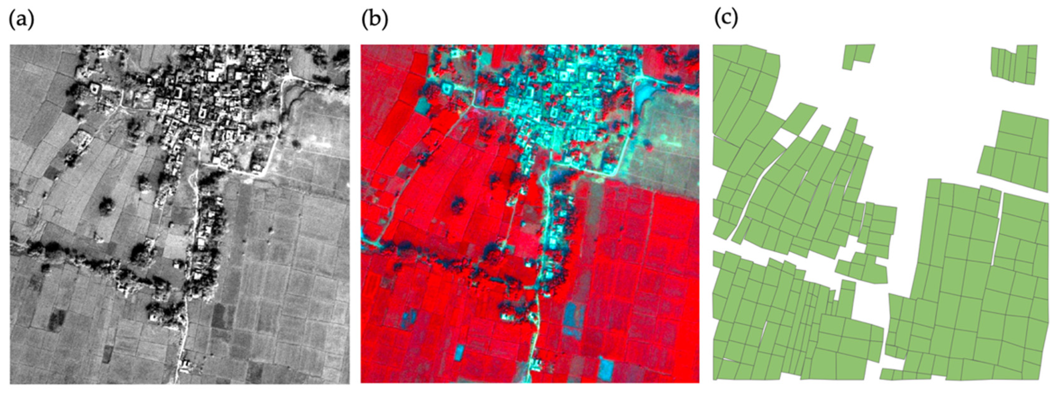
3.3. Field Boundary Annotation and Mask Creation

We manually digitized field boundaries as vector polygons using visual interpretation of both the panchromatic and the color composite imagery using QGIS software [41] (Figure 3). Some boundaries were difficult to identify using only one type of imagery. For example, previous studies have shown that panchromatic images are better for identifying textural transitions related with field boundaries, and multispectral images are better for distinguishing different crop types [21]. Therefore, we examined both WV-3 panchromatic and WV-3 multispectral imagery when annotating field boundaries, and in the cases where field boundaries were ambiguous in both datasets, we examined high-resolution satellite imagery from base maps (Maxar Technologies, Inc., Westminster, CO, USA) in the Google Earth Engine (GEE) [42]. Although we acknowledge that the acquisition date of the imagery in GEE is different than that of our WV-3 imagery, based on local knowledge of the area, we believe that field boundaries did not change drastically from year to year or season to season. To limit potential errors caused by the use of GEE data, we constrained its use to fewer than 5% of all polygons and only in situations where boundaries in the WV-3 imagery were extremely unclear.
We digitized 12,298 polygons across 45 cropped tiles in Bihar and 2266 polygons across 9 cropped tiles in Uttar Pradesh, using a set of consistent rules (Table S1 and Figure S1). Since instance segmentation models require ground truth masks where each field polygon represents a unique separated object, we rasterized the shapefile into a ground truth mask. Because we used the snapping tool during the digitization process to minimize gaps and overlap errors, rasterization resulted in stitched field polygons. To represent the real-world boundary width and ensure that adjacent field polygons remained separated, we then applied a buffer of −1 m to all polygons. All analyses were conducted using the GDAL [37] and scikit-image [43] libraries in Python.

3.4. Instance Segmentation and Model Implementation

Mask R-CNN is one of the state-of-art frameworks for instance segmentation with high simplicity and effectiveness. It combines semantic segmentation and object detection tasks together by generating bounding boxes and a segmentation mask. It is an intuitive extension of the Faster R-CNN method and has two stages. At a high level, Mask R-CNN consists of several modules: (1) a backbone structure that serves as a feature extractor and a feature pyramid network to better present features at different scales; (2) a region proposal network for generating a region of interest (RoI); (3) an RoI classifier for class prediction of each RoI and a bounding box regressor for refining the RoI; and (4) an FCN with RoIAlign and bilinear interpolation for predicting a pixel-accurate mask [24]. The total loss of the training process is a multi-task loss, calculated by adding mask loss, class loss, and box regression loss.
We used the Mask R-CNN implementation from GitHub (https://github.com/matterport/Mask_RCNN, accessed on 1 June 2020) [44], which is built on Keras [45] and TensorFlow [46], for object detection and segmentation. Following a transfer learning paradigm, we fine-tuned the pre-trained weights of the ResNet 101 model, which reduces the model training time. Specifically, this model had been previously trained using the Microsoft Common Objects in Context (COCO) dataset, which enabled the ResNet to start with good models of many features, including but not limited to low-level ones (e.g., edges, corners, and gradients), to segment fields as a new object class. Due to the slow computational speed when running the models on 1024 × 1024 pixel tiles, we further cropped our 45 annotated tiles (1024 × 1024 pixels) into 180 tiles (512 × 512 pixels). To avoid overfitting, a common challenge in image segmentation using deep learning methods, we split the original 180 annotated tiles into training/validation/testing datasets using the ratio 80%/10%/10%. The validation dataset was used to identify the most generalizable Mask-RCNN model based on the validation loss curves. We chose the model weights where the validation loss reached its lowest value to minimize the chance of overfitting our data (Figure S3). To introduce variety into our training data, we applied data augmentation, a useful technique to artificially generate image samples through a series of image transformations to existing images [47]. We randomly selected zero to two types of the following operations: horizontal flips, vertical flips, 90°/180°/270° rotation, 80–150% brightness changes, and Gaussian blurs. Geometric transformations such as flips were applied identically to both the input and label images. We only applied this data augmentation to the training dataset to ensure that we minimized the chance of overfitting our data. Our training model was trained using stochastic gradient descent with a batch size of two images. The learning rate was set to 0.001 based on previous studies that applied Mask R-CNN to high-resolution remote sensing imagery to map features [48,49,50]. A learning momentum of 0.9 and a weight decay of 0.0001 were used, similarly to the original Mask R-CNN paper [24]. We built our Mask R-CNN model on the backbone of ResNet-101 and trained the ResNet-101 Stage 3 and up for 100 epochs, ResNet 101 Stage 4 and up for 60 epochs, and ResNet 101 layers for 40 epochs. Each epoch took approximately 350 s to finish. All experiments were conducted on Amazon Web Services (AWS) and utilized a p2.xlarge instance, for which we used an NVIDIA Tesla K80 GPU and 61 GB RAM.

3.5. Performance Evaluation

We evaluated model performance considering both detection accuracy and delineation accuracy. Detection accuracy verified how well our model could correctly detect a smallholder field, whereas delineation accuracy verified how well our model determined which pixels were included in the field. The detection accuracy was evaluated based on the bounding boxes and the delineation accuracy was evaluated based on the masks. We assessed the precision, recall, the F1 Score, and the average precision (AP) metrics (Table S2) of the bounding boxes and masks detected in Mask R-CNN for detection and delineation accuracy, respectively. We defined a correctly detected or delineated field based on the intersection over union (IoU) (Figure S2) threshold of 0.50. A correctly detected or delineated field, or true positive (TP), occurred when an IoU value greater than 0.5 was achieved considering the amount of overlap between the predicted and ground truth field. In contrast, a false positive (FP) occurred when a detected or delineated field had an IoU value less than 0.5 between the predicted and ground truth field or when duplicate detections or delineation existed. A false negative (FN) occurred when the ground truth field had an IoU value less than 0.5 when compared to a detected or delineated field. Although an IoU of 0.75 is typically also used in natural image instance segmentation studies [24], we found that this threshold was too high for our task, similarly to other studies that have attempted to map objects using noisy satellite image data [50,51].
In addition to the above metrics, we assessed the mean IoU of all correctly delineated fields (TP), which was calculated by comparing each correctly delineated field mask with the corresponding ground truth mask [50]. We also reported the mean area of all correctly delineated field masks with the corresponding field masks (in both square meters and the number of pixels) and the mean area of all delineated field masks with the mean area of all ground truth field masks (in both square meters and the number of pixels). In this way, we could measure if our model overestimated or underestimated the field polygon area.

3.6. Postprocessing and Iterative Data Collection

We used results from our trained model (Section 3.4) to detect and delineate field polygons. We then visually inspected the predicted fields and (1) manually corrected incorrectly annotated fields and (2) manually digitized missing field boundaries using visual interpretation of the WV-3 panchromatic, WV-3 multispectral, or GEE imagery as detailed in Section 3.3. Before manually adjusting field boundaries, we (1) added geographical location information, (2) applied convex hull smoothing to reduce boundary irregularities, and (3) merged four neighboring 512 × 512 pixel tiles into one 1024 × 1024 pixel tile to ensure a consistent spatial extent, as was used in the training data annotation steps (Section 3.3). We performed this iterative polygon delineation method on 160 tiles, which resulted in 11,278 additional polygons. We did not apply a −1 m buffer to this iterative dataset since our model inherently delineated fields with this buffer. We added this iterative dataset (n = 11,278 polygons) to the original dataset (n = 12,298 polygons) to produce a final dataset of 23,576 polygons. We split all annotated tiles in the final dataset into training/validation/testing datasets using the ratio 80%/10%/10% as we performed in Section 3.4, resulting in 18,920, 2276, and 2380 polygons in the training/validation/testing datasets, respectively (Table 1). We then reran the instance segmentation and conducted accuracy assessments using this final dataset for training, testing, and validation.

3.7. Applying Mask R-CNN Model to Second Test Site

To assess the model’s generalizability, we applied the model trained in Bihar to our second test site in Uttar Pradesh, where no calibration data were used to train the model. We used the model weights trained using the ‘final dataset’ from the Bihar site for each respective image type; for example, we applied the model trained using the panchromatic image in Bihar to the panchromatic image in Uttar Pradesh. The model performances were evaluated using 2266 polygons across 36 WV-3 tiles that were 512 × 512 pixels in size (Section 3.2), as described in Table 2. We ensured that the number of test polygons used in Uttar Pradesh (n = 2266) was similar to the number of test polygons used in Bihar (n = 2380 polygons), which ensured consistency when evaluating performance. The same evaluation metrics for detection and delineation were used as in the Bihar site (Section 3.5).

4. Results

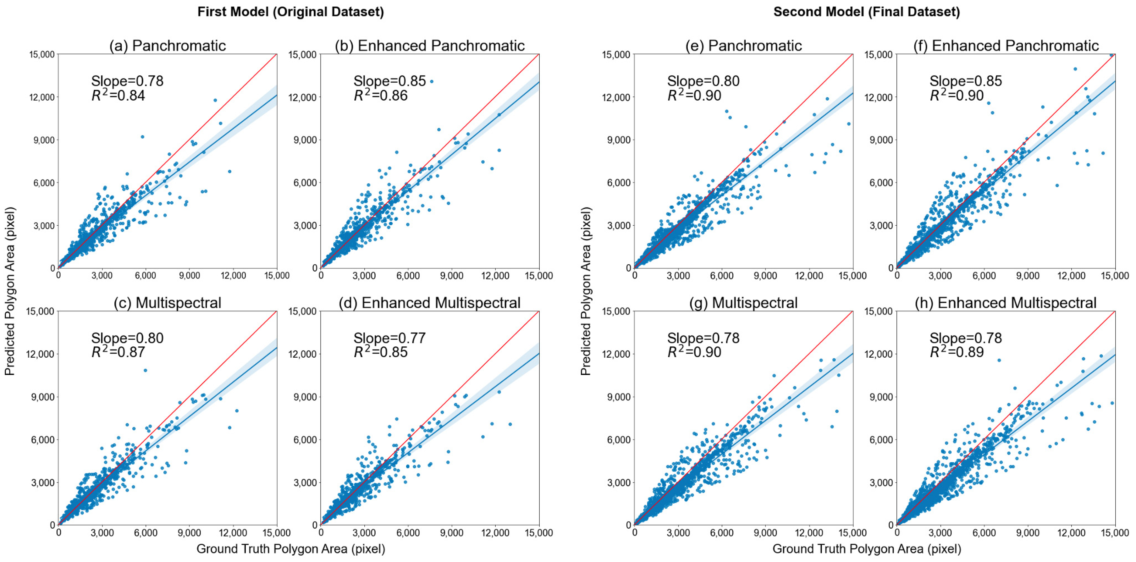
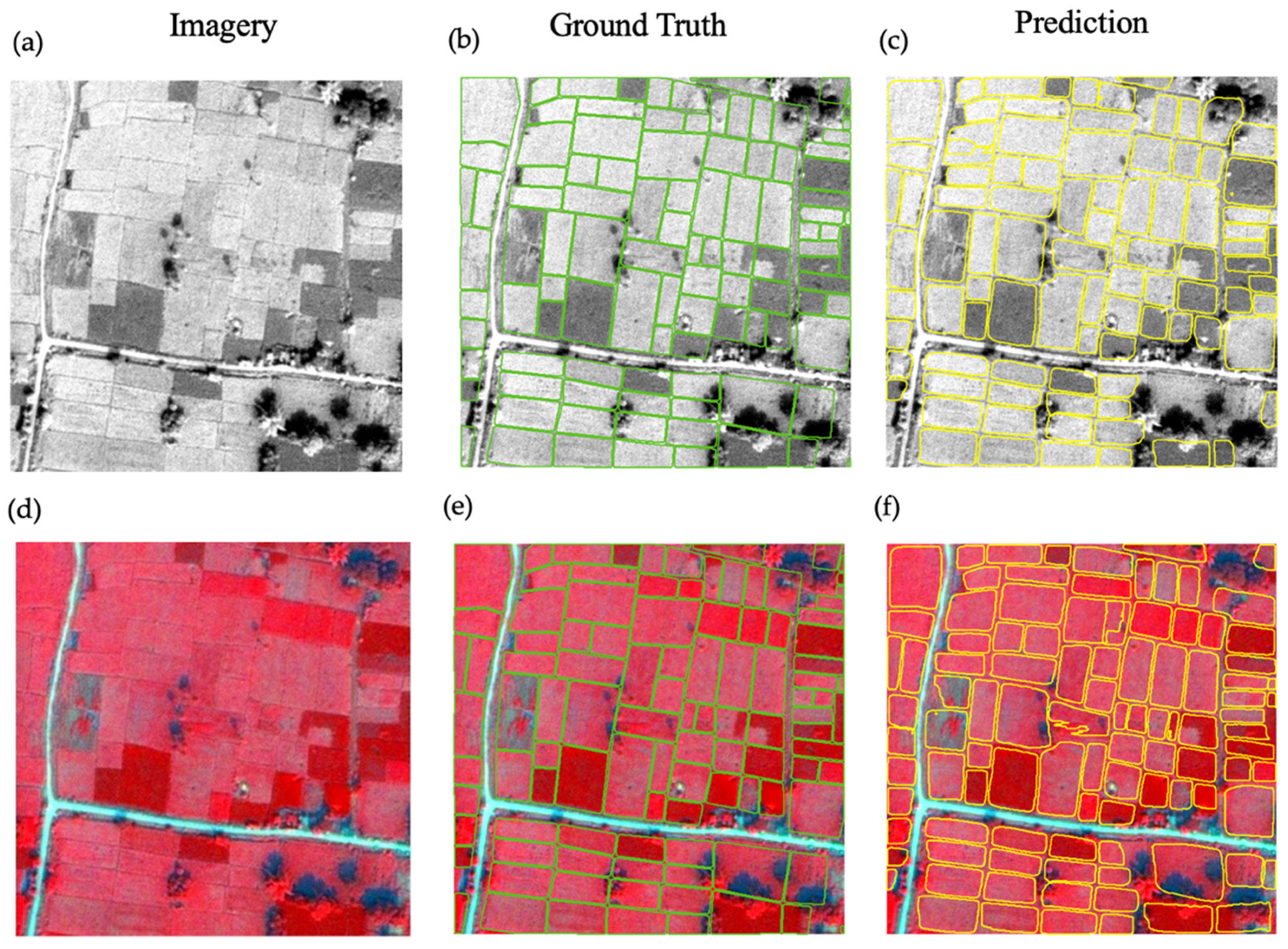
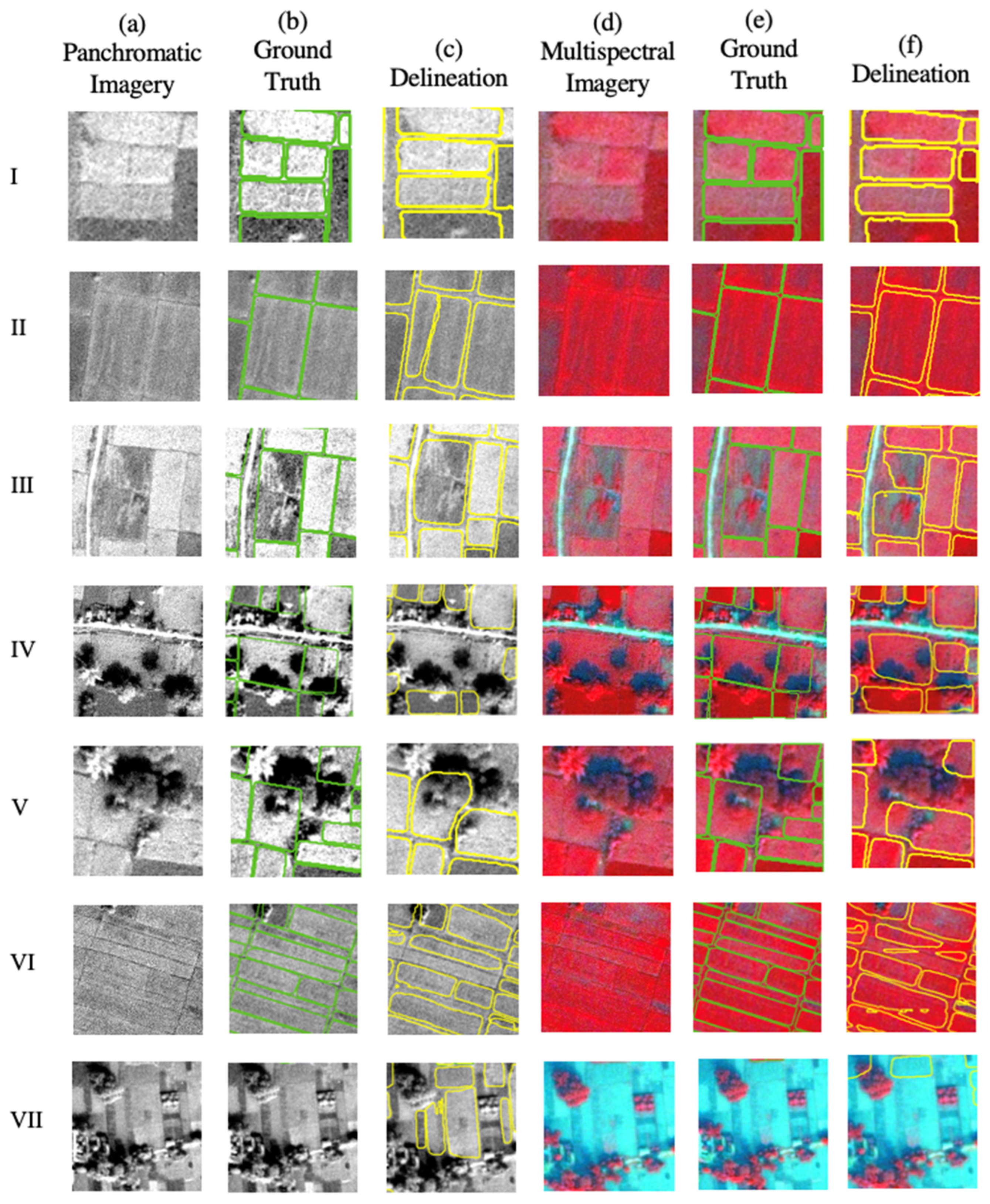
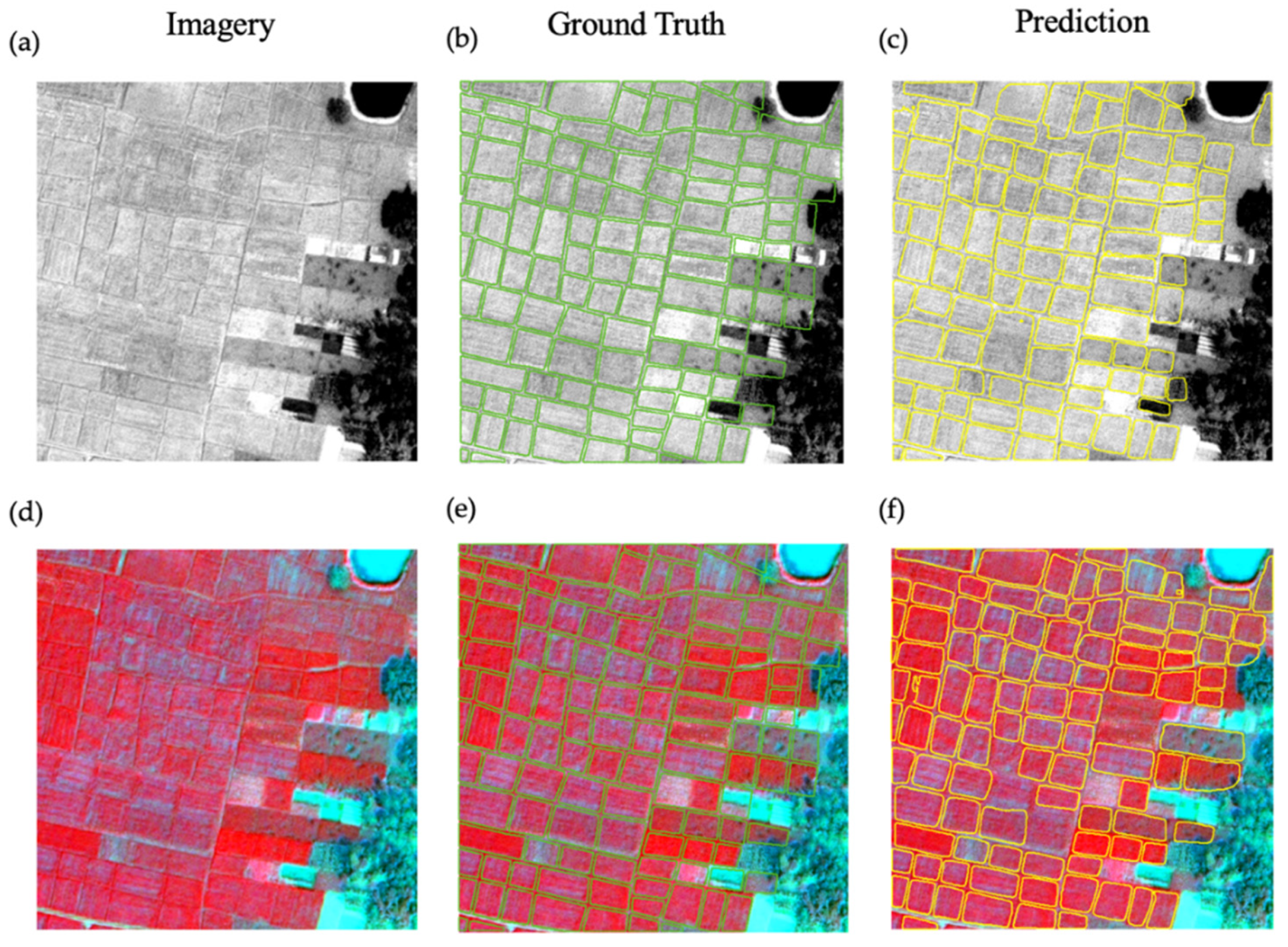
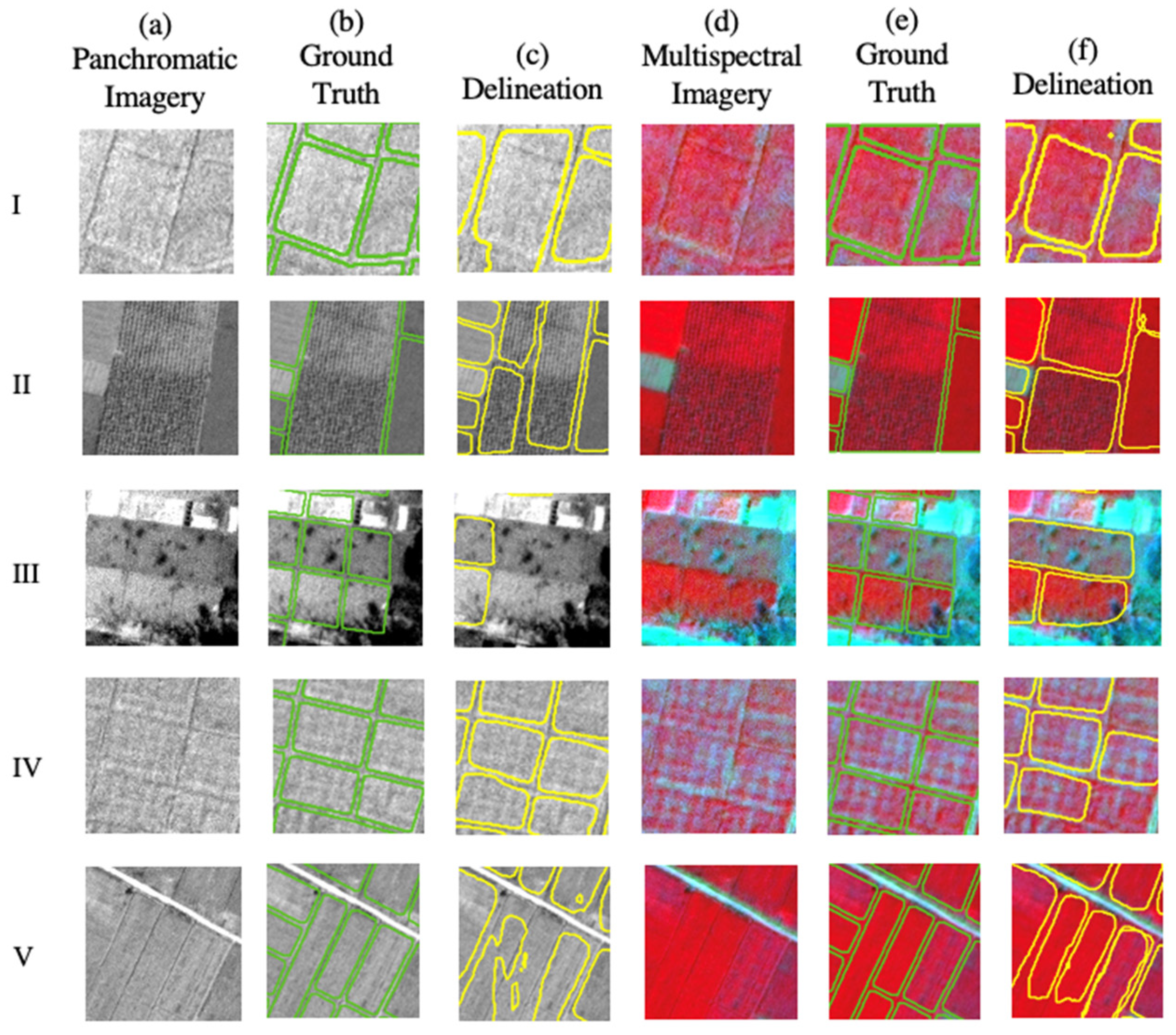
4.1. Accuracy of Using WV-3 in Bihar

Table 3 shows the detection accuracy assessment results for the first model, trained using the original dataset, and the second model, trained using the final dataset (Figure 2). These results were obtained for our site in Bihar where the model was calibrated. Table 3 also shows the difference in detection accuracy for each of the four image types—panchromatic, pan-sharpened multispectral, edge-enhanced panchromatic, and edge-enhanced pan-sharpened multispectral imagery. The F1 Scores and the AP values were similar across the four image types, with the models using edge-enhanced imagery achieving slightly higher accuracies in the second model. With the original dataset, the number of detected fields was smaller than the number of ground truth fields, as indicated by the number of false positives (FP) and false negatives (FN); there were 27–28% false positives and 30–36% false negatives across all models. In contrast, the number of detected fields from the final dataset was larger than the number of ground truth fields; there were 27–30% false positives and 22–25% false negatives across all models. The second model, which included the iteratively trained dataset, outperformed the first model across all image types in terms of the F1 scores and AP values.
Table 4 shows the delineation accuracy assessment results for the first model, trained using the original dataset, and the second model, trained using the final dataset. We also present the results for each of the four image types. The F1 Scores and AP values were similar for all four types of data, with the model that used enhanced multispectral imagery performing slightly better than the models that used other image types. In addition, the second model, which included the iteratively trained dataset, outperformed the first model, based on the F1 Scores and AP values. Similarly to the detection accuracy results, the number of delineated fields from the original dataset was smaller than the number of fields from the ground truth dataset, and the number of delineated fields from the final dataset was larger than the number of fields from the ground truth dataset.
Table 5 shows the mean IoU values, the mean ground truth area, and the mean delineated area for all of the correctly delineated fields. Table S3 shows the mean area of all ground truth field masks and the mean area of all delineated field masks. Across all models, the delineated mask areas were smaller than the ground truth areas (Table 5 and Table S3). Unsurprisingly, plots comparing ground truth and correctly delineated field polygons indicated improved delineation when additional training data were used. The initial models resulted in mean IoU values of 0.80, slopes that ranged from 0.77 to 0.85, and R-squared values that ranged from 0.84 to 0.87 (Figure 4) for all of the four image types. In comparison, the model trained using the final dataset performed better, with IoU values ranging from 0.83 to 0.84, slopes ranging from 0.78 to 0.85, and R-squared values ranging from 0.89 to 0.90 (Figure 4). Among the four types of imagery used, the model using enhanced panchromatic imagery showed the best performance.
Overall, there were several common delineation issues in our results (Figure 5, Figure 6 and Figures S4 and S5). A common delineation error of under-segmentation occurred when several fields were classified as one field due to obscured or marginally visible boundaries (Figure 6I and Figure S5I). There were also cases of over-segmentation, where one field was detected and delineated as two or more fields (Figure 6II, columns b and c). In cases of high within-field crop variation, the model mistakenly identified this variation as a boundary edge when using multispectral imagery (Figure 6III, columns e and f), whereas the models using the other three imagery types were better able to delineate the field boundaries (Figure 6III and Figure S5III). Occlusion also influenced results. For example, trees at field edges often caused boundary delineation issues (Figure 6IV and Figure S5IV). In addition, the model sometimes could not detect fields accurately at the edge of image tiles (Figure 6V and Figure S5V; upper and right edges are the image edges). Finally, all models failed to detect narrow and long fields when the image tiles consisted primarily of such fields (Figure 6VI and Figure S5VI) and produced false positives in unplanted fields, where it was difficult to visually observe boundaries (Figure 6VII and Figure S5VII).

4.2. Generalizability of Models in Uttar Pradesh

To test the generalizability of the Mask R-CNN models built using WV-3 imagery in Bihar, we used the second model weights from Section 4.1 to detect and delineate field polygons in a new site in Uttar Pradesh. We used no data from Uttar Pradesh to calibrate our models, and thus the performance evaluation in this site represents how well our models may be generalized to other smallholder sites.
Table 6 shows the detection accuracy results. Multispectral imagery obtained the highest accuracy across all image types, with an F1 score of 0.78 and an AP of 0.69. We found that the F1 score and AP values of the models applied in Uttar Pradesh reached similar accuracies as when applied in Bihar (Table 3), where the model was trained. There were some small differences in terms of which image type performed best; in Bihar, the enhanced multispectral imagery performed the best, whereas in Uttar Pradesh, the multispectral imagery performed the best. Furthermore, precision was generally higher in Uttar Pradesh compared to Bihar, whereas the recall was generally lower in Uttar Pradesh compared to Bihar.
Table 7 shows the delineation accuracy results of the models applied in Uttar Pradesh. The F1 scores and the AP values were similar across the four different image types, with multispectral imagery achieving slightly higher accuracy than the other image types. We found that the F1 scores and AP values of the models applied in Uttar Pradesh were similar to those of the models applied in Bihar. The main difference was that the model that used the enhanced multispectral image performed the best in Bihar, whereas the model that used multispectral imagery performed the best in Uttar Pradesh.
Table 8 shows the mean IoU values, the mean ground truth area, and the mean delineated area measured in pixels for all the correctly delineated fields in Uttar Pradesh. Table S4 shows the mean area of all ground truth field masks and the mean area of all delineated field masks in Uttar Pradesh. Across all models, we found that the delineated polygon areas were smaller than the ground truth areas, except when using the enhanced panchromatic imagery and considering all delineated fields (Table S4). The models resulted in mean IoU values that ranged from 0.83 to 0.85 (Table 8), slopes that ranged from 0.81 to 0.86, and R-squared values that ranged from 0.89 to 0.91 (Figure 7) for all four image types. These values were generally higher than the values obtained from models in Bihar (Table 5 and Table 8).
Overall, there were several common delineation issues in the models applied to the site in Uttar Pradesh (Figure 8, Figure 9 and Figures S6 and S7). The first common delineation error was under-segmentation (Figure 9I and Figure S7I, columns b and c; Figure 9III, columns e and f). There were also cases of over-segmentation (Figure 9II and Figure S7II, columns b and c) in cases where there was high within-field crop variation. When the field boundaries were not distinct and within-field variations were comparatively high, the models always failed to detect any polygons (Figure 9III,IV, Figure S7III,IV) or generated irregular boundaries (Figure 9V and Figure S7V). Unlike our models in Bihar, we did not encounter problems with long or unplanted fields as they were not prevalent in the image tiles that we used for testing in Uttar Pradesh.

5. Discussion

Our work demonstrates the potential of Mask R-CNN to map smallholder field polygons, even in systems with very small fields. We found that our models using WV-3 imagery performed very well, with F1 Scores > 0.72 and AP values > 0.66 for detection and delineation. In general, our models correctly delineated within-field pixels (Table 3 and Table 4, Figure 5 and Figure S4), but underestimated field polygon size (Figure 4, Table 5 and Table S3). This was largely due to imprecise boundary predictions (Figure 6 and Figure S5), which may be caused by fully convolutional networks that ignore object boundaries that are difficult to classify [52]. We found that the model generalized well, with similar accuracies achieved for the test site where no data were used for model training. This suggests that Mask R-CNN may be effective in mapping smallholder field boundaries at scale, even in regions with limited or no training data.
Although our overall accuracies were moderate, there were several consistent issues that led to reduced prediction accuracies across our models. Specifically, Mask R-CNN was challenged when there were indistinct field boundaries visible in the image, boundaries were occluded by trees or shadows, fields had high within-field crop variation, or fields were irregularly shaped (Figure 6, Figure 9 and Figures S5 and S7). Considering each of these points, it is not surprising that the model performed poorly when boundaries were indistinct, as field boundaries were not clearly visible even to the human eye. Trees and shadows led to color variation in the imagery, and this variation resulted in either failure to detect fields or the delineation of curved boundaries. The convex hull approach we used during postprocessing was able to reduce some of these errors by generating smoother closed boundaries. Mask R-CNN also led to over-segmented fields or incorrectly curved boundaries when fields had very high within-field variation, though the presence of such fields was rare. Considering irregularly-shaped, long and narrow fields, we believe Mask R-CNN performed poorly because the boundaries for these fields were often indistinct. These fields were also relatively rare in the landscape, limiting their presence in the training data. These four issues were not very prevalent across the landscape, leading to moderate delineation and detection accuracies despite these consistent issues.
Considering image input type, our results indicate that our models performed similarly well regardless of which image type was used, though there was a small advantage when using multispectral and enhanced multispectral images (an improvement of 1–4% in AP). Though overall accuracies were similar, our visual interpretation of predicted field boundaries suggests that each image type resulted in models with different types of mis-delineations (Figure 6, Figure 9 and Figures S5 and S7). For example, the model using panchromatic imagery was more likely to over-segment fields compared to models that were developed using other image types (Figure 6). In addition, the model using multispectral imagery was better able to delineate fields with boundaries occluded by trees compared to models using other image types (Figure 6IV). Given that each input image type was associated with different types of mis-delineations, it is possible that an ensemble approach that considers the results from multiple models that use each image type may lead to improved overall delineation accuracy [53].
We found that our Mask R-CNN models were generalizable, given that the models trained in Bihar showed similar performance when applied to Uttar Pradesh, where no data were used for model training (Table 3, Table 4, Table 6 and Table 7). Interestingly, the similarity in the results obtained from Bihar and Uttar Pradesh suggests that the image date had little influence on our results. This is because the acquisition date for images from Bihar was at the end of the monsoon growing season when crops were being harvested, and the acquisition date for images from Uttar Pradesh was in the middle of the winter growing season, when crops were reaching peak biomass, and from a different year. Although our results suggest that our model is generalizable to systems other than where it was trained, it is important to note that our sites in Bihar and Uttar Pradesh are similar in several ways; they are geographically close (~250 km), with similar crop types (rice-wheat rotations), and have similar field sizes (mostly < 0.3 ha). Future work should assess how generalizable our model is to other more distant areas in India and to other nations with smallholder farms.
We found that our iterative approach for collecting ground truth data led to improved delineation accuracies, while collecting training data more efficiently. Considering the time needed to collect ground truth data, the iterative approach took half the amount of time to annotate one 1024 × 1024 pixel tile compared to the original annotation method. Interestingly, model improvements were not large (an improvement of 0.04 in mean IoU, 0.04–0.05 in F1 Score, and 0.08–0.09 in AP for detection and delineation for the best performing models), even though we doubled the number of training data by adding 9256 polygons. Based on our results, it is unclear whether the improved accuracy when using the iteratively collected data was due to simply having a larger training sample size, or whether it is also because the second set of training data were collected from poorly performing areas. Furthermore, given that the improvement in accuracy using the iteratively collected training data was modest, it is possible that we could have achieved similar model accuracy with reduced effort if we had used a smaller original training dataset and collected a larger iterative sample. Future work should examine the most effective way to use the iterative annotation approach to achieve high model accuracy with reduced effort.
Although our results suggest that Mask R-CNN can successfully map smallholder field boundaries, there are several important avenues for future work. First, though we found that our model was generalizable to another study site where no data were used to train the model, future work should examine how generalizable the model is to more disparate smallholder systems. Our model resulted in higher accuracies than a previous study that used Mask R-CNN to map field boundaries in regions with larger field sizes [25], and this may be because we evaluated our models in a relatively similar region (all sites were part of the rice-wheat cropping system in northeast India). Second, we focused on using only one image date for delineation, but it is possible that including multiple images that account for phenological differences could improve boundary detection performance, as found in previous works [54,55]. Third, future work should assess model accuracy when using field boundary information collected on the ground. Although field boundaries were largely visible when we examined multiple sources of imagery, there were a handful of cases where we were unable to digitize fields accurately due to unclear field boundaries. Finally, though our model performed well using very-high-resolution WV-3 imagery, these data are not readily available, and future work should assess the ability of our algorithm to use other sources of high-resolution imagery that are more readily available, such as PlanetScope imagery.

6. Conclusions

In conclusion, Mask R-CNN applied to very-high-resolution WorldView-3 imagery was able to accurately map smallholder field boundaries, even in regions such as Northeast India where field sizes are very small. Our results suggest that image type does not largely influence the results, though consistent biases in detection and delineation existed with each image type, suggesting that an ensemble approach may lead to higher overall accuracy values. Our results also suggest that Mask R-CNN models are generalizable, given that our models achieved similar accuracies when applied to a new test site where no data were used for model calibration and where imagery were collected during a different season and year. Finally, we developed an iterative approach to collect training data, which may reduce the overall effort required to obtain the data necessary to run such deep learning models.

Supplementary Materials

The following supporting information can be downloaded at: https://www.mdpi.com/article/10.3390/rs14133046/s1, Table S1: Digitization rules; Table S2: Detection and delineation accuracy metrics; Table S3: Mean area of all ground truth field masks and mean area of all delineated field masks in Bihar from models trained using WV-3 in Bihar; Table S4: Mean area of all ground truth field masks and mean area of all delineated field masks in Uttar Pradesh from models trained using WV-3 in Bihar; Figure S1: Example images that highlight several of our annotation rules; Figure S2: Intersection over union of bounding boxes and masks; Figure S3: The training and validation loss curves of the first and the second model for different types of imagery; Figure S4: One example of a 512 × 512 pixels WV-3 enhanced tile in Bihar; Figure S5: Examples of common issues (I to VlI, detailed in text) across different model results (columns a through f) from Bihar; Figure S6: One example of a 512 × 512 pixels WV-3 enhanced tile in Uttar Pradesh; Figure S7: Examples of common issues (I to VlI, detailed in text) across different model results (columns a through f) from Uttar Pradesh.

Author Contributions

Conceptualization, M.J. and W.M.; methodology, W.M., D.F. and M.J.; formal analysis, W.M.; data curation, W.M. and H.W.; writing—original draft preparation, W.M.; with edits from M.J.; writing—review and editing, W.M., H.W., D.F., W.Z., I.H., J.M.G., D.V.B. and M.J. All authors have read and agreed to the published version of the manuscript.

Funding

This research was funded by the NASA Land Cover and Land Use Change Grant NNX17AH97G awarded to M.J.

Data Availability Statement

Data and code used to conduct the study are available from the first author, W.M., upon reasonable request. High-resolution WV-3 imagery used in this study are not available.

Acknowledgments

This research was sponsored by the NASA Land Cover and Land Use Change Grant NNX17AH97G by providing access to high-resolution WV-3 imagery through the NASA Cad-4 database.

Conflicts of Interest

The authors declare no conflict of interest.

References

  1. Haworth, B.T.; Biggs, E.; Duncan, J.; Wales, N.; Boruff, B.; Bruce, E. Geographic Information and Communication Technologies for Supporting Smallholder Agriculture and Climate Resilience. Climate 2018, 6, 97. [Google Scholar] [CrossRef] [Green Version]
  2. Jain, M.; Singh, B.; Srivastava, A.A.K.; Malik, R.K.; McDonald, A.J.; Lobell, D.B. Using Satellite Data to Identify the Causes of and Potential Solutions for Yield Gaps in India’s Wheat Belt. Environ. Res. Lett. 2017, 12, 094011. [Google Scholar] [CrossRef]
  3. Neumann, K.; Verburg, P.H.; Stehfest, E.; Müller, C. The Yield Gap of Global Grain Production: A Spatial Analysis. Agric. Syst. 2010, 103, 316–326. [Google Scholar] [CrossRef]
  4. Wagner, M.P.; Oppelt, N. Extracting Agricultural Fields from Remote Sensing Imagery Using Graph-Based Growing Contours. Remote Sens. 2020, 12, 1205. [Google Scholar] [CrossRef] [Green Version]
  5. Mueller, N.D.; Gerber, J.S.; Johnston, M.; Ray, D.K.; Ramankutty, N.; Foley, J.A. Closing Yield Gaps through Nutrient and Water Management. Nature 2012, 490, 254–257. [Google Scholar] [CrossRef]
  6. Samberg, L.H.; Gerber, J.S.; Ramankutty, N.; Herrero, M.; West, P.C. Subnational Distribution of Average Farm Size and Smallholder Contributions to Global Food Production. Environ. Res. Lett. 2016, 11, 124010. [Google Scholar] [CrossRef]
  7. Sylvester, G. Success Stories on Information and Communication Technologies for Agriculture and Rural Development. RAP Publ. 2015, 2, 108. [Google Scholar]
  8. Garcia-Pedrero, A.; Lillo-Saavedra, M.; Rodriguez-Esparragon, D.; Gonzalo-Martin, C. Deep Learning for Automatic Outlining Agricultural Parcels: Exploiting the Land Parcel Identification System. IEEE Access 2019, 7, 158223–158236. [Google Scholar] [CrossRef]
  9. Marvaniya, S.; Devi, U.; Hazra, J.; Mujumdar, S.; Gupta, N. Small, Sparse, but Substantial: Techniques for Segmenting Small Agricultural Fields Using Sparse Ground Data. Int. J. Remote Sens. 2021, 42, 1512–1534. [Google Scholar] [CrossRef]
  10. Masoud, K.M.; Persello, C.; Tolpekin, V.A. Delineation of Agricultural Field Boundaries from Sentinel-2 Images Using a Novel Super-Resolution Contour Detector Based on Fully Convolutional Networks. Remote Sens. 2020, 12, 59. [Google Scholar] [CrossRef] [Green Version]
  11. Lesiv, M.; Laso Bayas, J.C.; See, L.; Duerauer, M.; Dahlia, D.; Durando, N.; Hazarika, R.; Kumar Sahariah, P.; Vakolyuk, M.; Blyshchyk, V. Estimating the Global Distribution of Field Size Using Crowdsourcing. Glob. Chang. Biol. 2019, 25, 174–186. [Google Scholar] [CrossRef] [PubMed]
  12. Jain, M.; Srivastava, A.K.; Joon, R.K.; McDonald, A.; Royal, K.; Lisaius, M.C.; Lobell, D.B. Mapping Smallholder Wheat Yields and Sowing Dates Using Micro-Satellite Data. Remote Sens. 2016, 8, 860. [Google Scholar] [CrossRef] [Green Version]
  13. Mueller, M.; Segl, K.; Kaufmann, H. Edge-and Region-Based Segmentation Technique for the Extraction of Large, Man-Made Objects in High-Resolution Satellite Imagery. Pattern Recognit. 2004, 37, 1619–1628. [Google Scholar] [CrossRef]
  14. Watkins, B.; van Niekerk, A. A Comparison of Object-Based Image Analysis Approaches for Field Boundary Delineation Using Multi-Temporal Sentinel-2 Imagery. Comput. Electron. Agric. 2019, 158, 294–302. [Google Scholar] [CrossRef]
  15. Canny, J. A Computational Approach to Edge Detection. IEEE Trans. Pattern Anal. Mach. Intell. 1986, PAMI-8, 679–698. [Google Scholar] [CrossRef]
  16. Martin, D.R.; Fowlkes, C.C.; Malik, J. Learning to Detect Natural Image Boundaries Using Local Brightness, Color, and Texture Cues. IEEE Trans. Pattern Anal. Mach. Intell. 2004, 26, 530–549. [Google Scholar] [CrossRef]
  17. Alemu, M.M. Automated Farm Field Delineation and Crop Row Detection from Satellite Images. Master’s Thesis, University of Twente, Enschede, The Netherlands, 2016. [Google Scholar]
  18. Belgiu, M.; Csillik, O. Sentinel-2 Cropland Mapping Using Pixel-Based and Object-Based Time-Weighted Dynamic Time Warping Analysis. Remote Sens. Environ. 2018, 204, 509–523. [Google Scholar] [CrossRef]
  19. Chen, B.; Qiu, F.; Wu, B.; Du, H. Image Segmentation Based on Constrained Spectral Variance Difference and Edge Penalty. Remote Sens. 2015, 7, 5980–6004. [Google Scholar] [CrossRef] [Green Version]
  20. Crommelinck, S.; Bennett, R.; Gerke, M.; Yang, M.Y.; Vosselman, G. Contour Detection for UAV-Based Cadastral Mapping. Remote Sens. 2017, 9, 171. [Google Scholar] [CrossRef] [Green Version]
  21. Persello, C.; Tolpekin, V.A.; Bergado, J.R.; de By, R.A. Delineation of Agricultural Fields in Smallholder Farms from Satellite Images Using Fully Convolutional Networks and Combinatorial Grouping. Remote Sens. Environ. 2019, 231, 111253. [Google Scholar] [CrossRef]
  22. Waldner, F.; Diakogiannis, F.I. Deep Learning on Edge: Extracting Field Boundaries from Satellite Images with a Convolutional Neural Network. Remote Sens. Environ. 2020, 245, 111741. [Google Scholar] [CrossRef]
  23. Wang, S.; Waldner, F.; Lobell, D.B. Delineating Smallholder Fields Using Transfer Learning and Weak Supervision. In AGU Fall Meeting 2021; AGU: Washington, DC, USA, 2021. [Google Scholar]
  24. He, K.; Gkioxari, G.; Dollár, P.; Girshick, R. Mask R-CNN. arXiv 2018, arXiv:1703.06870. [Google Scholar]
  25. Quoc, T.T.P.; Linh, T.T.; Minh, T.N.T. Comparing U-Net Convolutional Network with Mask R-CNN in Agricultural Area Segmentation on Satellite Images. In Proceedings of the 2020 7th NAFOSTED Conference on Information and Computer Science (NICS), Ho Chi Minh City, Vietnam, 26–27 November 2020; pp. 124–129. [Google Scholar]
  26. Marshall, M.; Crommelinck, S.; Kohli, D.; Perger, C.; Yang, M.Y.; Ghosh, A.; Fritz, S.; de Bie, K.; Nelson, A. Crowd-Driven and Automated Mapping of Field Boundaries in Highly Fragmented Agricultural Landscapes of Ethiopia with Very High Spatial Resolution Imagery. Remote Sens. 2019, 11, 2082. [Google Scholar] [CrossRef] [Green Version]
  27. Elmes, A.; Alemohammad, H.; Avery, R.; Caylor, K.; Eastman, J.R.; Fishgold, L.; Friedl, M.A.; Jain, M.; Kohli, D.; Laso Bayas, J.C. Accounting for Training Data Error in Machine Learning Applied to Earth Observations. Remote Sens. 2020, 12, 1034. [Google Scholar] [CrossRef] [Green Version]
  28. Tuia, D.; Volpi, M.; Copa, L.; Kanevski, M.; Munoz-Mari, J. A Survey of Active Learning Algorithms for Supervised Remote Sensing Image Classification. IEEE J. Sel. Top. Signal Process. 2011, 5, 606–617. [Google Scholar] [CrossRef]
  29. Lobell, D.B.; Di Tommaso, S.; Burke, M.; Kilic, T. Twice Is Nice: The Benefits of Two Ground Measures for Evaluating the Accuracy of Satellite-Based Sustainability Estimates. Remote Sens. 2021, 13, 3160. [Google Scholar] [CrossRef]
  30. Neigh, C.S.; Carroll, M.L.; Wooten, M.R.; McCarty, J.L.; Powell, B.F.; Husak, G.J.; Enenkel, M.; Hain, C.R. Smallholder Crop Area Mapped with Wall-to-Wall WorldView Sub-Meter Panchromatic Image Texture: A Test Case for Tigray, Ethiopia. Remote Sens. Environ. 2018, 212, 8–20. [Google Scholar] [CrossRef]
  31. Aryal, J.P.; Jat, M.L.; Sapkota, T.B.; Khatri-Chhetri, A.; Kassie, M.; Maharjan, S. Adoption of Multiple Climate-Smart Agricultural Practices in the Gangetic Plains of Bihar, India. Int. J. Clim. Chang. Strateg. Manag. 2018. [Google Scholar] [CrossRef]
  32. Shapiro, B.I.; Singh, J.P.; Mandal, L.N.; Sinha, S.K.; Mishra, S.N.; Kumari, A.; Kumar, S.; Jha, A.K.; Gebru, G.; Negussie, K.; et al. Bihar Livestock Master Plan 2018–19–2022–23; Government of Bihar: Patna, India, 2018.
  33. Government of Uttar Pradesh. Integrated Watershed Management Programme in Uttar Pradesh Perspective and Strategic Plan 2009–2027; Government of Uttar Pradesh: Lucknow, India, 2009.
  34. DigitalGlobe DigitalGlobe Core Imagery Products Guide. Available online: https://www.digitalglobe.com/resources/ (accessed on 20 March 2021).
  35. Jarvis, A.; Reuter, H.I.; Nelson, A.; Guevara, E. Hole-Filled SRTM for the Globe Version 4, Available from the CGIAR-CSI SRTM 90m Database; CGIAR Consortium for Spatial Information: Montpellier, France, 2008. [Google Scholar]
  36. Rahman, M.M.; Robson, A.; Bristow, M. Exploring the Potential of High Resolution WorldView-3 Imagery for Estimating Yield of Mango. Remote Sens. 2018, 10, 1866. [Google Scholar] [CrossRef] [Green Version]
  37. GDAL/OGR Contributors GDAL/OGR Geospatial Data Abstraction Software Library. Available online: https://gdal.org (accessed on 1 June 2020).
  38. Polesel, A.; Ramponi, G.; Mathews, V.J. Image Enhancement via Adaptive Unsharp Masking. IEEE Trans. Image Process. 2000, 9, 505–510. [Google Scholar] [CrossRef] [Green Version]
  39. Bradski, G. The OpenCV Library. Dr Dobbs J. Softw. Tools Prof. Program. 2000, 25, 120–123. [Google Scholar]
  40. van Kemenade, H.; Wiredfool; Murray, A.; Clark, A.; Karpinsky, A.; Gohlke, C.; Dufresne, J.; Nulano; Crowell, B.; Schmidt, D.; et al. Python-Pillow/Pillow 7.1.2 (7.1.2). Available online: https://zenodo.org/record/3766443 (accessed on 1 June 2020).
  41. QGIS organization. QGIS Geographic Information System; QGIS Association: Online, 2021. [Google Scholar]
  42. Gorelick, N.; Hancher, M.; Dixon, M.; Ilyushchenko, S.; Thau, D.; Moore, R. Google Earth Engine: Planetary-Scale Geospatial Analysis for Everyone. Remote Sens. Environ. 2017, 202, 18–27. [Google Scholar] [CrossRef]
  43. Van der Walt, S.; Schönberger, J.L.; Nunez-Iglesias, J.; Boulogne, F.; Warner, J.D.; Yager, N.; Gouillart, E.; Yu, T. Scikit-Image: Image Processing in Python. PeerJ 2014, 2, e453. [Google Scholar] [CrossRef] [PubMed]
  44. Abdulla, W. Mask R-CNN for Object Detection and Instance Segmentation on Keras and TensorFlow. Available online: https://github.com/matterport/Mask_RCNN (accessed on 1 June 2020).
  45. Chollet, F. Keras. Available online: https://keras.io (accessed on 1 June 2020).
  46. Abadi, M.; Agarwal, A.; Barham, P.; Brevdo, E.; Chen, Z.; Citro, C.; Corrado, G.S.; Davis, A.; Dean, J.; Devin, M.; et al. TensorFlow: Large-Scale Machine Learning on Heterogeneous Systems. arXiv 2015, arXiv:1603.04467. [Google Scholar]
  47. Garcia-Garcia, A.; Orts-Escolano, S.; Oprea, S.; Villena-Martinez, V.; Garcia-Rodriguez, J. A Review on Deep Learning Techniques Applied to Semantic Segmentation. arXiv 2017, arXiv:1704.06857. [Google Scholar]
  48. Zhang, W.; Liljedahl, A.K.; Kanevskiy, M.; Epstein, H.E.; Jones, B.M.; Jorgenson, M.T.; Kent, K. Transferability of the Deep Learning Mask R-CNN Model for Automated Mapping of Ice-Wedge Polygons in High-Resolution Satellite and UAV Images. Remote Sens. 2020, 12, 1085. [Google Scholar] [CrossRef] [Green Version]
  49. Bhuiyan, M.A.E.; Witharana, C.; Liljedahl, A.K. Use of Very High Spatial Resolution Commercial Satellite Imagery and Deep Learning to Automatically Map Ice-Wedge Polygons across Tundra Vegetation Types. J. Imaging 2020, 6, 137. [Google Scholar] [CrossRef]
  50. Braga, J.R.G.; Peripato, V.; Dalagnol, R.; Ferreira, M.P.; Tarabalka, Y.; Aragão, L.E.O.C.; de Campos Velho, H.F.; Shiguemori, E.H.; Wagner, F.H. Tree Crown Delineation Algorithm Based on a Convolutional Neural Network. Remote Sens. 2020, 12, 1288. [Google Scholar] [CrossRef] [Green Version]
  51. Li, Y.; Xu, W.; Chen, H.; Jiang, J.; Li, X. A Novel Framework Based on Mask R-CNN and Histogram Thresholding for Scalable Segmentation of New and Old Rural Buildings. Remote Sens. 2021, 13, 1070. [Google Scholar] [CrossRef]
  52. Cheng, T.; Wang, X.; Huang, L.; Liu, W. Boundary-Preserving Mask R-CNN. In Proceedings of the European Conference on Computer Vision, Glasgow, UK, 23–28 August 2020; Springer: Berlin/Heidelberg, Germany, 2020; pp. 660–676. [Google Scholar]
  53. Prathap, G.; Afanasyev, I. Deep Learning Approach for Building Detection in Satellite Multispectral Imagery. In Proceedings of the 2018 International Conference on Intelligent Systems (IS), Funchal, Portugal, 25–27 September 2018; pp. 461–465. [Google Scholar]
  54. Aung, H.L.; Uzkent, B.; Burke, M.; Lobell, D.; Ermon, S. Farm Parcel Delineation Using Spatio-Temporal Convolutional Networks. In Proceedings of the IEEE/CVF Conference on Computer Vision and Pattern Recognition Workshops, Seattle, WA, USA, 14–19 June 2020; pp. 76–77. [Google Scholar]
  55. Debats, S.R.; Luo, D.; Estes, L.D.; Fuchs, T.J.; Caylor, K.K. A Generalized Computer Vision Approach to Mapping Crop Fields in Heterogeneous Agricultural Landscapes. Remote Sens. Environ. 2016, 179, 210–221. [Google Scholar] [CrossRef] [Green Version]
Figure 1. Panel (a) shows our study areas located in Bihar and Uttar Pradesh, India. Panel (b) shows the location of the satellite image scenes across two districts in Uttar Pradesh. Panel (c) shows the location of satellite image scenes across five districts in Bihar. District boundaries are shown in black. Map source: Esri Topo World.
Remotesensing 14 03046 g001
Figure 2. Workflow of building the Mask R-CNN models using WV-3 in Bihar.
Remotesensing 14 03046 g002
Figure 3. (a) Example of panchromatic imagery, (b) multispectral imagery, and (c) digitized field polygons for one 1024 × 1024 pixel tile.
Remotesensing 14 03046 g003
Figure 4. Scatterplots of ground truth mask area (in pixels) on the x-axis versus delineated mask area (in pixels) on the y-axis. Only correctly delineated field masks are included. Plots (ad) represent results for the original model across WV-3 image types in Bihar, and plots (eh) represent results for the final model across WV-3 image types in Bihar. Blue lines with shading represent the linear regression line with 95% confidence intervals, and red lines represent the one-to-one line.
Remotesensing 14 03046 g004
Figure 5. One example of a 512 × 512 pixels WV-3 unenhanced tile in Bihar. Panel (a) shows the original panchromatic image, (b) shows the panchromatic image with ground truth, (c) shows the panchromatic image with delineated field boundaries, (d) shows the original multispectral image, (e) shows the multispectral image with ground truth, and (f) shows the multispectral image with delineated field boundaries. Results are shown for the final model, which included the iteratively collected data. Green lines represent ground truth boundaries and yellow lines represent predicted boundaries.
Remotesensing 14 03046 g005
Figure 6. Examples of common issues (IVII, detailed in text) across different model results (columns (af)) from Bihar. Green lines represent ground truth boundaries, and yellow lines represent predicted boundaries for panchromatic and multispectral imagery, respectively.
Remotesensing 14 03046 g006
Figure 7. Scatterplots of ground truth mask area (in pixels) on the x-axis versus delineated mask area (in pixels) on the y-axis. Only correctly delineated field masks are included. Plots (ad) represent results for each image type for the models applied in Uttar Pradesh. Blue lines with shading represent the linear regression line with 95% confidence intervals, and red lines represent the one-to-one line.
Remotesensing 14 03046 g007
Figure 8. One example of a 512 × 512-pixels WV-3 unenhanced tile in Uttar Pradesh. Panel (a) shows the original panchromatic image, (b) shows the panchromatic image with ground truth, (c) shows the enhanced panchromatic image with delineated field boundaries, (d) shows the original multispectral image, (e) shows the multispectral image with ground truth, and (f) shows the enhanced multispectral image with delineated field boundaries. Results are shown for the final model, which included the iteratively collected data. Green lines represent ground truth field boundaries, and yellow lines represent predicted field boundaries.
Remotesensing 14 03046 g008
Figure 9. Examples of common issues (IV, detailed in text) across the different model results (panels (af)) in Uttar Pradesh. Green lines represent ground truth field boundaries, and yellow lines represent predicted boundaries for panchromatic and multispectral imagery, respectively.
Remotesensing 14 03046 g009
Table 1. Description of training/validation/testing datasets that were used for building and evaluating the models in Bihar.
DatasetThe Number of 512 × 512 Image TilesThe Number of Field PolygonsLocationSource Imagery and Date
Original Dataset of First Test SiteTraining1449664BiharWorldview-3
29 October 2017
Validation181233
Testing181401
Final Dataset of First Test SiteTraining27218,920
Validation342276
Testing342380
Table 2. Description of testing datasets that were used for evaluating the generalizability of models in Uttar Pradesh.
DatasetThe Number of 512 × 512 Image TilesThe Number of Field PolygonsLocationSource Imagery and Date
Dataset of Second Test SiteTesting362266Uttar PradeshWorldview-3 23 February 2018
Table 3. Detection accuracy of mapping smallholder field boundaries in Bihar from models trained using WV-3 data in Bihar. The accuracy metrics from the model with the best F1 score and AP values are highlighted in bold.
TPFPFNPrecisionRecallF1 ScoreAP
First Model (Original Dataset)Panchromatic9863914150.720.700.710.63
Enhanced Panchromatic8973485040.720.640.680.57
Multispectral9533674480.720.680.700.59
Enhanced Multispectral9423544590.730.670.700.60
Second Model (Final Dataset)Panchromatic18619035190.670.780.720.68
Enhanced Panchromatic17966565840.730.750.740.68
Multispectral18297695510.700.770.730.66
Enhanced Multispectral18317235490.720.770.740.68
Table 4. Delineation accuracy of mapping smallholder field boundaries in Bihar from models trained using WV-3 data in Bihar. The accuracy metrics from the model with the best F1 score and AP values are highlighted in bold.
TPFPFNPrecisionRecallF1 ScoreAP
First Model (Original Dataset)Panchromatic9803984210.710.700.700.62
Enhanced Panchromatic9063684950.710.650.680.57
Multispectral9393704620.710.670.690.58
Enhanced Multispectral9333554680.720.670.690.59
Second Model (Final Dataset)Panchromatic18449215360.670.770.720.68
Enhanced Panchromatic17826705980.730.750.740.67
Multispectral18327605480.710.770.740.67
Enhanced Multispectral18277275530.720.770.740.68
Table 5. Mean IoU, mean ground truth area, and mean delineated field area in Bihar from models trained using WV-3 data in Bihar. Only correctly delineated field masks were included to generate this table. The areas are reported in terms of both the number of pixels and square meters (rounded to the nearest integer). The metrics from the model with the best IoU are shown in bold.
Mean IoUMean Ground Truth AreaMean Delineated
Area
(Pixel)(m2)Pixel(m2)
First Model (Original Dataset)Panchromatic0.8023485872220555
Enhanced Panchromatic0.8024156042359590
Multispectral0.8023425862241560
Enhanced Multispectral0.8023205802207552
Second Model (Final Dataset)Panchromatic0.8324576142260565
Enhanced Panchromatic0.8425896472479620
Multispectral0.8326876722368592
Enhanced Multispectral0.8327476872395599
Table 6. Detection accuracy of mapping smallholder field boundaries in Uttar Pradesh with models trained using WV-3 data in Bihar. The accuracy metrics from the model with the best F1 score and AP values are highlighted in bold.
TPFPFNPrecisionRecallF1 ScoreAP
Second Model (Trained with Final WV-3 Dataset in Bihar)Panchromatic19277587390.720.720.720.64
Enhanced Panchromatic18894957770.790.710.750.64
Multispectral20054856610.810.750.780.69
Enhanced Multispectral19645387020.780.740.760.67
Table 7. Delineation accuracy of mapping smallholder field boundaries in Uttar Pradesh with models trained using WV-3 data in Bihar. The accuracy metrics from the model with the best F1 score and AP values are highlighted in bold.
TPFPFNPrecisionRecallF1 ScoreAP
Second Model (Trained with Final Dataset in Bihar)Panchromatic19207657460.720.720.720.64
Enhanced Panchromatic18964887700.800.710.750.64
Multispectral19825086840.800.740.770.68
Enhanced Multispectral19225237440.790.720.750.65
Table 8. Mean IoU, mean ground truth area, and mean delineated field area in Uttar Pradesh from models trained using WV-3 data in Bihar. Only correctly delineated field masks were included in the generation of this table. The areas are reported in terms of both the number of pixels and square meters (rounded to the nearest integer). The metrics from the model with the best IoU are shown in bold.
Mean IoUMean Ground Truth AreaMean Delineated Area
(Pixel)(m2)(Pixel)(m2)
Second Model
(Trained with Final Dataset in Bihar)
Panchromatic0.8322365592033508
Enhanced Panchromatic0.8424176042298575
Multispectral0.8523525882218555
Enhanced Multispectral0.8323425862164541
Publisher’s Note: MDPI stays neutral with regard to jurisdictional claims in published maps and institutional affiliations.

