1. Introduction
Multispectral images have numerous applications in remote sensing ranging from agriculture [
1,
2] to environmental monitoring [
3,
4], change detection [
5,
6], and geology [
7]. The main difference of multispectral images compared to RGB images is the incorporation of narrow bands in a specific wavelength range. These bands can include wavelengths in the visible (VIS, 380–800 nm), visible and near infrared (VNIR, 400–1000 nm), near infrared (NIR, 900–1700 nm), short-wave infrared (SWIR, 1000–2500 nm), mid-wave infrared (MWIR, 3–5
m), and long-wave infrared (LWIR, 8–12.4
m) spectrum. The wavelengths may be separated by filters or detected via the use of instruments that are sensitive to particular wavelength.
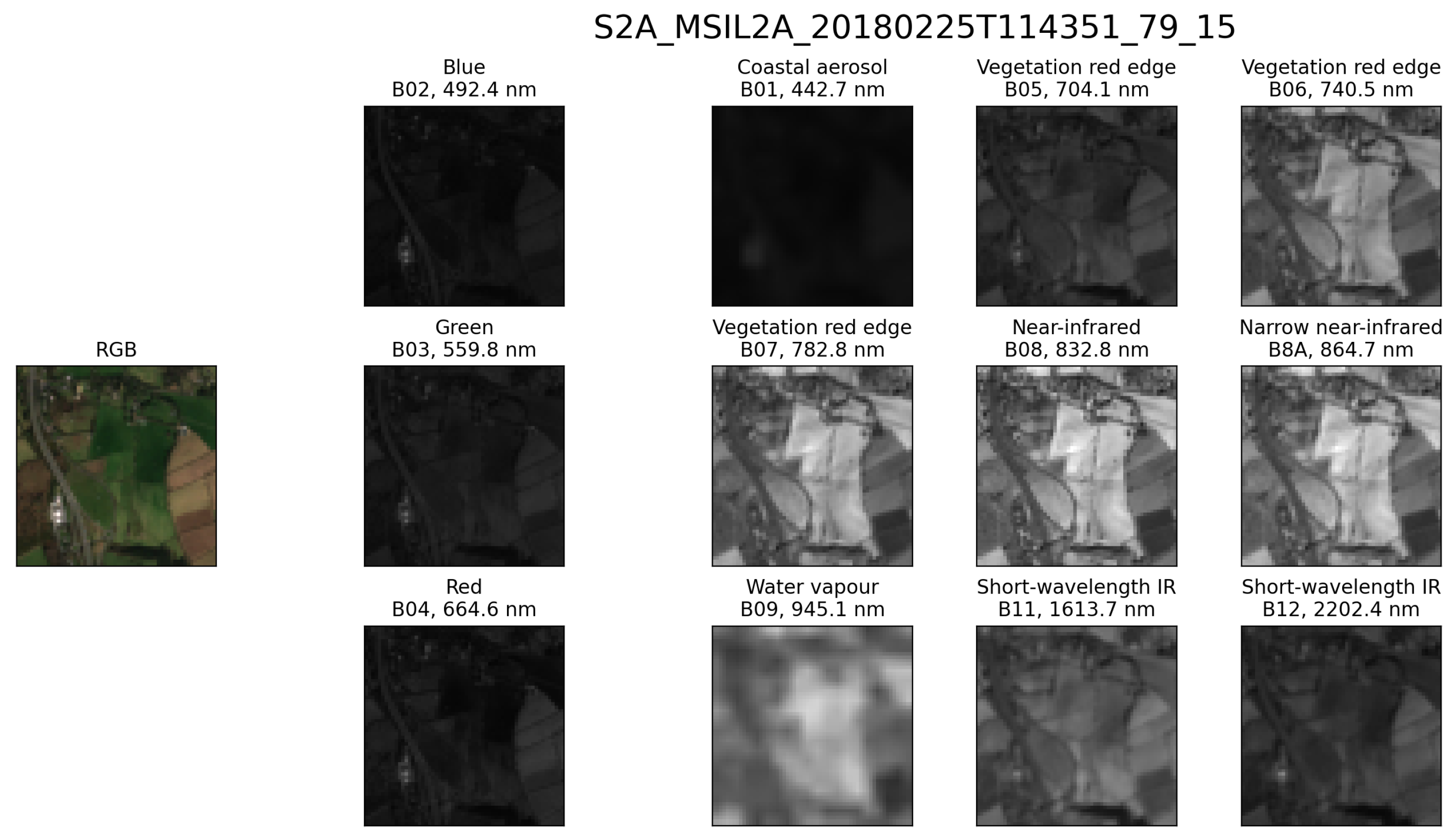
Figure 1 shows a multispectral image taken by the Sentinel-2 satellite [
8].
Many sensors for remote sensing capture multispectral images. However, they are more expensive than RGB cameras since the extended spectral information provided by these sensors requires additional complexity. The main application of multispectral reconstruction is the generation of multispectral images when this type of sensor is not available or when the only available images are RGB. In the case of having a mixture of RGB and multispectral images, multispectral reconstruction allows uniform processing. This can be important for change detection applications when part of the available images are RGB, and part are multispectral. Multispectral reconstruction can also be useful in applications that require multispectral image processing, but only RGB images are available. In this case, the spectral reconstruction could be considered as a preprocessing stage like that performed with filters and morphological or attribute profiles to highlight structures in the images. This spectral preprocessing could be useful in classification and object detection operations.
Therefore there has been considerable interest in developing algorithms for spectral reconstruction of multispectral images from RGB images. The goal of these algorithms is to minimize the error in the creation of multispectral images, achieving a result as faithful as possible to reality. The spectral reconstruction is a supervised machine learning problem, which requires a set of training images. Various techniques have been proposed, ranging from the use of functions or dictionaries [
9,
10,
11] to more innovative methods such as artificial neural networks [
12,
13,
14,
15,
16,
17,
18,
19,
20].
Early works of spectral reconstruction are based on the creation of dictionaries. Arad et al. [
9] construct a sparse spectral dictionary collecting images (either general or domain specific), whose projection into RGB provides a mapping between RGB atoms to hyperspectral atoms. Once all these components have been obtained, the spectral signature of each pixel of the test image was estimated using these dictionary representation applying the orthogonal match pursuit algorithm. A drawback of this method is that it treats each pixel independently, so the information available in the neighborhood of that pixel is not taken into account. This approach can be improved by adding additional information, such as the a set of spectral and convolutional features [
10]. Principal Component Analysis (PCA) has also been used to extract basis functions from collected databases of spectral reflectance [
11].
Architectures based on neural networks have been proposed in the literature for spectral reconstruction. Neural networks are capable of learning complex internal representations which allow them to extract the relevant features from the information they can process. Nguyen et al. [
12] addressed the problem with the use of radial basis functions. In this case, it continues to treat each pixel independently. In recent years, methods based on neural networks and deep learning have become more common [
21], especially by the use of Convolutional Neuronal Networks (CNNs). An advantage of CNNs is the automatic use of contextual information.
Different network types based on CNNs have been proposed for spectral reconstruction [
13]. A moderately deep (6 convolutional layers) model witch residual connections (ResNet) was proposed by Can et al. [
14]. The residual connections ensure that more features are available to the final layer. This approach was also used by Sharma et al. [
15], where the feature extraction from the three input RGB bands is done by a convolution layer, followed by 10 residual blocks for feature mapping. In addition, there have been studies of other convolutional neuronal network architectures, such as the U-Net used by Stiebel et al. [
16]. U-Net consists of a downsampling path and a upsampling path, which gives it the U-shaped architecture. During the contraction, the spatial information is reduced while feature information is increased. Residual connections during the expansion path complete the extracted features. Fubara et al. [
17] used a modified U-Net network with skip connections to allow lower level features to flow to deeper layers. Further, a second unsupervised learning method is proposed in that work, which would be useful in case there were no training images available.
Recently, the use of Generative Adversarial Networks (GAN) has been explored for solving a number of tasks in image processing. GANs consist of two networks, a generator and a discriminator. The generator tries to create new plausible synthetic data while the discriminator learns to discriminate between the training samples and the fake data. In this way, both networks improve their learning, the generator trying to trick the discriminator, and the latter trying to distinguish between real and fake data. Conditional Generative Adversarial Networks (CGAN) are an extension of the GAN where both the generator and discriminator are conditioned on some sort of auxiliary information such as class labels or data from other sources. CGANs have been proved useful for various applications in image processing, including classification [
22], denoising [
23], registration [
24], change detection [
25], information fusion [
26], and precipitation estimation [
27].
Isola et al. [
18] proposed using CGAN as general-purpose solution to image-to-image translation problems. These solutions include synthesizing photos from label maps, reconstructing objects from edge maps, and colorizing images, among other tasks. The proposed network in [
18] is a CGAN with a U-Net-based architecture as a generator and a convolutional PatchGAN classifier as a discriminator. Lore et al. [
19] used CGANs for RGB-to-multispectral image mapping, spectral super-resolution of image data, and recovery of RGB imagery from multispectral data. A similar solution was proposed by Alvarez et al. [
20] for spectral reconstruction. Since generator needs to yield full-size detailed images, a U-Net-like architecture was used. The discriminator was focused solely on modeling high-frequency structure and consists of a PatchGAN, which is simpler in terms of convolutional layer count. That is, the networks currently proposed in the literature for CGAN-based spectral reconstruction are built around of U-Net models as generators.
In this work we intend to expand the use of CGANs for spectral reconstruction by exploring other types of generators. Specifically, CNN, U-Net, and ResNet models are adapted and evaluated as generators in the CGAN. As training data for the CGAN, the BigEarthNet database [
28] have been used. This database contains approximately half a million images taken from the Sentinel-2 satellite, showing an aerial view of 10 European countries. The rest of the paper is organized into four sections.
Section 2 presents the methods used in this study, including the description of the proposed classification network. The experimental results for the evaluation in terms of classification performance and computational cost are presented in
Section 3. Then, the discussion is carried out in
Section 4. Finally,
Section 5 summarizes the main conclusions.
2. Neural Network Models
In this section we present the neural networks under study that are used as generators for a Conditional Generative Adversarial Network (CGAN) architecture. These networks are designed to convert the RGB composite image to a multispectral image of
n bands. The CGAN model for multispectral reconstruction is first described in detail and then the CNN, U-Net, and ResNet models, which are considered as generators. In
Section 3, variations in terms of layers, kernel size and skip connections are studied for these architectures.
2.1. CGAN Model
A generative adversarial network (GAN) is a class of machine learning framework where two networks (generator and discriminator) compete with each other. The generative network generates candidates while the discriminative network evaluates them. The objective of the generator is to synthesize candidates that the discriminator thinks are real, that is, to increase the error rate of the discriminator. The objective of the discriminator is to detect the candidates synthesized by the generator, this is to decrease its error rate. GANs provide an efficient way to learn deep representations with a relatively small number of training data. This is achieved by generating backpropagation signals through a competitive process that involves both networks. When the GAN is well designed, the generator and discriminator error rates are stable and balanced. The representations that can be learned by GANs may be used in a variety of applications, including synthesis, editing, superresolution, and classification.
Different models of GANs have been proposed in the bibliography, among which we can highlight [
29]:
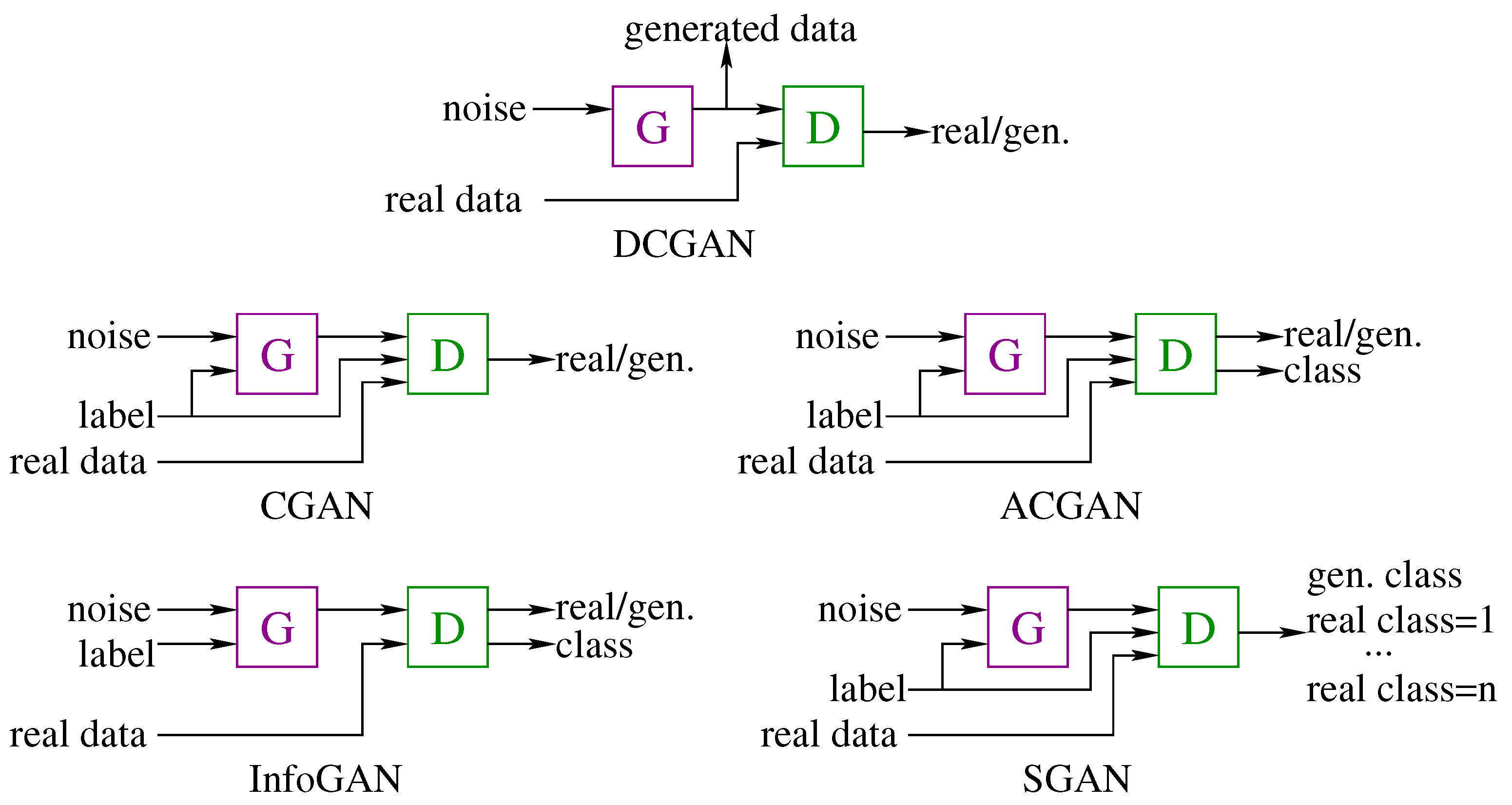
Deep Convolutional Generative Adversarial Network (DCGAN) [
30]. The DCGAN is the version of the GAN architecture which uses deep convolutional neural networks for generator and discriminator with a linked training between both networks. This architecture makes use of large unlabeled datasets to train the discriminator in order to be able to distinguish them from those synthesized by the generator. DCGAN has been used as the basis model for generating many other GAN models. For example, the discriminator model can be used as a starting point for developing a classifier, while the generator model could make use of additional information for generating the candidates.
Conditional Generative Adversarial Network (CGAN) [
31]. The CGAN is an extension to the GAN architecture that makes use of additional information as input both to the generative and the discriminative networks. In ordinary GAN, there is no control over modes of the candidates to be generated. In CGANs, additional information can be added as input to the generator in order to condition the synthesis of candidates. For example, if class labels are available they can be used. This labels can also be added to the discriminator input to help it distinguish generated candidates from real ones. By providing additional information, two benefits are achieved:
- –
Convergence will be stable and faster since the random distribution that candidates follow will have some pattern.
- –
The generator model can be used to generate candidates of a given specific type, for example, for a class label.
Auxiliary Classifier Generative Adversarial Network (ACGAN) [
32]. The ACGAN is an extension to the GAN architecture in which both the generative and the discriminative networks are class conditional as with the CGAN, but also adds an additional model to the discriminator to detect the class label. That is, the discriminator model must predict whether the given candidate is real or generated as in the CGAN, but also will predict the class label of the candidate.
Information Maximizing Generative Adversarial Network (InfoGAN) [
33]. The InfoGAN is an extension to the GAN architecture that introduces control variables that are automatically learned by the architecture and allow control over the characteristics of the candidate generated. For example, style, thickness, and type in the case of generating images of handwritten digits. This architecture is motivated by the desire to control and decouple the properties in the generated candidates. The InfoGAN involves the addition of control variables to generate an auxiliary model that predicts the control variables, trained via mutual information loss function.
Semisupervised Generative Adversarial Network (SGAN) [
34]. The semi-supervised GAN is an extension of the GAN architecture for training a classifier model while making use of labeled and unlabeled data. Semi-supervised learning is the challenging problem of training a classifier in a dataset that contains a small number of labeled examples and a much larger number of unlabeled examples. In the SGAN, the discriminator is modified to predict
classes, where
n is the number of classes in the classification problem and the additional class represents the synthesized candidate. It involves directly training the discriminator model for both the unsupervised GAN task and the supervised classification task simultaneously.
These GAN architectures are illustrated in
Figure 2. In this work, we have chosen the CGAN architecture, since it makes possible to add additional information to both generator and discriminator, which will help the generation of multispectral images. On the other hand, a classification of the candidates is not necessary for this task. In our case, the CGAN architecture makes it is possible to add a RGB composite image as input to the generator in order to synthesize the multispectral image, without requiring the classification of the results [
20]. In summary, the functions of generator and discriminator for the task considered are:
Generator: takes as input an RGB composite image, and its goal is to learn how to create the most realistic multispectral bands possible.
Discriminator: takes as inputs the RGB composite image and the multispectral bands synthesized by the generator. Its function is to determine if the multispectral bands are real or generated.
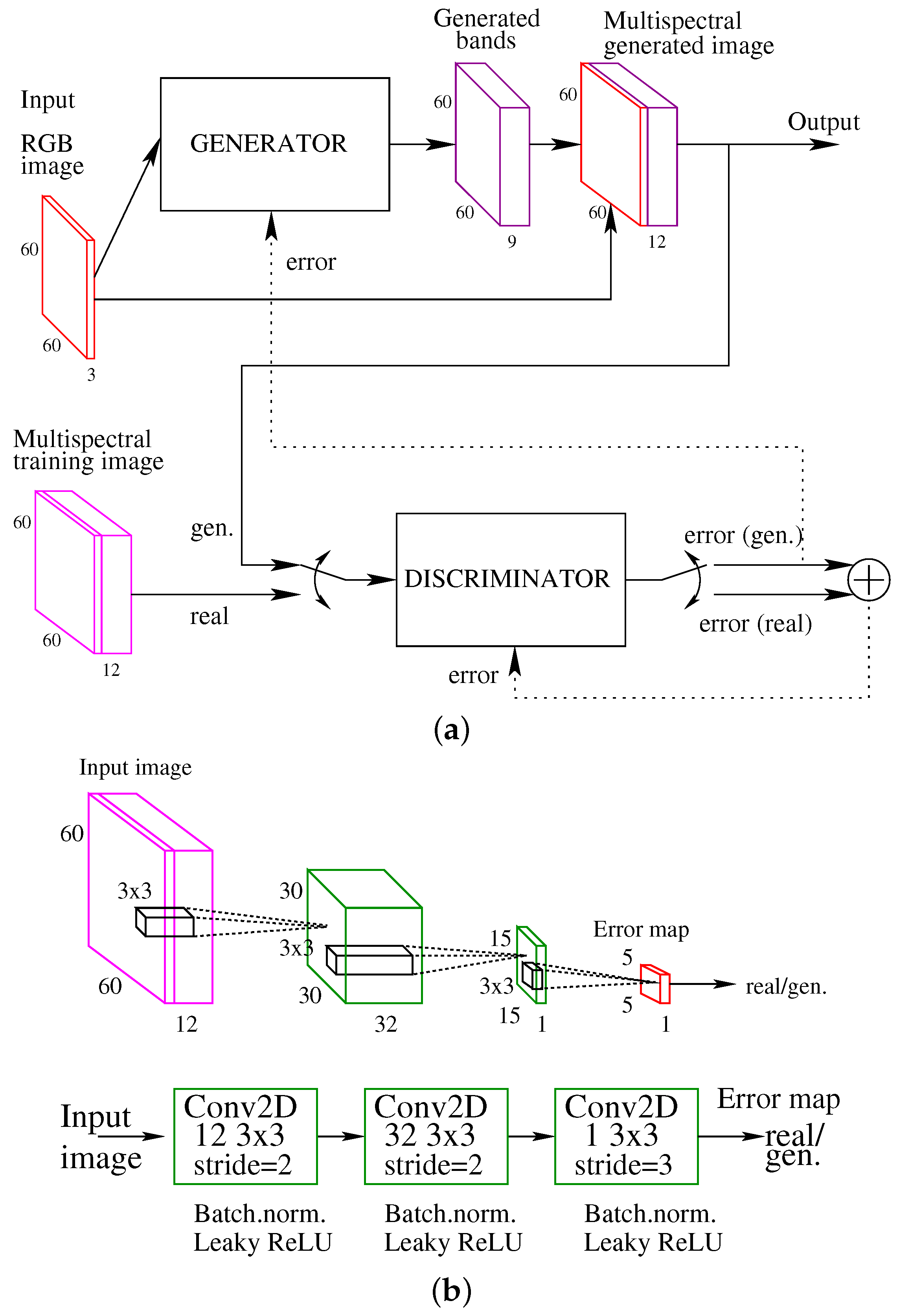
The CGAN architecture for spectral reconstruction is shown in
Figure 3a. The CGAN training process begins in the generator. The input to this part of the network is an RGB composite image, providing a multispectral image as output. Since the objective of the GAN is to synthesize the best possible multispectral image, the best effort should be put into the design of the generator. In this work, different types of networks (CNN, U-Net, and ResNet) have been considered as generator.
Then it is the turn for the discriminator to work. The discriminator takes as input the RGB bands and the multispectral bands of an image and provides a two-value output, which indicates whether the multispectral image is real or generated. In our CGAN, the discriminator is a classifier PatchGan. It uses convolutional layers, consisting of two convolution modules, batch normalization, and an activation function leaky ReLU, as can be seen in the
Figure 3b. A final convolution is applied to reduce the size of the result.
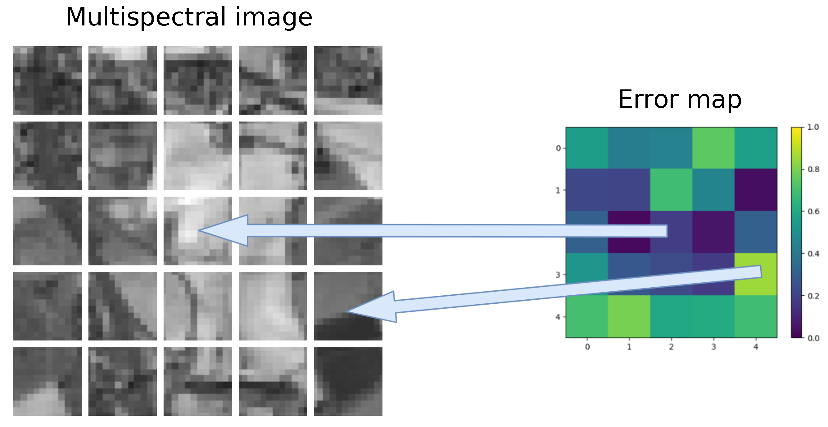
In more detail, the operation of the discriminator is as follows. The discriminator must detect whether the image structure is real or generated, and for this it computes an error map by subdividing the image into blocks [
18].
Figure 4 shows a example of error map of size
obtained from a image of size
pixels when using the discriminator of the
Figure 3b. Each component of the error map estimates the percentage the structure of a particular section of the image is real or generated. This operation is repeated twice, first with the pair RGB bands/multispectral bands provided by the generator, and then with a pair of RGB bands/multispectral bands from the training set. The function used to evaluate the obtained values and build the error map is binary cross-entropy. Finally, to combine the two error maps, the two values obtained by applying this function are added together. This value is what is used by the discriminator to learn to distinguish the generated images from the real ones.
The training of the generator uses another different error function, which takes in counts the result of the discriminator [
18]:
where
is the result of applying the binary cross-entropy function to the discriminator output taking as input the generated image,
is the average absolute error between the expected image and the generated image, and
as proposed by Isola et al. [
18] to reduce the visual artifacts that may be introduced on certain applications.
2.2. CNN Model
A Convolutional Neural Network (CNN) has mainly two layers: convolutional layers and pooling layers. In the convolutional layer, the convolution operation is applied several times using filters or kernels to obtain a map of features. These maps provide information about the content of the image. Several filters can be applied in the same layer and several feature maps will be created. The size of the filters may vary, and the most common are windows of size
and
. The pooling layer is responsible for extracting the most representative pixels in each subregion of an image. There are several types of subsampling operations. One of the most used is max pooling, that extracts the maximum value in each window [
35].
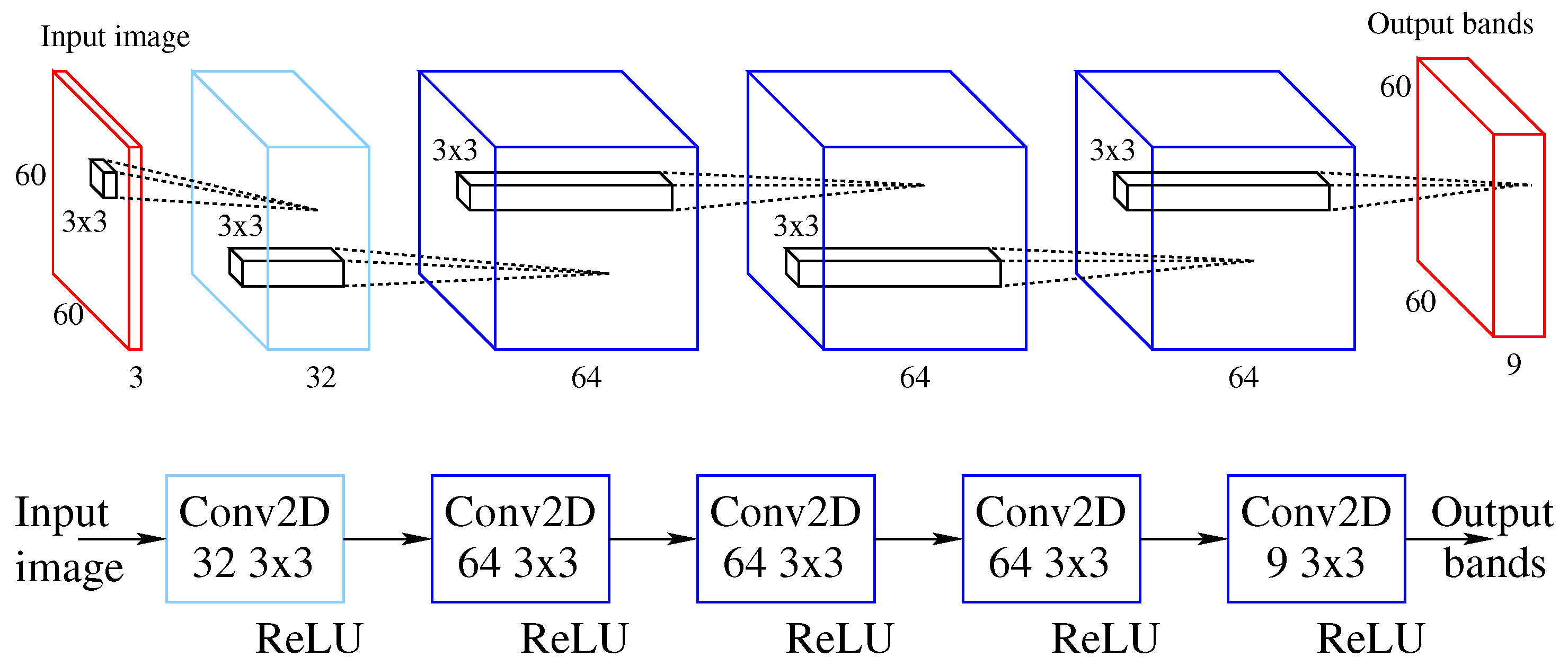
The CNN model considered in this work to integrate into a CGAN as a generator is designed using five convolutional layers. This network is illustrated in
Figure 5. The upper part of the figure shows the feature maps, while the lower part illustrates the operation that is carried out. The number of features increases to 64, while the dimension of the input image remains constant. The number of output features in the last layer can be adjusted to suit the number of spectral bands required. In this network, the number of output bands is set to 9, which added to the three original bands gives a total of 12. This is the number of spectral bands available in the images of the BigEarthNet database, details of which are presented in
Section 3.
The multispectral reconstruction is approached as a regression problem, so the use of pooling layers is removed as proposed by Stiebel et al. [
16]. These layers are used in classification problems, but in the case of reconstruction problems they would cause a loss of information.
This CNN model will be introduced as a generator within the CGAN. The resulting network will be evaluated and considered as a basic scheme with which to compare other more efficient generators.
2.3. U-Net Model
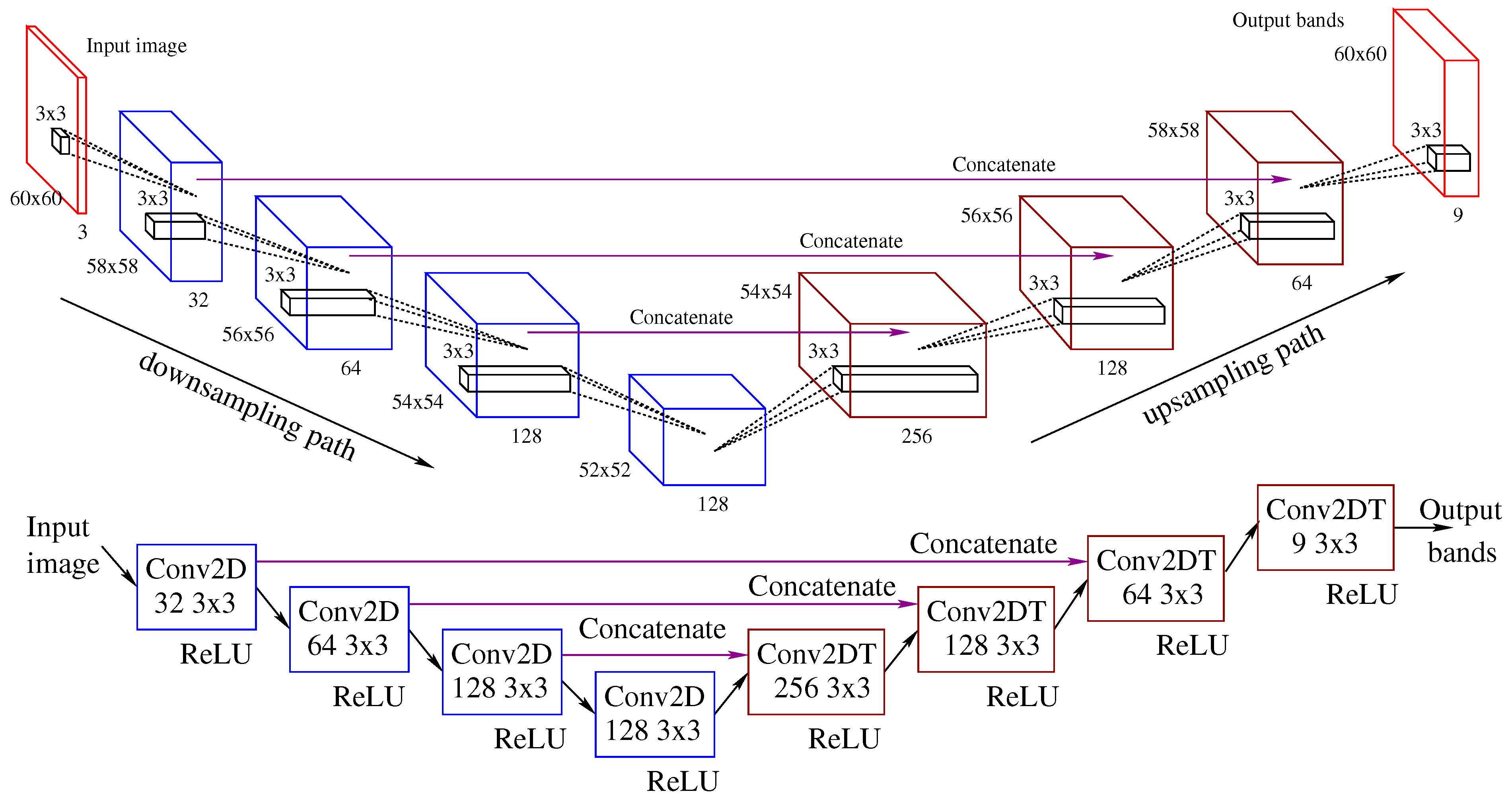
The U-Net architecture consists of a downsampling path followed by an upsampling path. A convolution operation is applied in the layers of the downsampling path, while a transpose convolution is used in the layers along the upsampling path. During the downsampling path, the spatial information is reduced based on the size of the kernel, but new features (in the spectral dimension) are created. The upsampling path performs the reverse function. The features of a transposed convolution are combined with the information of previous layers to produce a more precise spectral reconstruction. After passing through a layer, the spatial resolution increases.
Figure 6 shows the model considered in this work, that is based on the U-Net proposed by Stiebel et al. [
16]. The upper part of the figure shows the feature maps, while the lower part indicates the operation that is carried out. The network input is a RGB composite labeled as Input image in
Figure 6 while the output consists of the nine additional bands of the multispectral image, labeled as Output bands in the same Figure. The downsampling path is indicated by a downward arrow in the figure, and the upsampling path by an upward arrow.
Figure 6 also illustrates the skip connections and the operation done that combine the output of one layer in the downsampling path as the input to a layer in the corresponding upsampling level. In
Figure 6 the spatial dimension of the image is reduced by 2 in each layer in the downsampling path while the number of features progressively increases to 128 in the last layer of this path.
Figure 6 also illustrates in magenta the skip connections that combine the output of one layer in the downsampling path as the input to a layer in the corresponding upsampling level.
Since the U-Net proposed in [
16] was designed to operated independently and not included within a conditional GAN, in this work the U-Net will be adapted to operate as a generator within that architecture. The original U-Net architecture, proposed by Ronneberger et al. [
36] for biomedical image segmentation, will also be considered as a generator for the CGAN named U-Net_b. The U-Net_b model reduces by 2 the dimension of the images in each layer along the downsampling path and magnified it by this same factor along the upsampling path. This is the generator used in the CGAN of Alvarez et al. [
20].
2.4. ResNet Model
The Residual Neural Network (ResNet) architecture is characterized by using skip connections, which reduce the training error when adding more layers and solve degradation problems [
37]. The ResNet considered in this work is based on the residual network proposed by Can et al. [
14] for spectral reconstruction. Since the network was designed to operate independently and not included within a GAN, in this work the ResNet will be adapted to operate as a generator within CGAN.
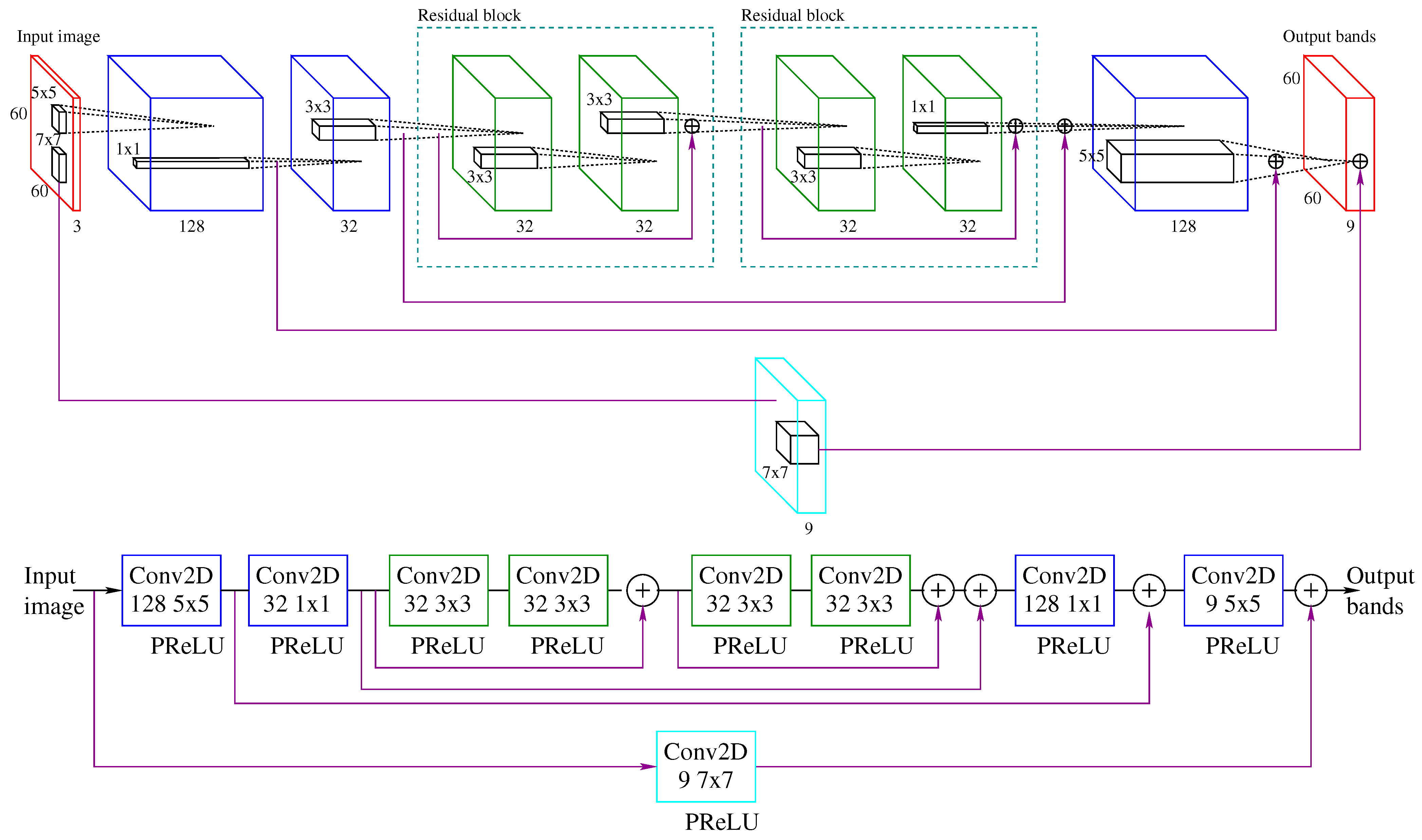
The ResNet model is shown in
Figure 7. The upper part of the figure shows the feature maps, while the lower part indicates the operation that is carried out. The boxes represent the convolutional layers, with the labels indicating the size of the kernel. The residual blocks are framed in dotted lines, while the lower lines connecting both sides of the network show the skip connections used in this architecture.
The backbone of the network has two residual blocks. The two convolutional layers before the residual blocks perform a feature extraction and a compression, respectively. Despite the initial features are shrunk, they are used through the skip connections in the last layers of the network. This structure has benefits in terms both of execution and performance, since compressing the features that follow the main path speeds up the computation time and reduces overfitting. The skip connection on the bottom side in
Figure 7 estimates the basic mapping from RGB to multispectral reconstruction by a
convolution layer [
14]. The last two convolutional layers expand the features to approximate the output to the multispectral image. Through the skip connections, the initial learned features are also used in the network.
Different than the original residual blocks introduced in [
37], a Parametric Rectified Linear Unit (PReLU) activation function is used in this work, instead of a ReLU as in the ResNet architecture proposed by [
38]. The PReLU function was shown to improve over the traditional non-parametric ReLU. Other possible modifications to this network to optimize its operation as a generator within the GAN are discussed in
Section 3.
Table 1 includes the network models considered as generators for a CGAN.
3. Results
In this section, the accuracy of the multispectral image reconstruction and the computational cost of the CGAN are evaluated using as generators the CNN, U-Net, and ResNet neural networks designed in the previous section. The CGAN of Alvarez et al. [
20] that uses the U-Net of Ronneberger et al. [
36] as generator is also included in the analysis, named U-Net_b in this section. It was adapted removing the PatchGAN layer in the discriminator and reducing the number of layers and filters to fit the input image size.
Table 1 includes those networks and key parameters.
The BigEarthNet [
28] dataset was used for training the CGAN. In this work 10,000 image patches were used for the experiments. The size of the dataset was analyzed prior the experiments, considering the limitations of the available hardware. The experiments were carried out on a personal computer with a AMD Ryzen 5 2600 CPU at 3.4 GHz with 16 GB of RAM, and a GPU NVIDIA GeForce GTX 1660 at 1.7 GHZ with 6 GB of RAM. The code was written in Python using the TensorFlow library [
39] under a Linux operating system.
The multispectral reconstruction was evaluated using the Root Mean Square Error (RMSE). The RMSE measures the amount of error between the reflectance value of the image and the predicted value. Since it is an error measure, networks that obtain a lower RMSE provide a more accurate reconstruction. The RMSE retains the same scale as the data, so the ranges can be transformed to a common scale so that the results can be compared. The computational cost was measured in terms of execution time (t) and the performance between the CPU and GPU was compared in terms of speedup as the fraction .
3.1. Dataset
The BigEarthNet [
28] dataset has approximately half a million of multispectral images patches taken from 125 high resolution images acquired by the Sentinel-2 satellite. All the tiles were atmospherically corrected by the Sentinel-2 Level 2A product generation and formatting tool (sen2cor) [
28]. Sentinel-2 carries an optical instrument payload that samples 13 spectral bands: four bands at 10 m, six bands at 20 m and three bands at 60 m spatial resolution. The spectral band B10 was discarded as it does not contain information of the surface because of the sen2cor processing methodology.
Table 2 shows the details of the multispectral patches. As the image patches have different resolution at different wavelengths, all the spectral bands were downscaled to 60 × 60 as it is the most common size among all bands, except bands B01 and B09 that were upscale to 60 × 60. See
Table 2 for details of the patch sizes.
For the experiments, 10,000 patches were randomly selected from the BigEarthNet dataset and divided into three non overlapping sets: 80% was used for training and validating and 20% for testing. Of the total samples for training and validation, we make the same partition with 80% for training the neural networks and 20% for validate the performance during the training. Thus, 64% of the total number of samples was used for training, 16% for validation and 20% for testing.
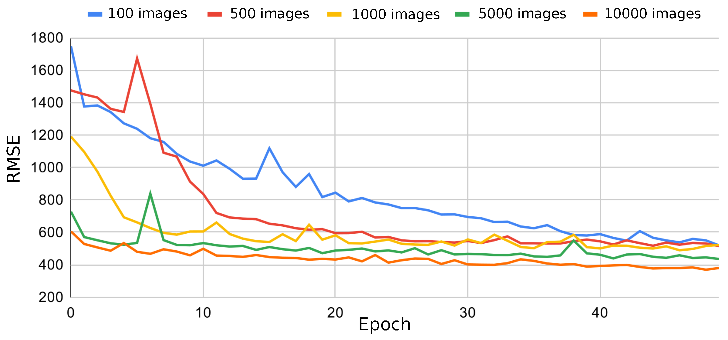
Figure 8 shows the RMSE during the training for a ResNet using different number of patches. It is observed how the error decreases when a larger number of patches is used, so the available RAM in the computer was the limiting factor for the dataset size. As our GPU has only 6 GB of RAM compared to the 16 GB of RAM for CPU memory, 10,000 images were used in the experiments. Each image needs 168.75 kB (4 bytes × 60 × 60 × 12), that is the size in bytes of each spectral band times the number of bands plus additional information from the metadata and software used for the experiments.
3.2. CGAN Generators Comparison
To evaluate the CGAN with different networks as generators (CNN, U-Net, U-Net_b [
20,
36] and ResNet), these networks were first trained individually using the validation set and different parameters in order to set up the configuration of each model.
3.2.1. Configuration of the Neural Networks as Generators
To obtain the best results for each network operating as a CGAN generator, some variations and optimizations in the configurations were studied. These variations are numbered from 1 to 4 in
Table 3. The first column lists the variations for the U-Net architecture and the second column lists the variations of the ResNet. The row marked with ‘0’ indicates the base architecture on which the variations are applied. The networks were trained for 200 epochs at a learning rate of 0.001.
Regarding the U-Net, the following modifications were studied: (1) variation of the number of layers, (2) add a preprocessing layer for noise images, (3) variation of the size of the convolutional filters, and (4) replace the function concatenate by the add function. Best results were obtained for the configuration shown in
Figure 6: a
convolution filter with no padding, a ReLU activation function and concatenated skip connections. The main reasons are that a small convolution filter adds information from the nearest neighbors that may have more similarity and the concatenation activation function keeps all information in the skip connections while the add function means losing some information.
Regarding the ResNet, the following modifications were considered: (1) variation in the number of filters in the convolutional layers, (2) variation in the number of residual blocks, and (3) variation in the number of paths. After analyzing the results we can conclude that adding residual blocks or doubling the number of filters marginally improves the results. However, in practice, these two modifications are not recommended, as the computing time they need to train is twice as long, and we only get an improvement of less than 1%. On the other hand, it has been verified that the 2 paths of the proposed architecture are useful and reduce the error by 4% without increasing the execution time. Best results were obtained for the configuration shown in
Figure 7: two residual blocks and two paths.
3.2.2. Configuration of the CGAN
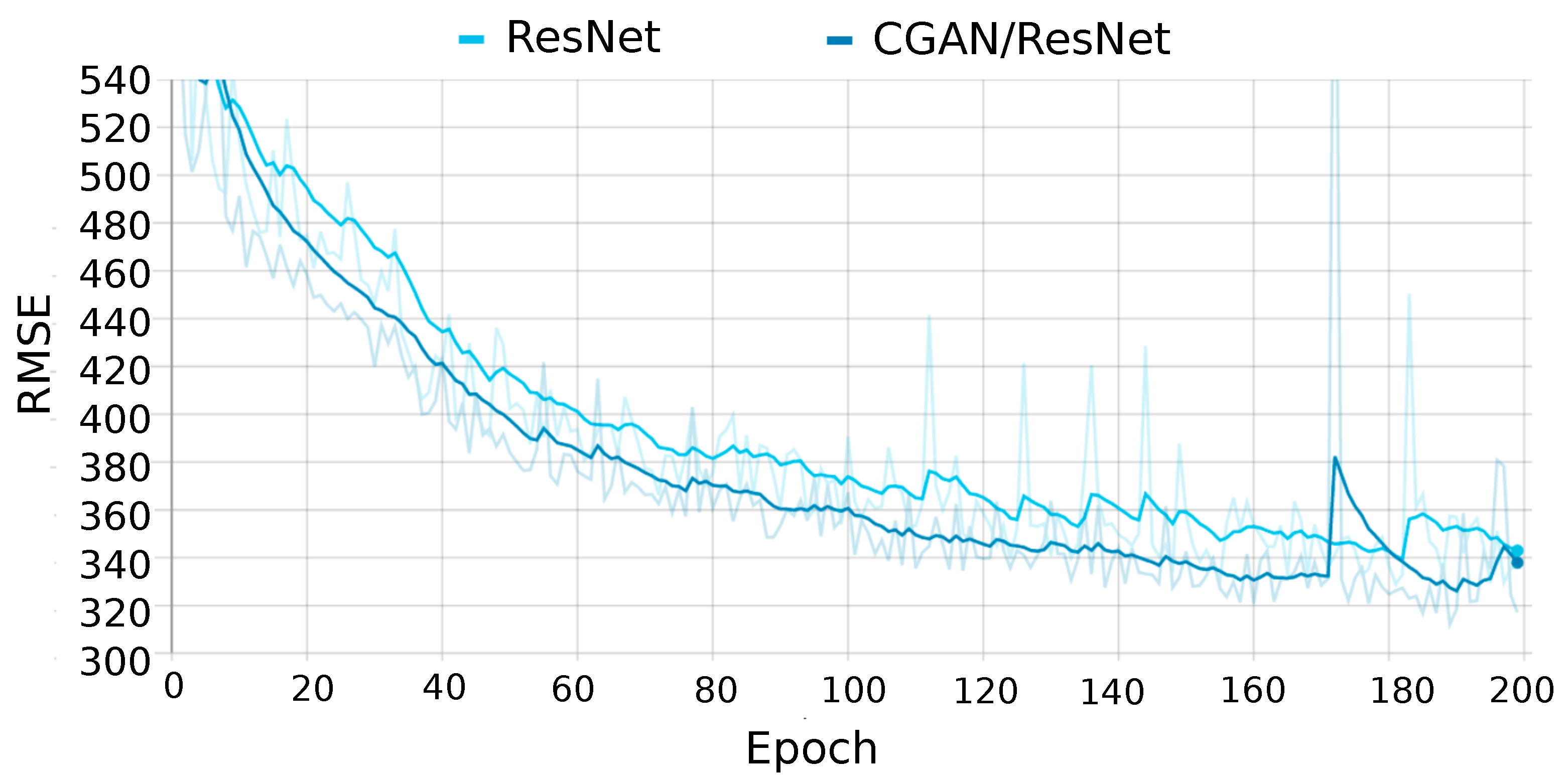
Next, we proceed to evaluate the CGAN by integrating the above networks as generators. As previously mentioned, CGAN learning is based on competition between the two networks that compose it. This learning method makes CGAN provide better results than other networks even when they are included in CGAN as part of its architecture, as shown in
Figure 9. In this figure, the CGAN using a ResNet as a generator is compared to the standalone ResNet. During most of the training, the error rate of the CGAN is lower than that of the ResNet. A validation set of 1600 images was used to plot the error during the training phase.
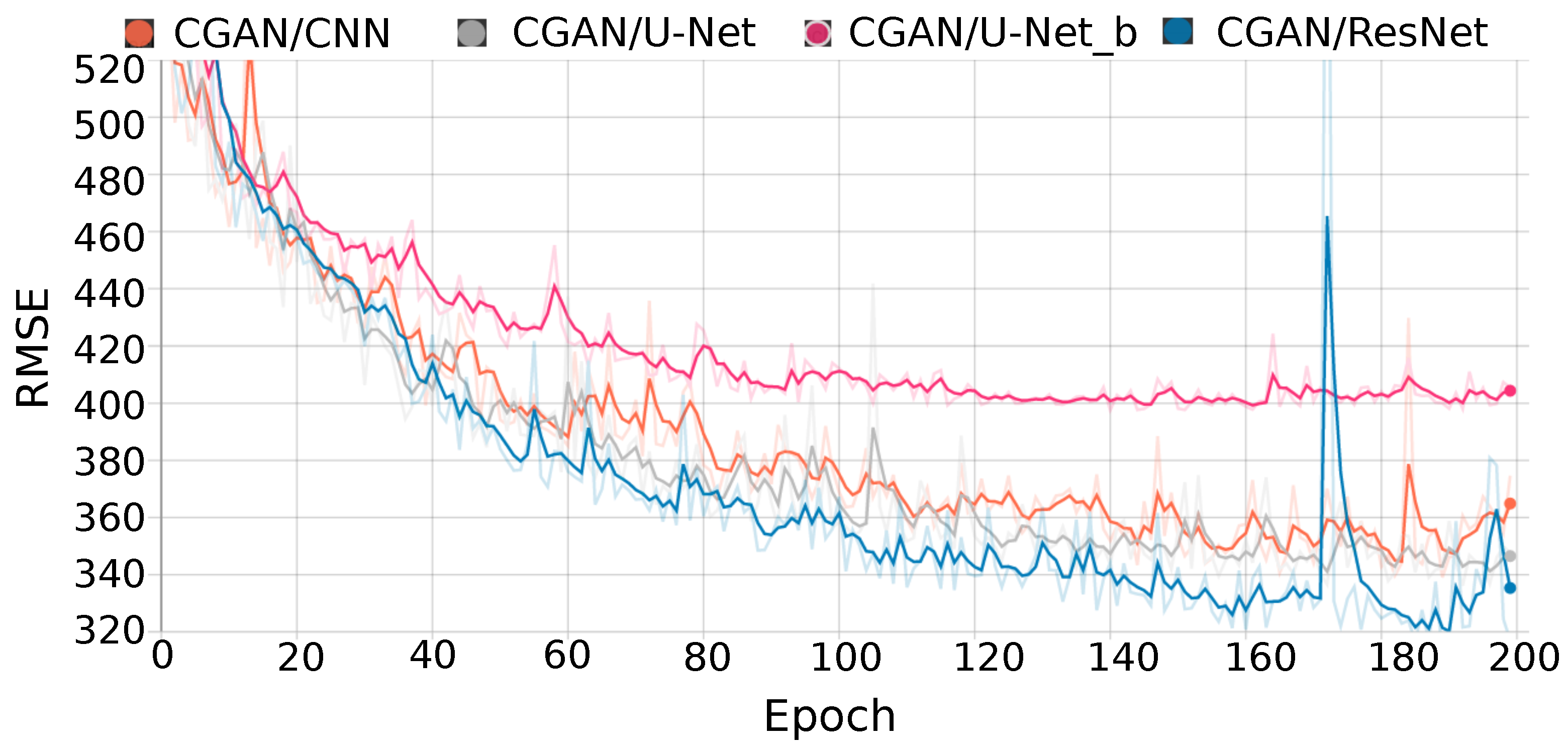
Figure 10 shows the RMSE obtained during the training of the CGAN for the four generators during different number of epochs. It can be observed that for the CGAN with U-Net_b as a generator (denoted by CGAN/U-Net_b) the validation error remains constant from 100 epochs, while for the CGAN with CNN, U-Net and ResNet the validation error decreases for almost 200 epochs, reducing the overfitting. The validation set, consisting of 16% of the images, was used for this study.
With the configuration extracted from the training step, the CGAN was evaluated for the multispectral reconstruction calculating the RMSE on the entire test set. The error was calculated from the histogram of the entire dataset using a common scale, resulting a range of values from 0 to 16,384.
Table 4 shows the reconstruction error (RMSE) for each network, the number of passes of the entire training dataset (epochs), the execution time for training on CPU and GPU, as well as the GPU speedup with respect to the CPU execution time. The CGAN with ResNet has the best reconstruction result with an error of 316. The CGAN with U-Net_b got the highest error with a RMSE value of 404, while for CNN and U-Net a similar accuracy in the reconstruction is obtained, in particular, an error of 363 and 354, respectively.
Regarding the execution time for training, the CGAN with ResNet needs 62 min when using the GPU, while for CNN and U-Nets it needs less training time. The CGAN with U-Net_b is the one that needs the least time (11 min), while for U-Net it needs 49 min, both using the GPU. From
Table 4 it is also observed that all networks achieved an increase in speed when using the GPU. For the CNN and U-Net the speedup is higher, reaching almost 15×. Both networks, compared to U-Net_b and ResNet are better suited for GPU execution. The speedup obtained on GPU is 9.6× for the ResNet and 2.2× for the U-Net_b.
3.3. Multispectral Reconstruction Comparison
Based on the best results obtained with the CGAN using the ResNet as a generator, in this section we compare the multispectral reconstruction from RGB images with two real multispectral images: an image with pastures and an image of the ocean, see
Figure 11 and
Figure 12, respectively. These figures shows an error map as the absolute error between the each spectral band of the real multispectral image and the reconstructed image. These error is calculated between 0 and 1. In addition, the RMSE calculated for each spectral band is also included in those figures.
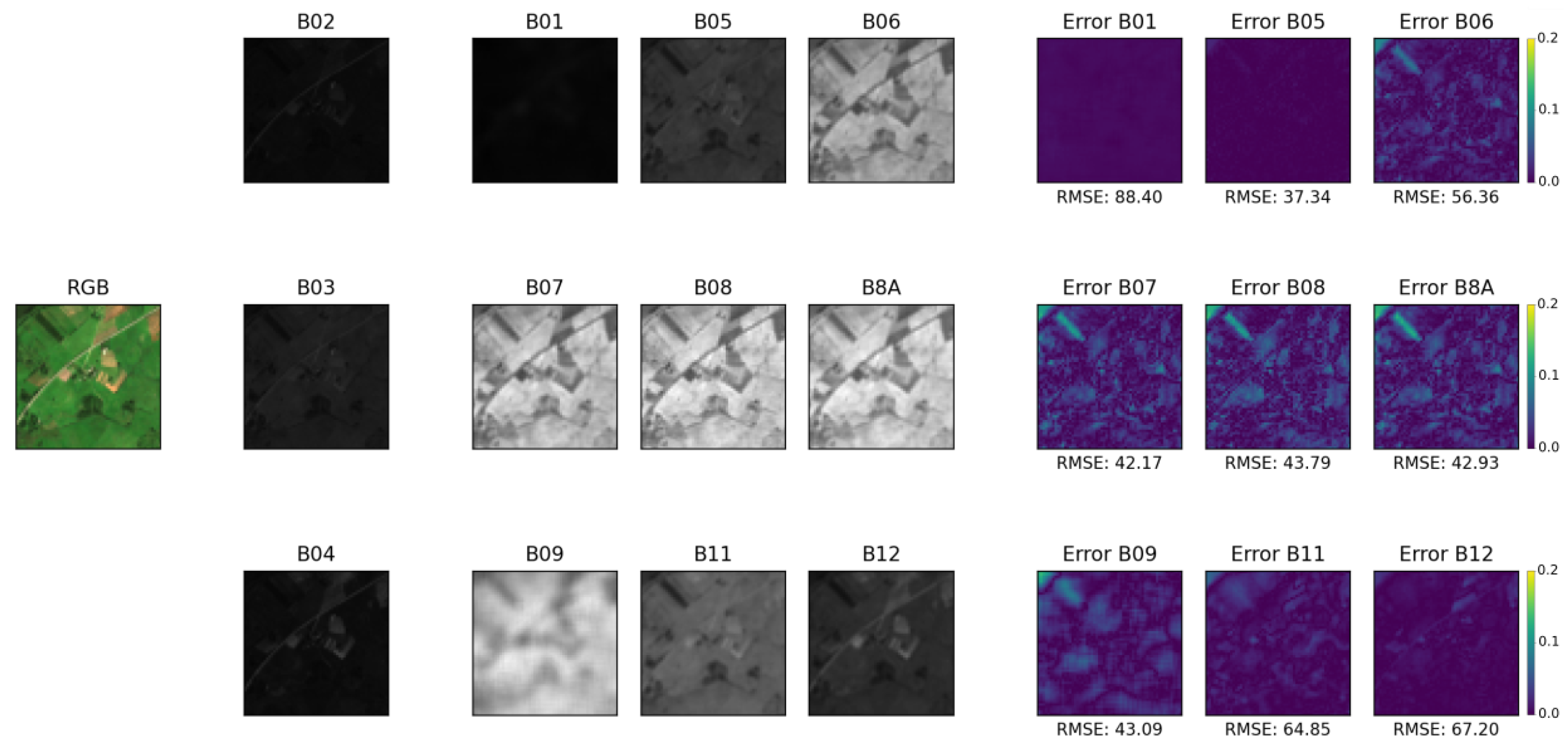
Figure 11 and
Figure 12 consist of several sections. On the left, the RGB composite is shown and the next column presents the red, green and blue channels which are the input of the neural network. The next three columns shows the rest of spectral bands of the image (see
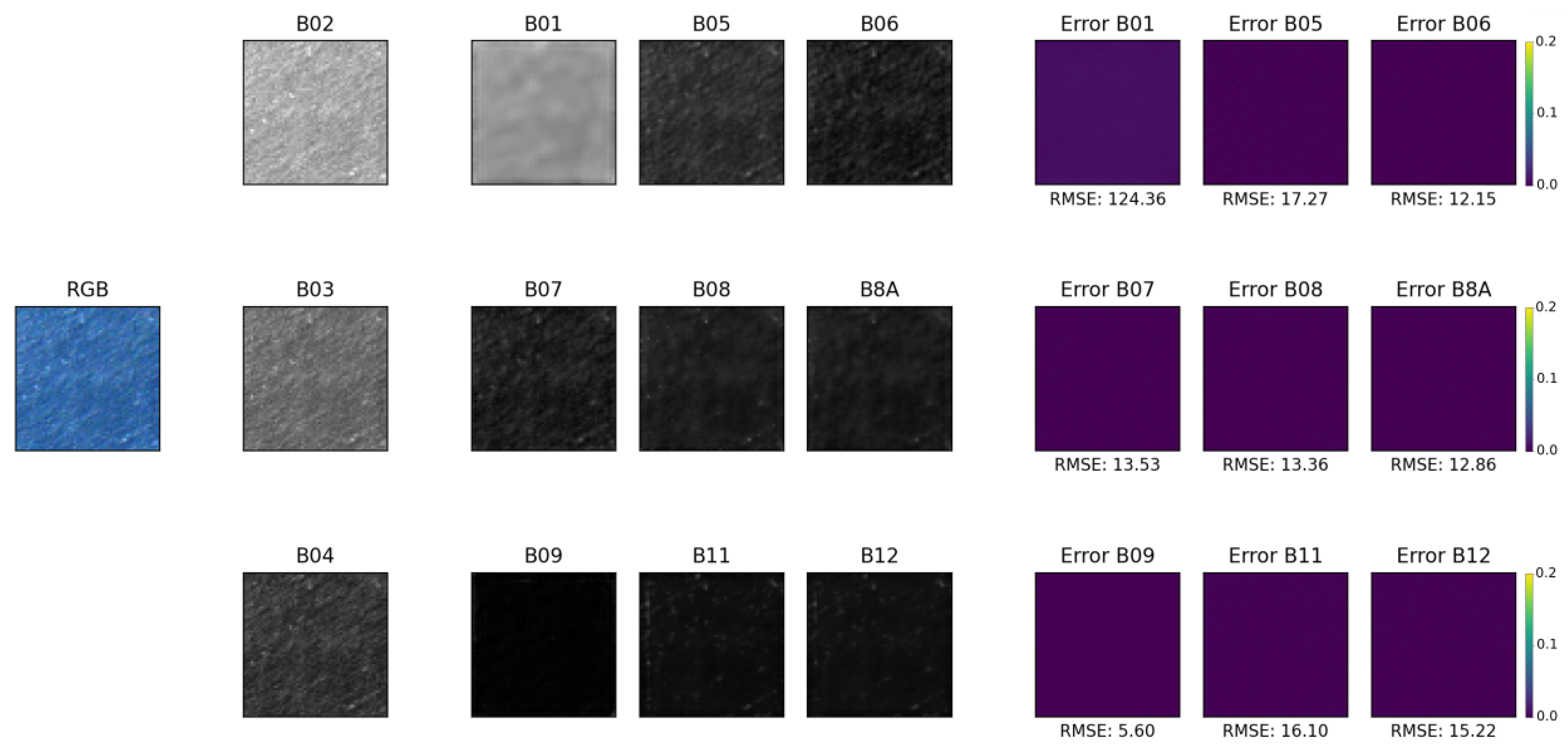
Table 2 for details of the name and number of bands). These nine bands are the output of the neural network. Finally, the last three columns are the absolute error that results from comparing the generated bands with the real ones. To improve the visual inspection of the error, the scale has been adjusted between 0 and 0.2 in these figures since no error in the bands exceeded that value.
Taking a closer look at
Figure 11 (pasture image), the RMSE is under 100 in a range of values from 0 to 16,384, for all the spectral bands but it is observed in the top left of the image a parcel of forest in the middle of the pastures that represent the higher error (higher intensity) in the error map. In the image of the ocean, a minor error is observed, below 20, except in B01, which is greater than 100. As explained in
Section 3.1 the spectral band B01 was upscaled to 60 × 60. Since upscaling makes the image patch looks blurry and have a lower quality for the neural network a higher RMSE is expected for these spectral band.
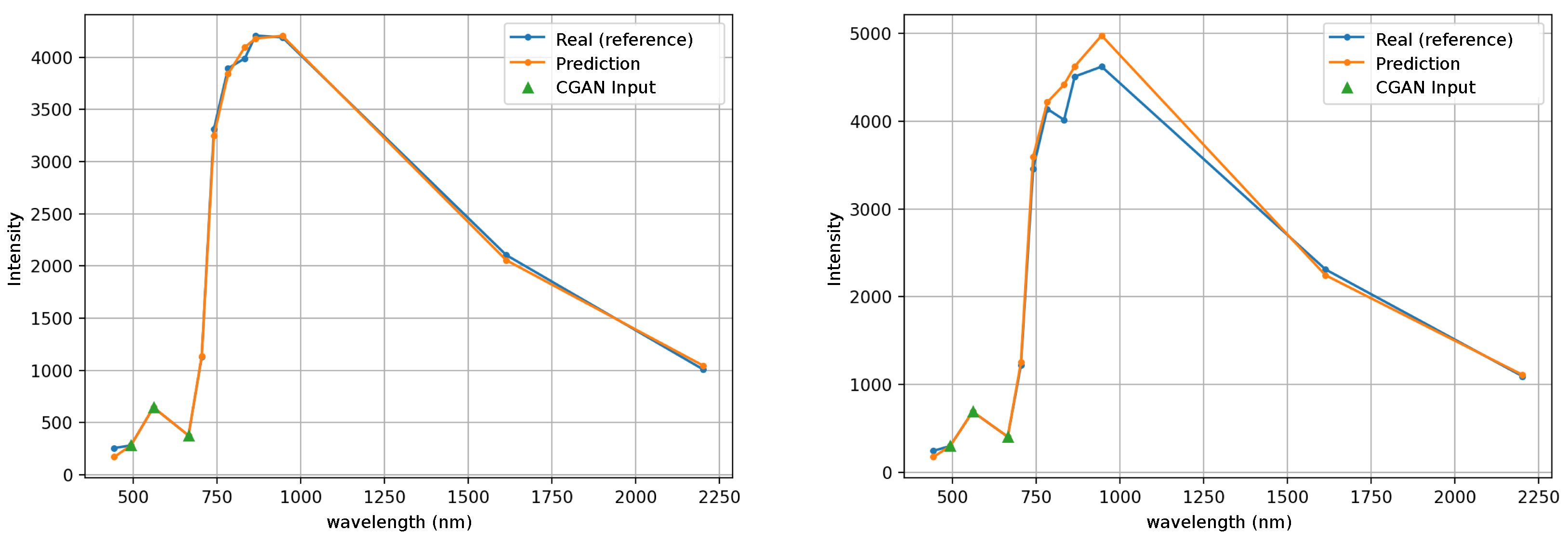
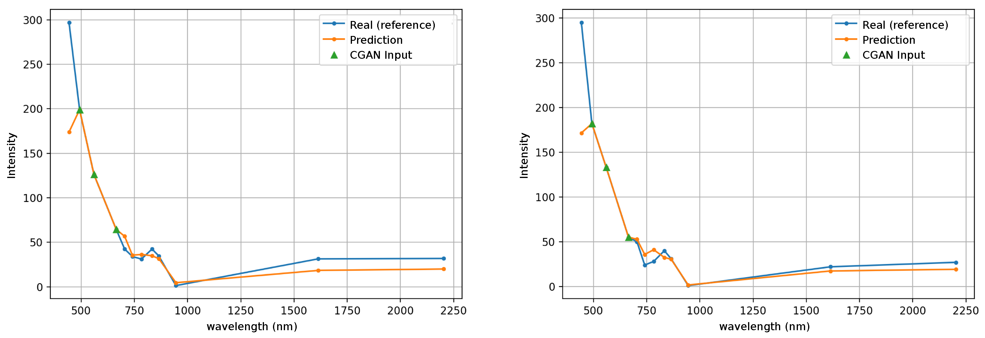
The average intensity of the pixels was also compared as illustrated in
Figure 13 for the pasture image and
Figure 14 for the ocean image. For each band, the average value is calculated and it is plotted in the left graph of these figures. The right graph shows a random pixel of the image. The average intensity has a very good match for the image of pasture, see
Figure 13 (left), and a slight difference for the ocean image, see
Figure 14 (left), especially in the first band (443 nm), which is the spectral band with the highest RMSE, as shown in the previous section. The difference between the real multispectral image and the reconstruction one is best appreciated when selecting a random pixel. In
Figure 13 (right) it is observed between bands B06 (741 nm) and B09 (945nm). In the ocean image, see
Figure 14 (right), the difference is also in the vegetation red edge range from 704 nm to 783 nm. The details of the wavelengths and name of the bands can be seen at
Table 2.
4. Discussion
In view of the results obtained in this work, the problem of generating multispectral images from RGB images can be achieved with sufficient quality using CGAN models. The RMSE measured in a range from 0 to 16,384 was on average 316 using the ResNet generator on a set of 2000 test images. The combination of contextual information when using convolutional networks, a training with CGAN that prioritizes that the structure of the image is correct through the combination of a generator and a discriminator, and the use of a ResNet model as a generator, which reduces overfitting and allows training for more periods are the result of the study carried out in this work.
A limitation of deep-learning methods based on supervised learning as the one designed in this work is that they require training samples. In the same way as in supervised classifiers, which require training with the same types of materials (classes) that are to be classified in the images, the CGAN training must be carried out with samples of materials that will be present in the images to be reconstructed. In this sense, the presence of materials with which the deep learning network has not been trained would produce an indeterminate output. This does not imply that the reconstruction should be limited to images with a relatively homogeneous part of surface (forests, crops, etc.), but that all the materials included in the image to be reconstructed must be present during training.
In general, these limitations also apply to anomaly analysis, which is of great interest in many applications, e.g., in the detection of areas with plant damage for agriculture or ecological monitoring. However, in some cases this analysis may be feasible without specific training. For example, when the ground cover has intermediate levels of vegetation, ranging from bare soil to leafy vegetation. Like a supervised classifier, the spectral reconstruction network should be able to correctly handle these intermediate cases.
Fortunately, very extensive land cover databases are now available to facilitate the learning of deep-learning networks. The BigEarthNet database [
28], which contains approximately half a million images taken from the Sentinel-2 satellite, showing an aerial view of 10 European countries provide an ideal scenario for machine learning. Although this work focuses on the Sentinel-2 satellite, the database also provides images from the Sentinel-1 satellite. In addition, it is a database of public access. The use of this dataset in this work serve as a starting point for future contributions and improvements since it establishes a baseline of the results that can be achieved with the neural network architectures studied in this work.
In certain processing chains, the spectral reconstruction can be included as an additional step (generation of the multispectral images on basis of RGB images). In this cases, multispectral reconstruction could be considered as a preprocessing stage like that performed with filters and morphological or attribute profiles to highlight structures in the images. For example, this spectral preprocessing could be useful in classification and object detection operations. One advantage that spectral reconstruction networks have over classifiers is that their operation is completely automatic. In classifiers, images have to be labeled manually, often at the pixel level, which is labor-intensive and error-prone, in some cases requiring field views. On the contrary, the CGAN training is carried out automatically since it is a regression and both the input and output are obtained from the databases. In this way, spectral processing operations are decoupled from classification operations in the processing chain, with the advantages of massive training that the former have, since labeled images are not required.
With respect to CGAN models such as the ones used in this work, they can present some disadvantages. First of all, they require a lot of computational resources. For example, training the CGAN with a ResNet as a generator requires 62 min on the GPU of a commodity PC. However, the training is performed only once, while the inference operations are much faster (they require only one epoch compared to 200 during training). On the other hand, the design of CGANs is difficult. If the two networks that make up the CGAN, generator and discriminator, are not well balanced, the model will not reach convergence during training. Therefore, a careful study of the details of the networks is required to achieve effective designs.
5. Conclusions
The generation of synthetic multispectral images from color images offers the possibility of increasing the volume of images in datasets that can be used for supervised training, for example for classification of the Earth’s surface. These synthetic images must be generated with sufficient quality to be useful.
In this article a study and comparison of generators for Conditional Generative Adversarial Networks (CGANs) applied to multispectral image reconstruction from RGB images in remote sensing was presented. Among the CNN, U-Net and ResNet generators under study, the ResNet obtained better results in terms of Root Mean Square Error (RMSE). It was also possible to train the network for more epochs, avoiding the overfit that occurs in other proposals using a U-Net. The discriminator used in all CGAN models was a PatchGan classifier.
The runtime was also analyzed, showing that the U-Net and ResNet generators consume more time. Despite the experiments were executed using the computational capacity of a GPU, the training time of the model using the ResNet was 1 h and 2 min. However, the inference operation from RGB to multispectral was only a few seconds.
The study was carried out in a public database of multispectral images, the BigEarthNet database. The wide range of images of the Earth’s surface available in this dataset were of interest to generalize the training. Being an open access database, it is possible to establish a baseline of the results that can be achieved with the neural network architectures studied in this work.
As future works, the influence of different discriminators on the ResNet generator can be studied. It is also of interest to dive into the ResNet architecture to improve the execution time as other authors have done in the use of U-Net when it is used into a CGAN network. These future works could be executed on a high performance computing server with a GPU with more RAM, giving the possibility to use the entire dataset.


