Article

Precise Crop Classification of Hyperspectral Images Using Multi-Branch Feature Fusion and Dilation-Based MLP

1
Heilongjiang Province Key Laboratory of Laser Spectroscopy Technology and Application, Harbin University of Science and Technology, Harbin 150080, China
2
Department of Computer Science, Chubu University, Kasugai 487-8501, Japan
*
Author to whom correspondence should be addressed.
Remote Sens. 2022, 14(11), 2713; https://doi.org/10.3390/rs14112713
Submission received: 23 April 2022 / Revised: 31 May 2022 / Accepted: 4 June 2022 / Published: 5 June 2022
(This article belongs to the Special Issue Recent Advances in Processing Mixed Pixels for Hyperspectral Image)

Abstract

:
The precise classification of crop types using hyperspectral remote sensing imaging is an essential application in the field of agriculture, and is of significance for crop yield estimation and growth monitoring. Among the deep learning methods, Convolutional Neural Networks (CNNs) are the premier model for hyperspectral image (HSI) classification for their outstanding locally contextual modeling capability, which facilitates spatial and spectral feature extraction. Nevertheless, the existing CNNs have a fixed shape and are limited to observing restricted receptive fields, constituting a simulation difficulty for modeling long-range dependencies. To tackle this challenge, this paper proposed two novel classification frameworks which are both built from multilayer perceptrons (MLPs). Firstly, we put forward a dilation-based MLP (DMLP) model, in which the dilated convolutional layer replaced the ordinary convolution of MLP, enlarging the receptive field without losing resolution and keeping the relative spatial position of pixels unchanged. Secondly, the paper proposes multi-branch residual blocks and DMLP concerning performance feature fusion after principal component analysis (PCA), called DMLPFFN, which makes full use of the multi-level feature information of the HSI. The proposed approaches are carried out on two widely used hyperspectral datasets: Salinas and KSC; and two practical crop hyperspectral datasets: WHU-Hi-LongKou and WHU-Hi-HanChuan. Experimental results show that the proposed methods outshine several state-of-the-art methods, outperforming CNN by 6.81%, 12.45%, 4.38% and 8.84%, and outperforming ResNet by 4.48%, 7.74%, 3.53% and 6.39% on the Salinas, KSC, WHU-Hi-LongKou and WHU-Hi-HanChuan datasets, respectively. As a result of this study, it was confirmed that the proposed methods offer remarkable performances for hyperspectral precise crop classification.

1. Introduction

Hyperspectral imaging instruments can capture rich spectral signatures and intricate spatial information of observed scenes [1]. Plentiful spectral signatures and spatial information of hyperspectral images (HSIs) offer great potentials for fine crop classification [2,3] and detection [4,5]. Therefore, hyperspectral remote sensing can obtain the spectral characteristics and their differences more comprehensively and meticulously than panchromatic remote sensing [6]. Therefore, this paper uses hyperspectral techniques to finely classify crops and to promote the development of specific applications of hyperspectral techniques in agricultural remote sensing, such as monitoring the development of agriculture and optimizing the management of the agricultural industry.
Many methods have been applied to hyperspectral image classification in recent years. Early-stage classification methods are support vector machine (SVM) [7], random forest (RF) [8], multiple logistic regression [9] and decision tree [10], which can provide promising classification results. What is more, these classification methods can only extract the shallow feature information of hyperspectral images, which have limited ability to handle the highly nonlinear HSI data and limit the further improvement of their classification accuracy.
Recently, deep learning-based models have also been extended to HSI classification. In [11], Chen et al. used a deep stacked auto-encoder (SAE) to extract features from the spectral domain for HSI classification tasks. In [12], Tao et al. introduced a modified auto-encoder model, called multiscale sparse SAE, to construct two variants of feature-learning procedures for sparse spectral feature learning and multiscale spatial feature learning from unlabeled data in HSIs. Sun et al. proposed a hybrid classification method combined deep belief network (DBN) with principal component analysis (PCA) to improve the HSI classification performance [13]. Chen et al. introduced the Convolutional Neural Network (CNN) into HSI classification in [14]. In this paper, a regularized deep feature extraction (FE) method is presented for HSI classification using CNN. Zhang [15] proposed a novel spatial residual block combined parallel network, which extracted rich spatial context information to improve hyperspectral classification accuracy. Kanthi et al. [16] proposed a new 3D deep feature extraction CNN model for HSI classification in which the HSI data are divided into 3D patches and fed into the proposed model for deep feature extractions. Zhang et al. [17] proposed a multi-scale dense network for HSIs, which can extract more refined features and make full use of multi-scale features. Zhu [18] proposed a self-supervised contrastive efficient asymmetric dilated network for HSI classification, which designed a lightweight feature extraction network EADNet in the contrastive learning framework.
While CNN-based models have yielded positive scores in HSI classification, the complexities intrinsic to remote-sensing hyperspectral images retain limitations concerning the performance of numerous CNN models. First, the parametrization of CNNs multiplies as convolution layers multiply exponentially and becomes larger as the computational capabilities rise. Additionally, the computational has turns into a bottleneck for practical implementations due to the long runtime of multiplication and summation. Lastly, the translation invariance and local connectivity of CNNs can interfere with the effectiveness of HSI classification.
MLP, as a neural network with fewer constraints, can eliminate the adverse effects of local connectivity and focus on spatial structure and information. It has been proved to be a promising machine-learning technology. Ilya [19] proposed an architecture based on MLP, including channel-mixing MLPs and token-mixing MLPs. However, the MLP-Mixer can achieve performance comparable to CNN. Yu [20] proposed a novel pure MLP architecture, which only contains channel-mixing MLPs. It devised a spatial-shift operation for achieving the communication between patches and attained higher recognition accuracy than the MLP-Mixer. Lian [21] proposed an Axial Shifted MLP architecture that pays more attention to local feature interaction. Yu [22] improved the Spatial-Shift MLP Architecture (S2-MLP) for vision backbone to adopt smaller-scale patches and use a pyramid structure to boost image recognition accuracy. Chen [23] presented a simple MLP-like architecture, Cycle-MLP, a versatile backbone for visual recognition and dense prediction, which maintained computational complexity and expanded the receptive field to some extent.
MLP solves translation invariance and local connectivity problems, and residual blocks preserve original information to prevent model degradation and facilitate rapid model effects [24]. Multi-branch feature fusion can make full use of different levels of features. Therefore, we proposed two MLP-based classification frameworks: a Dilation-based MLP (DMLP) model, and DMLP combined with feature fusion network (DMLPFFN) to improve the different level feature representation capability of the model. As a summary, the following are the main contributions of this study.
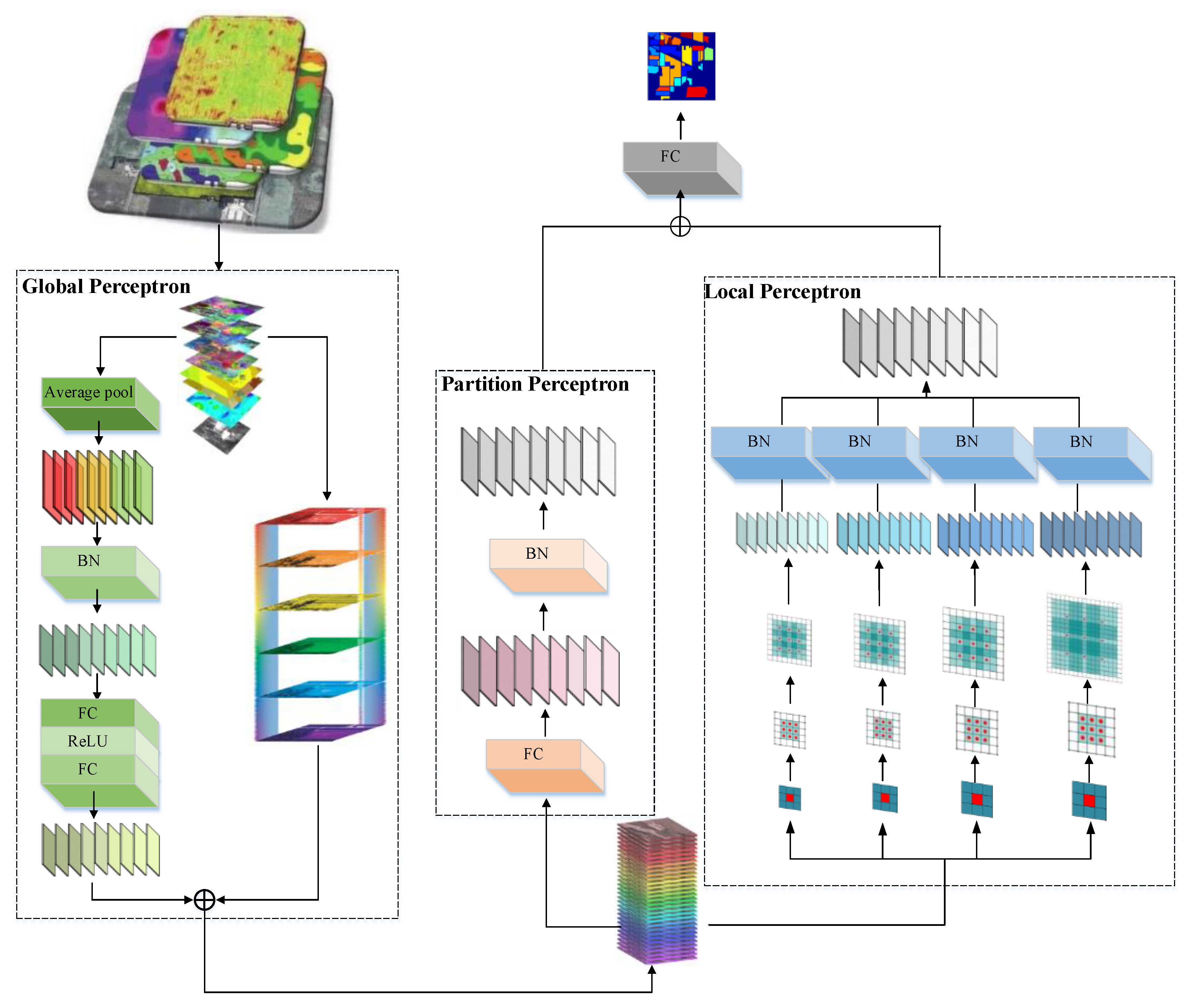
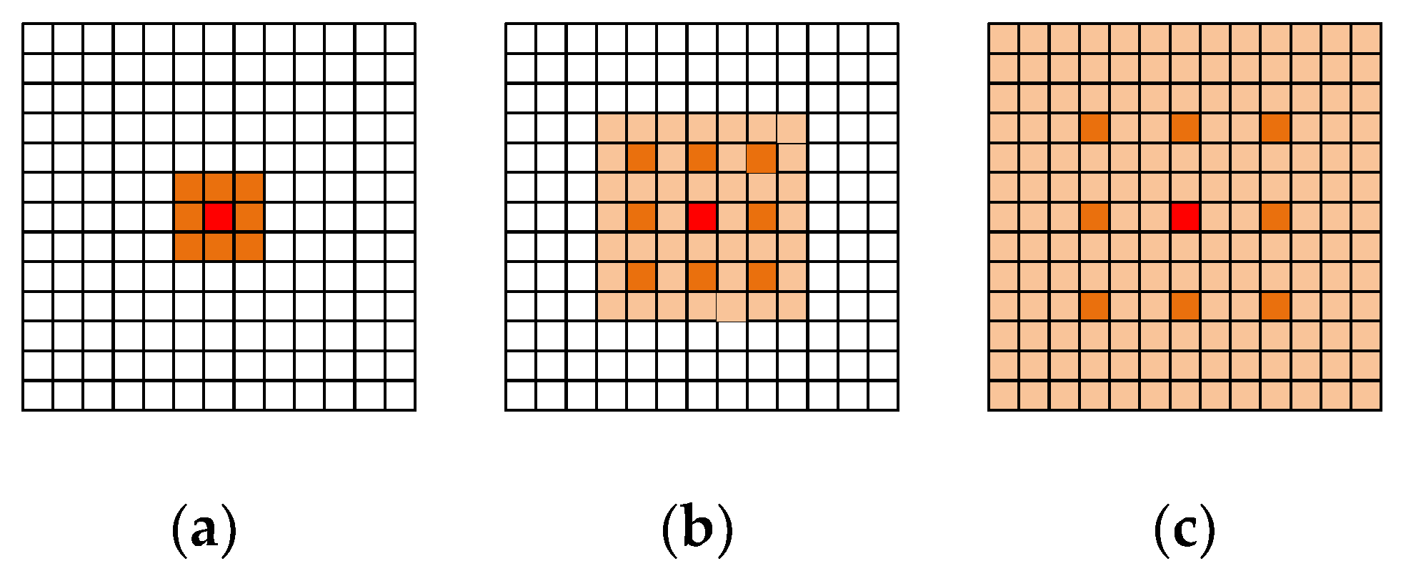
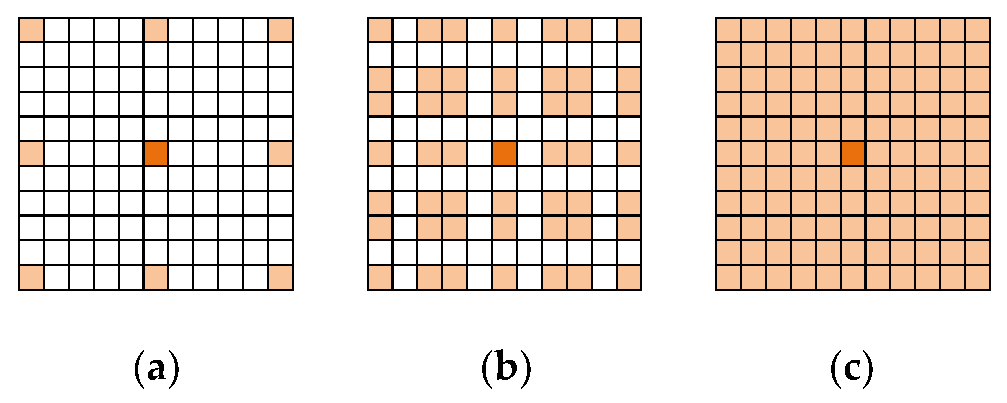
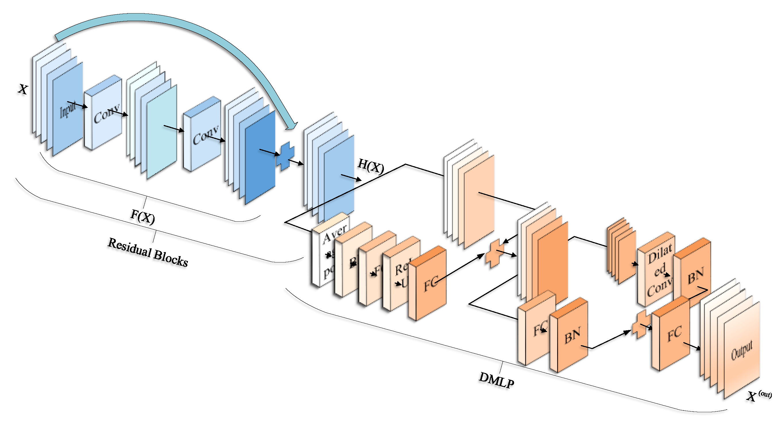
  • MLP, as a less constrained network, can eliminate the negative effects of translation invariance and local connectivity. Therefore, this paper modified MLP combined with dilated convolution to fully obtain spectral–spatial features of each sample and improve HSI remote sensing scene classification performance, called DMLP. The dilated convolutional layer replaced the ordinary convolution of MLP, which can enlarge the receptive field without losing resolution and keep the relative spatial position of pixels unchanged.
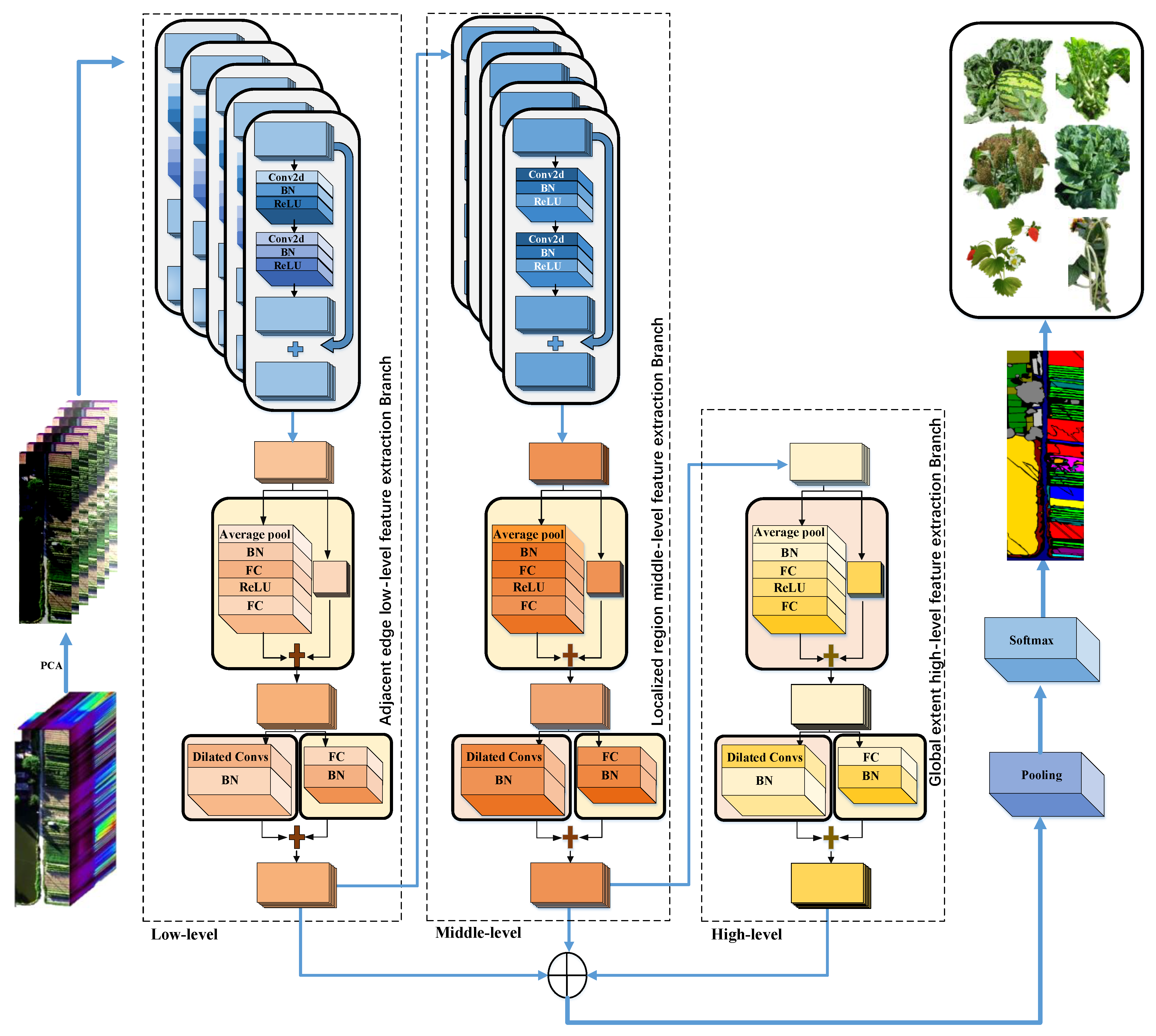
  • This paper composes multi-branch residual blocks and DMLP to form a multi-level feature fusion network, called DMLPFFN. Firstly, the residual structure can retain the original characteristics of the HSI data, and avoid the problems of gradient explosion and gradient disappearance in the training process. In addition, DMLP can improve the feature extraction capability of the residual blocks and strengthen the model with essential features while retaining the original features of the hyperspectral data. In DMLPFFN, three branches of features are fused to obtain a feature map with more comprehensive information, which integrates the spectral information, spatial context information, spatial feature information and spatial location information of HSI to improve classification accuracy.
  • Comprehensive experiments are designed and executed to prove the effectiveness of DMLPFFN by different hyperspectral datasets. DMLPFFN achieved better classification performance and generalization ability for fine crop classification.
The rest of this article is organized as follows. Section 2 describes our proposed classification approach in detail. Section 3 reports the experimental results and evaluates the performance of the proposed method. The application of the model to fine crop classification is given in Section 4. Section 5 analyzes how to choose experimental parameters in DMLPFFN and Section 6 gives the conclusion.

2. The Proposed MLP-Based Methods for HSI Classification

Figure 1 shows the overall framework of our proposed DMLPFFN for HSI classification, which takes the WHU-Hi-LongKou dataset as an example. First, principal component analysis (PCA) is applied to the original HSI to reduce its spectral dimension to weaken the Hughes phenomenon and decrease the burden of model training. At first, the DMLP is structured by altering the normal convolution with the dilated convolution in the local perceptron module of the MLP, thus facilitating the aggregation of contextual information without conceiving a loss of feature map resolution so as to upgrade the classification performance of hyperspectral features.
In addition, DMLPFFN combines residual blocks of different sizes and DMLP to obtain three feature extraction branches, which can fuse three different levels of features and achieve feature maps with more comprehensive information. In the DMLPFFN, multiscale features of the HSI are extracted by a hierarchical different-scale feature extraction branches at different stages of the network. The low-level feature extraction branch of DMLPFFN extracts texture feature information such as color and the edge of ground objects, the middle-level branch extracts regional information and high level is used to extract semantic information with DMLP. The feature fusion is then performed by element summation of the results of the three branches, which can achieve feature maps with more comprehensive information. Then, the global average pooling transforms the feature maps into feature vectors and subsequently obtains the classification results by the softmax function.

2.1. The Proposed Dilation-Based MLP (DMLP) for HSI Classification

Figure 2 shows the overall architecture of the proposed DMLP for HSI classification. The network consists of the global perceptron module, the partition perceptron module and the local perceptron module. Since the MLP has a more powerful representation than convolution, we propose DMLP to accurately represent the feature location information, and retain spatial resolution without loss of detail information.

2.1.1. The Global Perceptron Module Block

It is assumed that the HSI dataset is size H × W × n B a n d , where H and W represent spatial height and width, and n B a n d is the number of bands. First, each pixel of the hyperspectral image is processed with a fixed window size y × x , and a single sample with a shape of y × x × n B a n d is generated. The global perceptron uses shared parameters for different partitions, diminishing the parameters taken for computation and increasing the connection and correlation between the partitions. The global perceptron module block consists of two branches. The first branch splits up the input hyperspectral feature image. The hyperspectral feature map changes from ( H 1 , W 1 , C 1 ) to ( h 1 , w 1 , O ) . H 1 , W 1 , C 1 indicate the height, width and number of input channels of the input hyperspectral feature map. h 1 , w 1 , O , respectively, represent the height, width and number of output channels of the split hyperspectral feature image.
In the second branch, the original feature map ( H 1 , W 1 , C 1 ) is average pooled, and the size of the hyperspectral feature map becomes ( h , w ,   O ) as follows:
h 1 = H 1 h   ,   w 1 = W 1 w
where h and   w indicate the height and width of the hyperspectral feature image after average pooling; the second branch uses h and   w to obtain a pixel for each hyperspectral feature image, and then feeds them though batch normalization (BN) and a two-layer MLP. The hyperspectral feature map ( h , w , O ) is sent to a BN layer and two fully connected layers. The Rectified Linear Unit (ReLU) function is introduced between the two fully connected layers to effectively avoid gradient explosion and gradient disappearance. For the fully connected layer, X ( i n ) and X ( o u t ) represent input and output; the kernel W R Q × P is the matrix multiplication (MMUL) defined as follows:
X ( o u t ) = M M U L ( X ( i n ) , W ) = X ( i n ) W T
The hyperspectral vector was transformed into ( 1 , 1 , C 1 ) by the BN layer and two fully connected layers. Then, the hyperspectral feature images were obtained after all branches were added. Next, we directly fed the input hyperspectral feature into partition perceptron and local perceptron without splitting.

2.1.2. The Partition Perceptron Module Block

The partition perceptron module block contains a BN layer and a group convolution. The input of the partition perceptron is ( h , w , O ) . After the BN layer and group convolution processing, ( h , w , O ) becomes the original hyperspectral feature input ( H 1 , W 1 , C 1 ) .   Y ( o u t ) R C 1 × H 1 × W 1 indicates the output hyperspectral feature and can be obtained as follows:
Y ( o u t ) = g ( Y ( i n ) , F , g , p ) ,   F R C 1 / g × K × K
where p   is the number of pixels filled. F R C 1 / g × K × K is the convolution kernel and g indicates the number of convolution groups.

2.1.3. The Local Perceptron Module Block

To enhance the extraction of high-level semantic information from hyperspectral feature maps without multiplying the calculation parameters, the local perceptron module introduces a dilated convolutional layer [25] and BN layer. First, the local perceptron module simultaneously sends the segmented hyperspectral feature image ( h , w , O ) to the dilated convolution layer. Then, the feature graph is fed into the BN layer. Finally, the output of all convolution branches and the partition perceptron is summarized as the final result.
Specifically, the dilated convolutional layer uses the odd–even mixed dilation rates to stack in each chain, resulting in the expanded receptive field. In addition, under the premise of the same receptive field, the dilated convolution with increased dilation rate consumes fewer training parameters than the extended receptive field with a large convolution kernel. The calculation of the size of the dilated convolution kernel and the receptive field is shown in Formulas (4) and (5), respectively:
f n = f k + ( f k 1 ) ( D r 1 )
l m = l m 1 + [ ( f n 1 ) i = 1 m 1   S i ]
f k represents the size of the original convolution kernel; f n represents the size of the dilated convolution kernel; D r represents expansion rate; l m 1   represents the receptive field size of the ( m 1 ) layer; l m is the size of the m layer receptive field after the convolution; S i represents the step size of layer i .
The equivalently fully connected layers (FC) kernel of a Dilated Conv kernel is the result of convolution on an identity matrix with proper reshaping. Formula (6) shows exactly how to build W ( F , p ) from F and p .
W ( F , p ) = D i l a t e d C O N V ( Y , F , p ) , ( C h w , O h w ) T
The convolution after multiple superimpositions of the expansion may lead to a grid effect, as shown in Figure 3. This will cause some dilution between pixels, which causes some pixels to be omitted, resulting in the loss of local information and undermining the continuity of information.
Considering the grid effect, the design of the expansion rate in the DMLP model proposed in this paper follows Equation (7).
M i = max [ M i + 1 2 r i , M i + 1 2 ( M i + 1 r i ) , r i ]
where r i is the expansion rate of layer i and M i is the maximum expansion rate of layer i . Mixed dilated convolution requires that the expansion rate of superposition convolution cannot have a common divisor greater than 1. As shown in Figure 4, in this paper, the method of mixed parity expansion rate is used to expand the convolution kernel, and the expansion rate is set to the cyclic structure [1,2,5], which can cover every pixel on the image to avoid information loss.

2.2. The Proposed DMLPFFN Model for HSI Classification

Features at various levels contain diverse information distribution. The lower-level features contain rich spatial structure information, but their high resolution leads to weak global background information. The higher-level features have rich semantic information and can effectively classify hyperspectral images, but their poor resolution lacks spatial details for the hyperspectral images [26]. For this reason, the fusion of these different levels of feature information can significantly strengthen the classification accuracy of hyperspectral images. The paper proposes DMLPFFN, which can extract sufficiently different level features by fusing three feature extraction branches, as shown in Figure 1.

2.2.1. Fusion of Multi-Branch Features

As the layer of the network deepens, the feature information obtained during the feature extraction of the convolutional network will be different for each branch. Figure 5 shows the structure of residual blocks with DMLP, called the adjacent edge low-level feature extraction branch (the left branch in Figure 1), which is used to to obtain texture characteristic information such as the color and border of the ground target.
The residual block is introduced to connect each layer to other layers in a feed-forward fashion. According to the structure of the residual unit, X represents input, H ( x ) represents output and F ( x ) represents a residual unit. The residual unit carries out identity mapping of input at each layer from top to bottom, and the features of input are learned to form the residual function [27]. Then, the output of the residual unit becomes H ( x ) = F ( x ) + x . Therefore, the residual function can deal with more advanced abstract features when the number of network layers increases, and is easier to optimize. The calculation process of the residual element is shown in Formula (8):
F ( x ) = W 2 σ ( W 1 x )
where σ stands for nonlinear function ReLU and W 1 and W 2 are the weights of layer 1 and layer 2, respectively. Then, the residual unit goes through a shortcut and a second ReLU layer to obtain the output H ( x ) :
H ( x ) = F ( x , { W i } ) + x
When the dimension size of the input and the output needs to be changed, a linear transformation can be performed in a shortcut operation, as shown in Formula (10):
H ( x ) = F ( x , { W i } ) + W s x
By stacking multiple residual blocks, the extracted features become increasingly discriminative. Then, we connect the output of the residual block to the input of the DMLP. H ( x ) ( i n ) and X ( o u t ) represent input and output and the kernel W R Q × P is the matrix multiplication (MMUL) defined as follows:
X ( o u t ) = M M U L ( H ( x ) ( i n ) , W )
This structure extracts more abstract features and discards redundant information through the DMLP module. The introduction of DMLP brings fewer parameters and higher operational efficiency and speed compared to simply increasing the depth of the residual network. In addition, it improves the global feature learning capability and the nonlinearity for the model, resulting in a better abstract representation of the model.
The middle-level branch focuses on extracting regional information with a similar structure of a low-level feature extraction branch. Middle-level features focus more on regional features than lower-level features, which is of great significance to the extraction of spatial structure features of HSIs. The high-level branch uses DMLP to extract global features, which keeps the relative spatial position of pixels unchanged and obtains the context information of the HSIs.
In detail, assume that O 1 , O 2 and O 3 refer to the outputs of the low-, middle- and high-level feature extraction branch, which has 16, 32 and 64 feature maps, respectively. Then, the resultant maps of the three branches are convolved with 64 kernels of size 1 × 1 in this paper. By means of such convolution operations, the number of feature maps of O 1 , O 2 and O 3 all become 64. Eventually, feature fusion can be conveniently performed by element summation as follows:
T = i = 1 3 & j = 1 3 P o o l i n g ( f i ( O j ) )
where T represents the fused features, f 1 , f 2 and f 3 are the dimension matching function and Pooling is the global averaging function.
The proposed DMLPFFN model enhances the resemblance between the same hyperspectral feature objects and the variability between the exotic objects to accomplish high-precision classification of crop species.

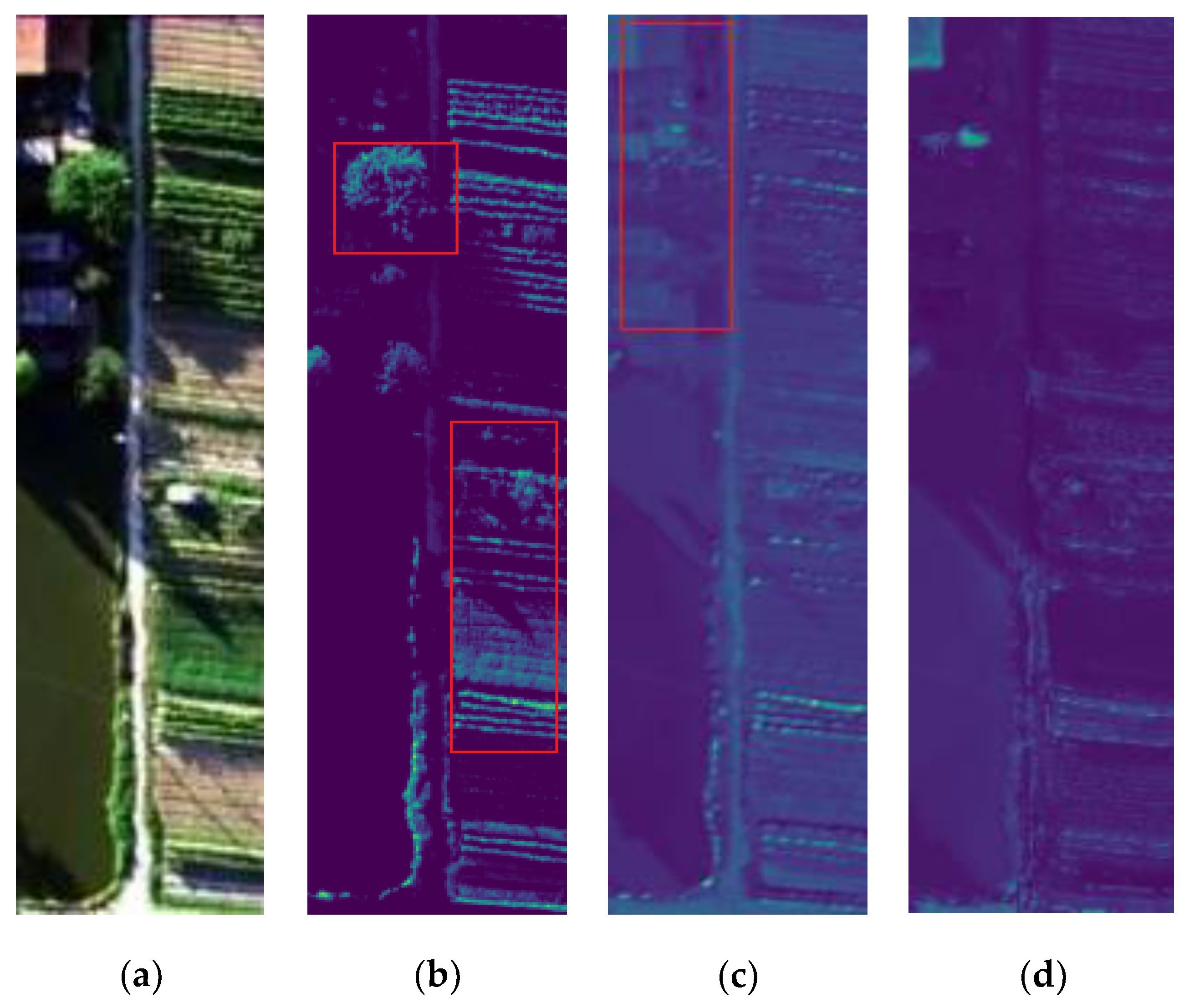
2.2.2. Feature Output Visualization and Analysis

In order to better analyze the characteristics of feature extraction of DMLPFFN, this paper visualizes the feature maps of different branches, as shown in Figure 6.
Figure 6b–d shows the feature output plots for the adjacent edge low-level feature extraction branch, localized region middle-level feature extraction branch and global extent high-level feature extraction branch, respectively. As shown in the red frame in Figure 6b, detailed features as edges and textures of trees and farmland are highlighted. Figure 6c shows the crop regionality is enhanced and this branch extracts the regional information of the image. In Figure 6d, the global and abstract nature of the extracted features of the image is made more apparent. In summary, Figure 6 shows the difference of the extracted features in each branch and it is necessary to fuse multi-branch features to fully dig spatial and spectral features of HSI.

3. Experimental Results

3.1. Public HSI Dataset Description

In order to verify the effectiveness of the proposed method, classification experiments were performed on two standard hyperspectral datasets (Salinas and KSC) [28,29]. The details of each dataset are as follows. The Salinas dataset was acquired by an Airborne Visible-Infrared Imaging Spectrometer (AVIRIS) sensor at the Salinas Valley in California and consists of 512 × 217 pixels and 224 spectral reflectance bands. The number of bands was reduced to 204 by removing the bands covering the water-absorbing area (108–112, 154–167, 224). Ground Truth contains 16 types of land cover. The KSC dataset was picked up by AVIRIS sensors flying over the Kennedy Space in Florida. The number of spectral bands is 176, and the size is 512 × 614 pixels with 13 categories.
Table 1 and Table 2 report the detailed number of pixels available in each class for the two datasets, respectively, and show the false-color composite image and ground truth map.

3.2. Experimental Parameter Setting

All experiments were performed on Intel(R) Xeon(R) 4208 CPU @ 2.10GHz processor and Nvidia GeForce RTX 2080Ti graphics card. In order to reduce experimental errors, the model randomly selected a limited number of samples from the training set for training. The epoch was set to 200. All experimental results were averaged from 10 experiments. Overall accuracy (OA), average accuracy (AA) and Kappa coefficient (K) were used as evaluation indexes to measure the performance of each method. The initial learning rate of this method was 0.1 and was then divided by 10 when the error plateaued. The networks are trained for 2 × 10 4 iterations and the training minibatch has a size of 100. We use a weight decay of 0.0001 and a momentum of 0.9.

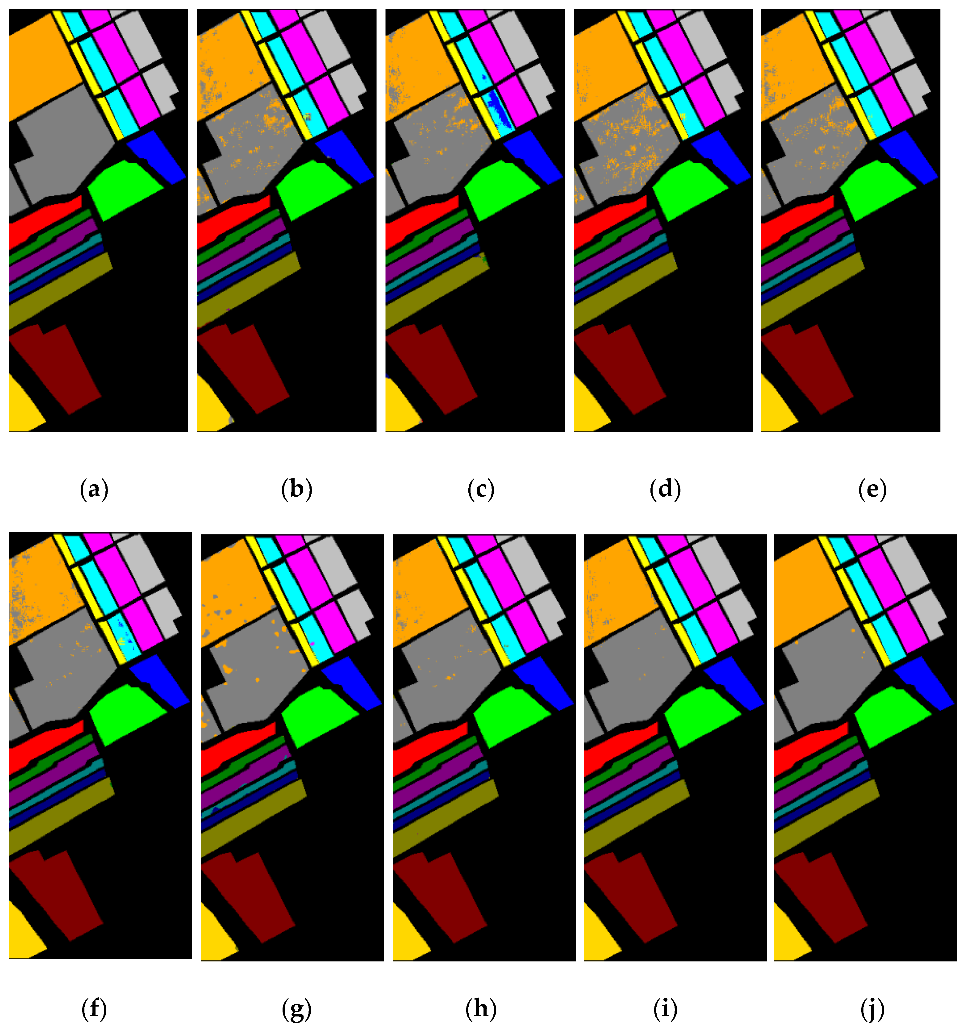
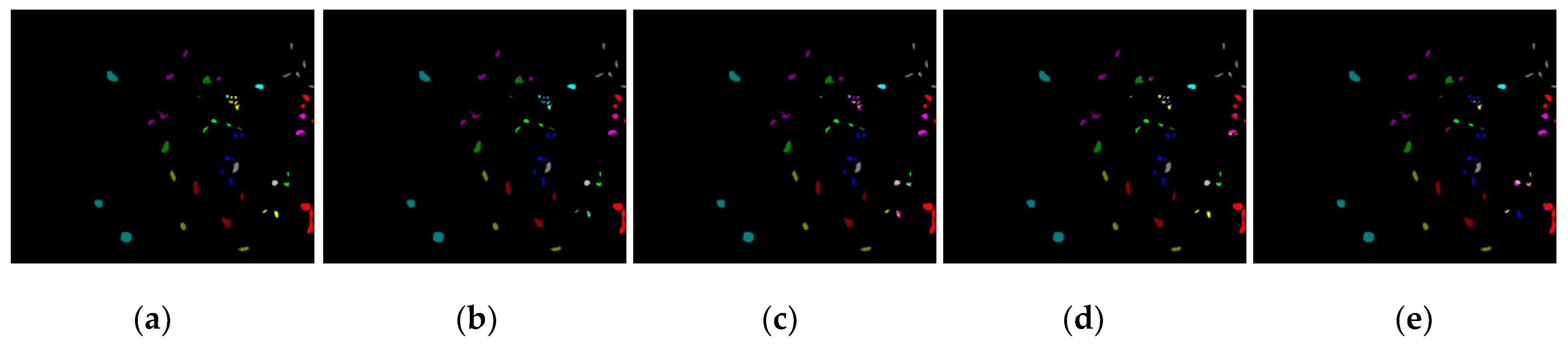
3.3. Comparison of the Proposed Methods with the State-of-the-Art Methods

The experiment mainly compares the proposed algorithm DMLP and DMLPFFN with the Radial Basis Function (RBF) Support Vector Machine algorithm (RBF-SVM) [30] and Extended Morphological Profile (EMP) Support Vector Machine Methods (EMP-SVM) [31], Convolutional Neural Network (CNN) [32], Residual Network (ResNet) [33], MLP-Mixer, RepMLP [34] and Deep Feature Fusion Network (DFFN) [35] classification performance for the hyperspectral dataset. Ten percent of the total sample number was used as the training sample number for hyperspectral classification as shown in Table 3, Table 4 and Table 5. Compared with other methods, the DMLPFFN method proposed in this paper has the highest classification accuracy for two datasets.
Taking Salinas dataset as an example, compared with RBF-SVM, OA, AA and Kappa coefficients of DMLPFFN increased by 13.01%, 11.47% and 10.72%, and improved by 2.07%, 2.67% and 2.31% compared with DFFN, respectively. Taking the KSC dataset as an example, OA reached 98.49%, compared with RBF-SVM, EMP-SVM, CNN, ResNet, MLP-Mixer, RepMLP and DFFN, increased by 16.84%, 14.52%, 12.45%, 7.74%, 5.08%, 3.56%, 2.67% and 1.73% respectively. AA reached 97.65%, compared with DFFN, RepMLP, MLP-Mixer, ResNet, CNN, EMP-SVM and RBF-SVM, increased by 2.41%, 3.44%, 4.47%, 5.30%, 8.54%, 11.60%, 15.08% and 17.74%. All the experimental results show that the proposed DMLPFFN is superior to other methods.
In order to fully analyze the effect of the water absorption band on the experimental results, we downloaded the Salinas dataset with the water absorption band from the official website and conducted experimental analysis on it. As shown in Table 4, compared with RBF-SVM, OA, AA and Kappa coefficients of DMLPFFN increased by 16.89%, 15.10% and 14.61%, and improved by 3.80%, 3.15%, and 3.81% compared with DFFN, respectively. All the experimental results show that the proposed DMLPFFN is superior to other methods on the Salinas dataset with the water absorption bands.
Besides the quantitative classification results reported, we simultaneously visualized the classification maps of different methods discussed above, as shown in Figure 7 and Figure 8.
Obviously, it can be seen that RBF-SVM results have the most misclassified pixels in all classification maps, with many pretzel noises throughout, and each part is unavoidable for the classification confusion. Taking the dataset of Salinas as an example, in Figure 7b–d, a large amount of noise is generated in the upper left corner. Part of the area Vinyard untrained was misclassified as grapes_untrained. The classification confusion of Grapes_untrained, Grapes_untrained and Fallow_rough_pow in the middle part is serious. Compared with SVM, CNN and ResNet classification methods, the classification effect of MLP-Mixer, RepMLP and DFFN is improved, but there are still some misclassification phenomena. In addition, Figure 7i,j are the classification renderings of our algorithm; an obvious observation is that the classification map of the proposed method is the closest to the reference ground truth, which produces less internal noise and a cleaner boundary. Experiments show that the proposed method can effectively extract more refined features from two kinds of datasets, and cross-dimensional information interaction focuses on more important features, thus improving the classification accuracy.

4. Application in Fine Classification of Crops

In order to verify the classification performance and generalization ability of the DMLP and DMLPFFN, the WHU-Hi-LongKou and WHU-Hi-HanChuan hyperspectral datasets were selected in this paper for fine crop classification [36,37].
The WHU-Hi-LongKou dataset is located in a simple agricultural area and was captured by an 8 mm focal length steeple-wall Headwall Nano-HyperSpec sensor equipped with a receiver Matrix 600 Pro UAV platform with six kinds of crops. The image size was 550 × 400 pixels, with 270 bands between 400 and 1000 nm. The WHU-Hi-HanChuan dataset was collected in HanChuan, Hubei Province, using a 17 mm focal length Headwall Nano-HyperSpec sensor installed on the Leica Aibot X6 UAV V1 platform. The trial area has seven kinds crops and size 1217 × 303 pixels with 274 bands ranging from 400 to 1000 nm. Table 6 and Table 7 report the detailed number of pixels available in each class for the two datasets, respectively, and show the false-color composite image and Ground Truth map.
In LongKou dataset, soybean occupies a prominent position, and its plot is continuous and extensive. Sesame and cotton are interlaced around the corn planting field. As shown in Table 8, the OA of DMLPFFN obtained 99.16%. Among all classification groups, the classification method DMLPFFN proposed in this paper has the highest OA, AA and Kappa coefficients, reaching 99.16%, 98.59% and 96.88, respectively. Compared with RBF-SVM, EMP-SVM, CNN, ResNet, MLP-Mixer, RepMLP, DFFN and DMLP, OA increased by 10.00%, 6.95%, 4.38%, 3.53%, 2.84%, 1.58%, 1.19% and 0.91%, respectively.
As shown in Table 9, in the HanChuan dataset, there are only a small number of soybean samples with 1335 pixels, thus affecting the classification effect of various algorithms. For soybean with poor classification performance in other algorithms, the accuracy of the two algorithms proposed in this paper can reach 93.37% and 94.16%, indicating that DMLP and DMLPFFN algorithms are suitable for separating similar ground objects. The methods proposed in this paper effectively solve the problem of spectral variation and heterogeneity within the same object.
Experimental results corresponding to different classification algorithms are shown in Figure 9 and Figure 10 for HanChuan and LongKou datasets, respectively. As shown in Figure 9, it can be seen that there are still a large number of “salt and pepper” noises in RBF-SVM and EMP-SVM. The classification results of CNN and ResNet methods showed that the noise was greatly reduced after considering the contextual information. The classification results of ResNet, MLP-Mixer, RepMLP and DFFN methods showed that a large part of the samples of strawberry, cowpea, soybean and water oat were incorrectly classified into other categories in the middle region of the dataset. This is due to the fact that sowing at the edge of the field is even less compact than sowing in the center. The network misclassified crops as other categories at the margins of some plots owing to the sparse distribution of plants causing leakage of bare land area. Moreover, soybeans and cowpeas are crops of the same origin and exhibit highly similar spectral properties in a certain wavelength range, carrying a negative burden on the classification. Nevertheless, in our approaches, there is barely any misclassification of dense plants in the marginal areas and in the center of the plots, indicating that our method effectively discriminates between confusing crop classes due to spectral variation.
The color and edge features extracted from the low-level branch enable one to distinguish more conveniently between different types of crops and amplify the differences between different crops, whereas the regional features extracted in the middle-level branch lead to more apparent boundaries between crops in different places and perform better identification of crop areas and non-crop areas. The global features extracted at the high level minimize the clutter between sophisticated backdrops and crops to a certain extent and provide a better assessment of the overall crop area. Multi-level feature fusion can sufficiently extract and leverage the feature information of crops and fine classifications of them. Consequently, DMLPFFN is considered suitable for fine crop classification.

5. Discussion

In order to find the optimal network structure, it is necessary to experiment with different parameters, which play a crucial role in the size of the model and the complexity of the proposed DMLPFFN. In this paper, the optimal parameter combination is determined by analyzing the influence of parameters on the accuracy of classification results, including the number of PCAs, the expansion rate of dilated convolution, the percentage of training samples and the number of branches in the feature fusion strategy.

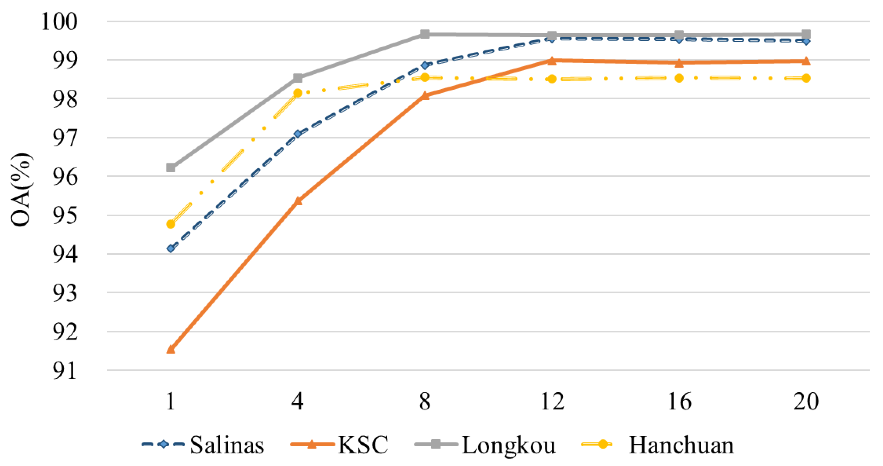
5.1. The Number of Principal Components

The first parameter is the number of principal components selected for PCA on HSI, which is used to extract the main spectral components to improve the algorithm’s efficiency and reduce noise interference. In the case of principal component number, the control variable method is used for all datasets in the experiment. That is to say, the value of training sample number, expansion rate and deep feature fusion strategy is fixed. As shown in Figure 11, OA increased and then tended to be stable with the increase of the principal component number for the four HSI datasets. Most of the information in the hyperspectral image exists in the first few principal components. However, it was concluded that using many principal components did not further improve performance.

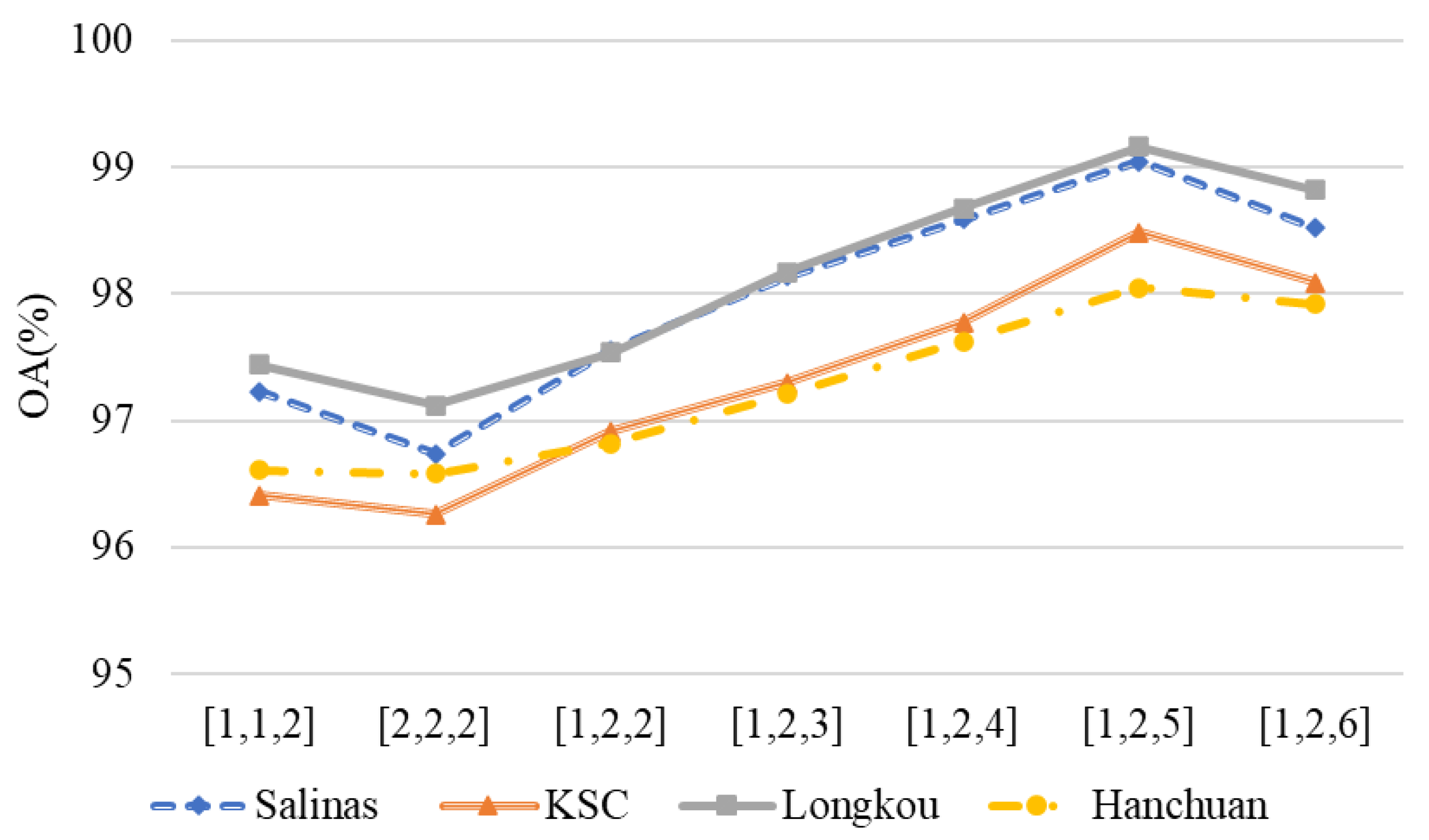
5.2. The Expansion Rate of Dilated Convolution

The second parameter is the distribution of the expansion rate. In this experiment, seven circulation structures with expansion rate distributions of [1,1,2], [2,2,2], [1,2,2], [1,2,3], [1,2,4], [1,2,5] and [1,2,6] are selected for comparative analysis, as shown in Figure 12.
By comparing the experimental results, it can be found that the classification accuracy of the expansion rate distributions of [1,1,2] is lower than that of the expansion rate distributions of [1,2,2]. The receptive field size of [1,1,2] is 9 × 9 . In [2,2,2], although the range of the receptive field increases to 13×13, the classification accuracy is lower than the average overall accuracy of the expansion rate distributions of [1,1,2]. This is because the superposition of three dilated convolutions will result in more feature information being omitted.
The latter five experiments used the combination of two dilated convolution layers and one ordinary convolution layer, and the receptive fields were 11 × 11 , 13 × 13 , 15 × 15 , 17 × 17 and 19 × 19 . Nonetheless, [1,2,5] has the largest range of receptive fields; with the increase of expansion rate, the data of input sampling become more and more sparse, resulting in local information loss and damage to information continuity. According to the experimental results in Figure 12, when the expansion rate distribution is [1,2,5], the four HSI datasets can obtain the optimal classification results.

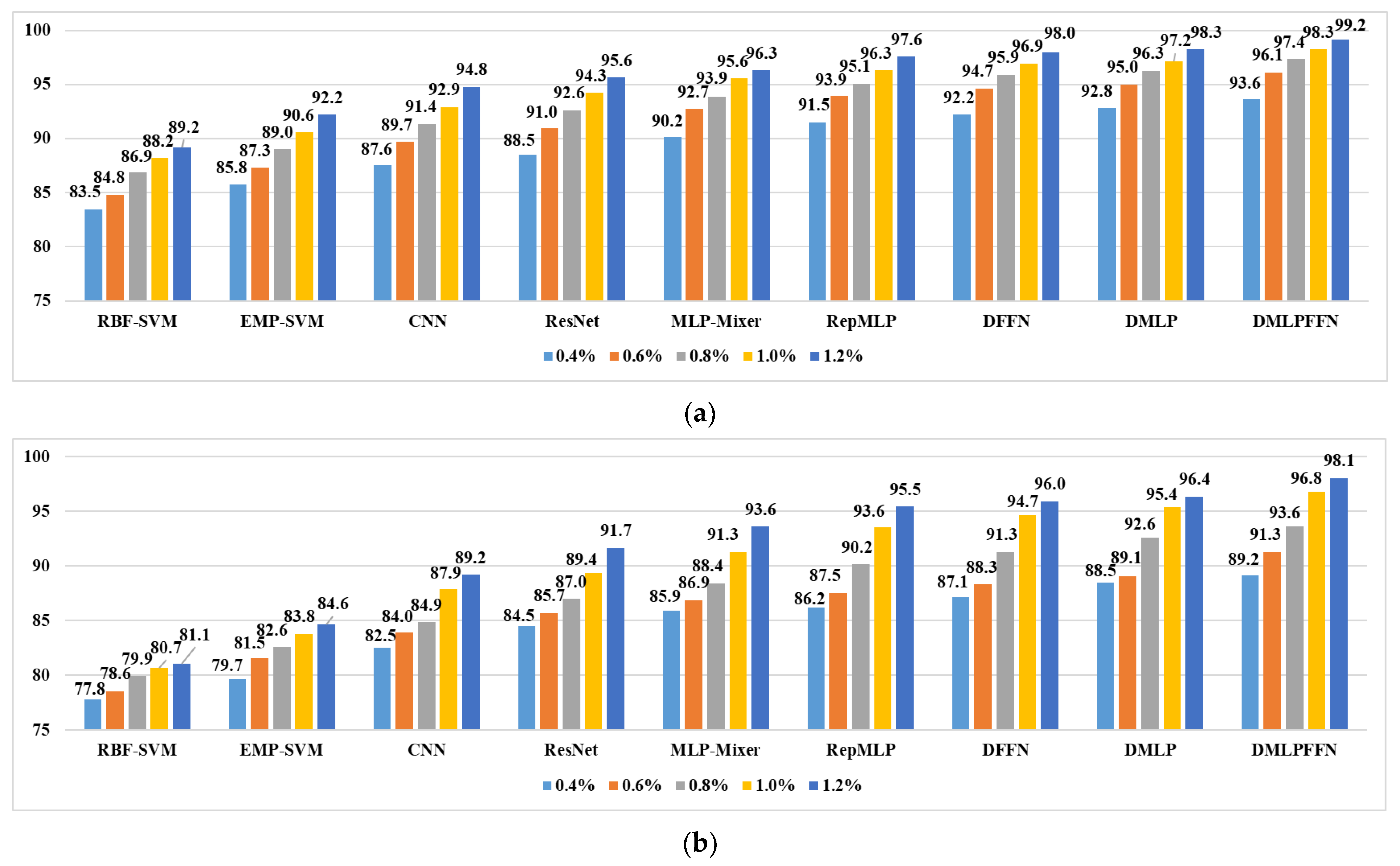
5.3. The Percentage of Training Samples

The third parameter is the proportion of training samples to the total number of samples. We carried out experiments on the practical crop hyperspectral datasets LongKou and HanChuan, as shown in Figure 13. 0.4%, 0.6%, 0.8%, 1.0% and 1.2% of LongKou and HanChuan dataset training samples were selected for experiment, respectively. At the beginning, the classification accuracy increased with training samples. When the training sample of LongKou and HanChuan datasets was 1.2%, the OA value basically reached the highest point and then tended to be flat or even showed a downward trend. When the number of training samples reaches the required level, it can precisely illustrate the distribution of all pixels in the studied area; continuously increasing the number of training samples will not increase the classification accuracy. Therefore, 1.2% is chosen as the percentage of training samples, and the proposed DMLPFFN method always provides better performance than other comparison methods.

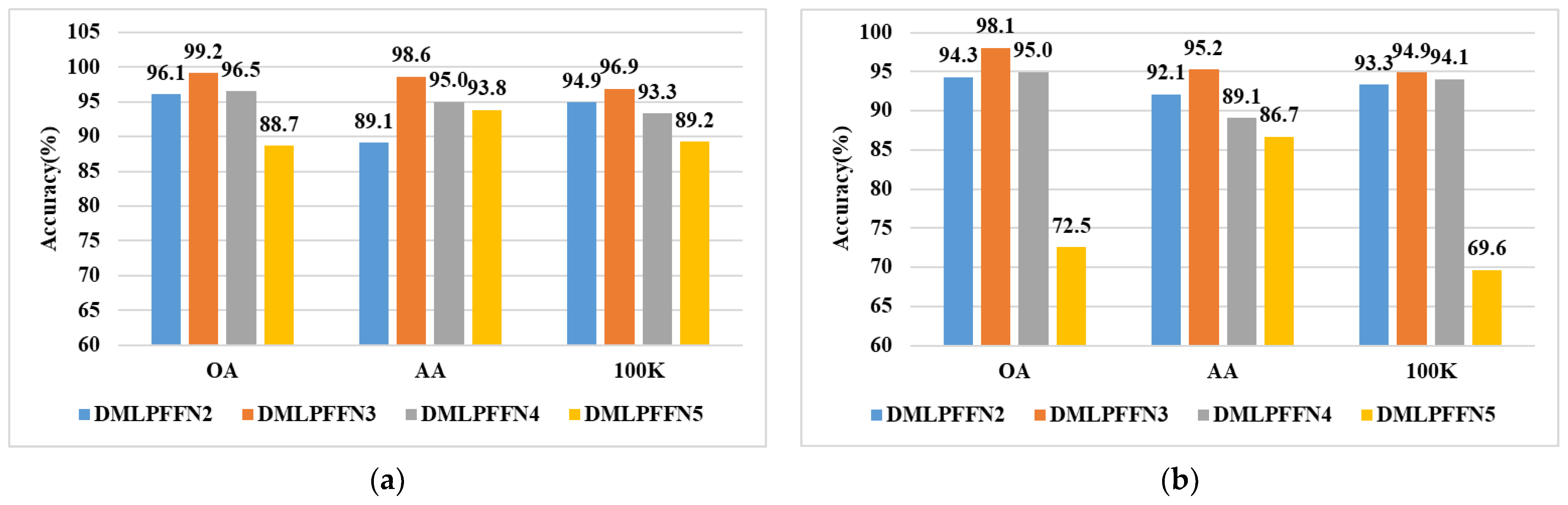
5.4. The Number of Branches in Feature Fusion Strategy

The fourth parameter is the number of branches in feature fusion strategy. This paper analyzes the correlation and complementarity of information in the deep network using multibranch feature fusion. DMLPFFN2, DMLPFFN3, DMLPFFN4 and DMLPFFN5 refer to methods that fuse two, three, four and five hierarchical branches. Among them, DMLPFFN2 represents the fusion of lower-level and higher-level sorts. It can be seen from Figure 14 that in different datasets, DMLPFFN3 obtained precision values that are superior to DMLPFFN2, DMLPFFN4 and DMLPFFN5. In addition, taking the LongKou dataset as an example, compared with the DMLPFFN2, the OA, AA and Kappa values of the DMLPFFN3 fusion strategy increased by 3.05%, 9.5%, and 1.97%, respectively. That is because the features extracted by DMLPFFN2 contain only details and global information, and regional feature information is dropped. To some extent, fusing multiple layers improves classification results. However, DMLPFFN5 has the lowest classification accuracy, which shows that too many fusion layers may bring redundant information and significantly reduce the performance. Specifically, middle-level information overlap can cause accuracy degradation. So the DMLPFFN method proposed in this paper used three branches for feature fusion and the structure is as shown in Figure 1.

5.5. The Number of Classes for HSI Classification

We conducted experiments on the KSC dataset for different numbers of classes. The KSC dataset was picked up by AVIRIS sensors flying over the Kennedy Space in Florida. The number of spectral bands is 176, and the size is 512 × 614 pixels with 13 classes. Table 10 shows the OA, AA and Kappa values of the DMLPFFN method when the number of classes is 10, 11, 12 and 13. The results show that the accuracy of the result decreases when the number of classes reduces. The highest precision is achieved when the number of classes is 13, which is the original number of classes. This shows that if the number of classes in the experimental dataset is not utilized sufficiently, it will lead to a decrease in the accuracy of the experimental results.

5.6. Time Consumption and Computational Complexity

In order to comprehensively analyze the methods proposed in this paper and current research methods, this paper analyzes the average training time, average test time and total parameters of different methods. Table 11 reports the time consumption and computational complexity of different methods.
In terms of running time, taking the HanChuan dataset as an example, although DMLP has a larger receptive field to extract more delicate features and consumes more training time than RepMLP, the total parameters are reduced by 22.98%. Moreover, compared with ResNet and the MLP-Mixer, the training times of DMLP are reduced by 59.65% and 15.15%, and DMLP has better classification accuracy. The results show that, compared with ResNet, DMLP and DMLPFFN have fewer parameters on all datasets. Compared with CNN and the MLP-Mixer, the proposed method has a few more parameters because of its greater depth and width, but the accuracy of the proposed method is the highest. Moreover, compared with DFFN, DMLPFFN has a shorter training time on four datasets because DMLPFFN improves the training performance of the model by combining the fusion strategy with MLP. Taking the LongKou dataset as an example, DMLPFFN training time and test time are reduced by 25.20% and 25.28%, respectively, compared with DFFN. In addition, DMLPFFN has the lowest training time and test time next to CNN among all deep learning methods and achieves better OA than other classification algorithms.

6. Conclusions

In this paper, two classification frameworks based on MLP are proposed: DMLP and DMLPFFN. Firstly, in order to expand the perceptual field and aggregate multi-branch contextual information and avoid losing the feature map resolution, we introduced a dilated convolution layer instead of ordinary convolution. Secondly, for the purpose of fully utilizing the features of HSI to improve the classification efficiency, we use fusing residual blocks and the DMLP mechanism to extract deeper features and obtain the state-of-the-art performance. Finally, we designed comprehensive experiments and executed them to prove the effectiveness of DMLPFFN by different hyperspectral datasets and to prove that it has better classification performance and generalization ability for agricultural classification.
The proposed DMLP and DMLPFFN were tested on two public datasets (Salinas and KSC) and two real HSI datasets (LongKou and HanChuan). Compared with the classical methods (RBF-SVM and EMP-SVM) and deep learning-based methods (CNN, ResNet, MLP-Mixer, RepMLP and DFFN), the experiments show that the proposed DMLP algorithm and DMLPFFN algorithm are meaningful and can obtain better classification results. We also validate the classification performance and generalization ability of DMLPFFN in fine crop classification, which contributes to promoting the specific application of hyperspectral remote sensing technology in agricultural development.
However, in the task of hyperspectral image classification, the available marker samples are usually very limited. When analyzing the classification effect of the number of training samples, take the KSC dataset as an example; the DMLPFFN proposed in this paper reveals that an effectiveness of 10% of the sample size is superior to the others. As a future step, we are conducting further experiments to probe the prevalence suitability of DMLPFFN in small sample cases.

Author Contributions

Conceptualization, A.W., H.Z. and H.W.; methodology, software, validation, H.Z.; writing—review and editing, H.W. and A.W.; supervision, Y.I. All authors have read and agreed to the published version of the manuscript.

Funding

This work was funded by the National Natural Science Foundation of China under Grant NSFC-61671190.

Data Availability Statement

Acknowledgments

We thank for Kaiyuan Jiang for his valuable comments and discussion. Iwahori’s research is supported by JSPS Grant-in-Aid for Scientific Research (C) (20K11873) and Chubu University Grant.

Conflicts of Interest

The authors declare no conflict of interest.

References

  1. Czaja, W.; Kavalerov, I.; Li, W. Exploring the High Dimensional Geometry of HSI Features. In Proceedings of the 2021 11th Work-Shop on Hyperspectral Imaging and Signal Processing: Evolution in Remote Sensing (WHISPERS), Amsterdam, The Netherlands, 24–26 March 2021; pp. 1–5. [Google Scholar]
  2. Zhang, Y.; Wang, D.; Zhou, Q. Advances in crop fine classification based on Hyperspectral Remote Sensing. In Proceedings of the 2019 8th International Conference on Agro-Geoinformatics, Istanbul, Turkey, 16–19 July 2019; pp. 1–6. [Google Scholar]
  3. Kim, Y.; Kim, Y. Hyperspectral Image Classification Based on Spectral Mixture Analysis for Crop Type Determination. In Proceedings of the IGARSS 2018—2018 IEEE International Geoscience and Remote Sensing Symposium, Valencia, Spain, 23–27 July 2018; pp. 5304–5307. [Google Scholar]
  4. Spiller, D.; Ansalone, L.; Carotenuto, F.; Mathieu, P.P. Crop Type Mapping Using Prisma Hyperspectral Images and One-Dimensional Convolutional Neural Network. In Proceedings of the 2021 IEEE International Geoscience and Remote Sensing Symposium IGARSS, Brussels, Belgium, 11–16 July 2021; pp. 8166–8169. [Google Scholar]
  5. Pignatti, S.; Casa, R.; Harfouche, A.; Huang, W.; Palombo, A.; Pascucci, S. Maize Crop and Weeds Species Detection by Using Uav Vnir Hyperpectral Data. In Proceedings of the IGARSS 2019—2019 IEEE International Geoscience and Remote Sensing Symposium, Yokohama, Japan, 28 July–2 August 2019; pp. 7235–7238. [Google Scholar]
  6. Kefauver, S.C.; Romero, A.G.; Buchaillot, M.L.; Vergara-Díaz, O.; Fernandez-Gallego, J.A.; El-Haddad, G.; Akl, A.; Araus, J.L. Open-Source Software for Crop Physiological Assessments Using High Resolution RGB Images. In Proceedings of the IGARSS 2020—2020 IEEE International Geoscience and Remote Sensing Symposium, Waikoloa, HI, USA, 26 September–2 October 2020; pp. 4359–4362. [Google Scholar]
  7. Liu, C.; Li, M.; Liu, Y.; Chen, J.; Shen, C. Application of Adaboost based ensemble SVM on IKONOS image Classification. In Proceedings of the 2010 18th International Conference on Geoinformatics, Beijing, China, 18–20 June 2010; pp. 1–5. [Google Scholar]
  8. Cuozzo, G.; D’Elia, C.; Puzzolo, V. A method based on tree-structured Markov random field for forest area classification. In Proceedings of the IGARSS 2004. 2004 IEEE International Geoscience and Remote Sensing Symposium, Anchorage, AK, USA, 20–24 September 2004; Volume 4, pp. 2352–2354. [Google Scholar]
  9. Li, Z.; Li, X.; Chen, E.; Li, S. A method integrating GF-1 multi-spectral and modis multitemporal NDVI data for forest land cover classification. In Proceedings of the 2016 IEEE International Geoscience and Remote Sensing Symposium (IGARSS), Beijing, China, 10–15 July 2016; pp. 3742–3745. [Google Scholar]
  10. Delalieux, S.; Somers, B.; Haest, B.; Spanhove, T.; Borre, J.V.; Mücher, C.A. Heathland conservation status mapping through integration of hyperspectral mixture analysis and decision tree classifiers. Remote Sens. Environ. 2012, 126, 222–231. [Google Scholar] [CrossRef]
  11. Chen, Y.; Lin, Z.; Zhao, X.; Wang, G.; Gu, Y. Deep Learning-Based Classification of Hyperspectral Data. IEEE J. Sel. Top. Appl. Earth Obs. Remote Sens. 2014, 7, 2094–2107. [Google Scholar] [CrossRef]
  12. Tao, C.; Pan, H.; Li, Y.; Zou, Z. Unsupervised Spectral–Spatial Feature Learning with Stacked Sparse Autoencoder for Hyperspectral Imagery Classification. IEEE Geosci. Remote Sens. Lett. 2015, 12, 2438–2442. [Google Scholar]
  13. Sun, Q.; Liu, X.; Fu, M. Classification of hyperspectral image based on principal component analysis and deep learning. In Proceedings of the 2017 7th IEEE International Conference on Electronics Information and Emergency Communication (ICEIEC), Shenzhen, China, 21–23 July 2017; pp. 356–359. [Google Scholar]
  14. Chen, Y.; Jiang, H.; Li, C.; Jia, X.; Ghamisi, P. Deep Feature Extraction and Classification of Hyperspectral Images Based on Convolutional Neural Networks. IEEE Trans. Geosci. Remote Sens. 2016, 54, 6232–6251. [Google Scholar] [CrossRef] [Green Version]
  15. Zhang, B.; Qing, C.; Xu, X.; Ren, J. Spatial Residual Blocks Combined Parallel Network for Hyperspectral Image Classification. IEEE Access 2020, 8, 74513–74524. [Google Scholar] [CrossRef]
  16. Kanthi, M.; Sarma, T.H.; Bindu, C.S. A 3d-Deep CNN Based Feature Extraction and Hyperspectral Image Classification. In Proceedings of the 2020 IEEE India Geoscience and Remote Sensing Symposium (InGARSS), Virtual, 1–4 December 2020; pp. 229–232. [Google Scholar]
  17. Zhang, H.; Yu, H.; Xu, Z.; Zheng, K.; Gao, L. A Novel Classification Framework for Hyperspectral Image Classification Based on Multi-Scale Dense Network. In Proceedings of the 2021 IEEE International Geoscience and Remote Sensing Symposium IGARSS, Brussels, Belgium, 11–16 July 2021; pp. 2238–2241. [Google Scholar]
  18. Zhu, M.; Fan, J.; Yang, Q.; Chen, T. SC-EADNet: A Self-Supervised Contrastive Efficient Asymmetric Dilated Network for Hyperspectral Image Classification. IEEE Trans. Geosci. Remote Sens. 2020, 60, 1–17. [Google Scholar] [CrossRef]
  19. Tolstikhin, I.O.; Houlsby, N.; Kolesnikov, A.; Beyer, L.; Zhai, X.; Unterthiner, T.; Yung, J.; Steiner, A.; Keysers, D.; Uszkoreit, J.; et al. Mlp-mixer: An all-mlp architecture for vision. arXiv 2021, arXiv:2105.01601. [Google Scholar]
  20. Yu, T.; Li, X.; Cai, Y.; Sun, M.; Li, P. S2-MLP: Spatial-Shift MLP Architecture for Vision. In Proceedings of the 2022 IEEE/CVF Winter Conference on Applications of Computer Vision (WACV), Waikoloa, HI, USA, 4–8 January 2022; pp. 3615–3624. [Google Scholar]
  21. Lian, D.; Yu, Z.; Sun, X.; Gao, S. AS-MLP: An Axial Shifted MLP Architecture for Vision. arXiv 2021, arXiv:2107.08391. [Google Scholar]
  22. Yu, T.; Li, X.; Cai, Y.; Sun, M.; Li, P. S2-MLPv2: Improved Spatial-Shift MLP Architecture for Vision. arXiv 2021, arXiv:2108.01072. [Google Scholar]
  23. Chen, S.; Xie, E.; Ge, C.; Liang, D.; Luo, P. CyclNMLP: A MLP-like Architecture for Dense Prediction. arXiv 2021, arXiv:2107.10224. [Google Scholar]
  24. Potghan, S.; Rajamenakshi, R.; Bhise, A. Multi-Layer Perceptron Based Lung Tumor Classification. In Proceedings of the 2018 Second International Conference on Electronics, Communication and Aerospace Technology (ICECA), Coimbatore, India, 29–31 March 2018; pp. 499–502. [Google Scholar]
  25. Deng, F.; Bi, Y.; Liu, Y.; Yang, S. Deep-Learning-Based Remaining Useful Life Prediction Based on a Multi-Scale Dilated Convolution Network. Mathematics 2021, 9, 3035. [Google Scholar] [CrossRef]
  26. Li, Z.; Wang, T.; Li, W.; Du, Q.; Wang, C.; Liu, C.; Shi, X. Deep Multilayer Fusion Dense Network for Hyperspectral Image Classification. IEEE J. Sel. Top. Appl. Earth Obs. Remote Sens. 2020, 13, 1258–1270. [Google Scholar] [CrossRef]
  27. Jiang, Y.; Li, Y.; Zou, S.; Zhang, H.; Bai, Y. Hyperspectral Image Classification with Spatial Consistence Using Fully Convolutional Spatial Propagation Network. IEEE Trans. Geosci. Remote Sens. 2021, 59, 10425–10437. [Google Scholar] [CrossRef]
  28. Luo, Y.; Zou, J.; Yao, C.; Zhao, X.; Li, T.; Bai, G. HSI-CNN: A Novel Convolution Neural Network for Hyperspectral Image. In Proceedings of the 2018 International Conference on Audio, Language and Image Processing (ICALIP), Shanghai, China, 16–17 July 2018; pp. 464–469. [Google Scholar]
  29. He, X.; Chen, Y. Transferring CNN Ensemble for Hyperspectral Image Classification. IEEE Geosci. Remote Sens. Lett. 2021, 18, 876–880. [Google Scholar] [CrossRef]
  30. Melgani, F.; Bruzzone, L. Support vector machines for classification of hyperspectral remote-sensing images. In 2002 IEEE International Geoscience and Remote Sensing Symposium (IGARSS 2002), Proceedings of the 24th Canadian Symposium on Remote Sensing, Toronto, ON, Canada, 24–28 June 2002; IEEE: Piscataway Township, NJ, USA, 2002; Volume I. [Google Scholar]
  31. Gu, Y.; Liu, T.; Jia, X.; Benediktsson, J.O.N.A.; Chanussot, J. Nonlinear multiple kernel learning with multiple-structure-element extended morphological profiles for hyperspectral image classification. IEEE Trans. Geosci. Remote 2016, 54, 3235–3247. [Google Scholar] [CrossRef]
  32. Morchhale, S.; Pauca, V.P.; Plemmons, R.J.; Torgersen, T.C. Classification of pixel-level fused hyperspectral and lidar data using deep convolutional neural networks. In Proceedings of the 2016 8th Workshop on Hyperspectral Image and Signal Processing: Evolution in Remote Sensing (WHISPERS), Los Angeles, CA, USA, 21–24 August 2016; pp. 1–5. [Google Scholar]
  33. Liu, X.; Meng, Y.; Fu, M. Classification Research Based on Residual Network for Hyperspectral Image. In Proceedings of the 2019 IEEE 4th International Conference on Signal and Image Processing (ICSIP), Wuxi, China, 19–21 July 2019; pp. 911–915. [Google Scholar]
  34. Ding, X.; Xia, C.; Zhang, X.; Chu, X.; Han, J.; Ding, G. Repmlp: Reparameterizing convolutions into fully-connected layers for image recognition. arXiv 2021, arXiv:2105.01883. [Google Scholar]
  35. Song, W.; Li, S.; Fang, L.; Lu, T. Hyperspectral Image Classification With Deep Feature Fusion Network. IEEE Trans. Geosci. Remote Sens. 2018, 56, 3173–3184. [Google Scholar] [CrossRef]
  36. Zhong, Y.; Hu, X.; Luo, C.; Wang, X.; Zhao, J.; Zhang, L. WHU-Hi: UAV-borne hyperspectral with high spatial resolution (H2) benchmark datasets and classifier for precise crop identification based on deep convolutional neural network with CRF. Remote Sens. Environ. 2020, 250, 112012. [Google Scholar] [CrossRef]
  37. Zhong, Y.; Wang, X.; Xu, Y.; Wang, S.; Jia, T.; Hu, X.; Zhao, J.; Wei, L.; Zhang, L. Mini-UAV-borne hyperspectral remote sensing: From observation and processing to applications. IEEE Geosci. Remote Sens. Mag. 2018, 6, 46–62. [Google Scholar] [CrossRef]
Figure 1. Framework of the proposed DMLPFFN for HSI classification.
Remotesensing 14 02713 g001
Figure 2. The structure of DMLP for HSI classification.
Remotesensing 14 02713 g002
Figure 3. Dilated convolution with different dilation rates. (a) r = 1; (b) r = 2; (c) r = 3.
Remotesensing 14 02713 g003
Figure 4. Odd–even mixed dilation rates. (a) r = 5; (b) r = 2; (c) r = 1.
Remotesensing 14 02713 g004
Figure 5. The structure of residual blocks with DMLP.
Remotesensing 14 02713 g005
Figure 6. Feature output visualization. (a) HSI; (b) low level; (c) middle level; (d) high level.
Remotesensing 14 02713 g006
Figure 7. The classification results of Salinas dataset. (a) Ground Truth; (b) RBF-SVM; (c) EMP-SVM; (d) CNN; (e) ResNet; (f) MLP-Mixer; (g) RepMLP; (h) DFFN; (i) DMLP; (j) DMLPFFN.
Remotesensing 14 02713 g007
Figure 8. The classification results of KSC dataset. (a) Ground Truth; (b) RBF-SVM; (c) EMP-SVM; (d) CNN; (e) ResNet; (f) MLP-Mixer; (g) RepMLP; (h) DFFN; (i) DMLP; (j) DMLPFFN.
Remotesensing 14 02713 g008aRemotesensing 14 02713 g008b
Figure 9. The classification results of HanChuan dataset. (a) Ground Truth; (b) RBF-SVM; (c) EMP-SVM; (d) CNN; (e) ResNet; (f) MLP-Mixer; (g) RepMLP; (h) DFFN; (i) DMLP; (j) DMLPFFN.
Remotesensing 14 02713 g009
Figure 10. The classification results of LongKou dataset. (a) Ground Truth; (b) RBF-SVM; (c) EMP-SVM; (d) CNN; (e) ResNet; (f) MLP-Mixer; (g) RepMLP; (h) DFFN; (i) DMLP; (j) DMLPFFN.
Remotesensing 14 02713 g010aRemotesensing 14 02713 g010b
Figure 11. Results of DMLPFFN with different numbers of principal components.
Remotesensing 14 02713 g011
Figure 12. Results of DMLPFFN with different numbers of expansion rates.
Remotesensing 14 02713 g012
Figure 13. Comparison of the different number of training samples under different methods. (a) LongKou; (b) HanChuan.
Remotesensing 14 02713 g013
Figure 14. Comparison of the different branch combinations in feature fusion strategy. (a) LongKou; (b) HanChuan.
Remotesensing 14 02713 g014
Table 1. Salinas Dataset Labeled Sample Counts.
NoNameColorNumberFalse-Color MapGround-Truth Map
1Brocoli_green_weeds_1 Remotesensing 14 02713 i0011997 Remotesensing 14 02713 i017 Remotesensing 14 02713 i018
2Brocoli_green_weeds_2 Remotesensing 14 02713 i0023726
3Fallow Remotesensing 14 02713 i0031976
4Fallow_rough_ pow Remotesensing 14 02713 i0041394
5Fallow_smooth Remotesensing 14 02713 i0052678
6Stubble Remotesensing 14 02713 i0063979
7Celery Remotesensing 14 02713 i0073579
8Grapes_ untrained Remotesensing 14 02713 i00811,213
9soil_vinyard_develop Remotesensing 14 02713 i0096197
10Corn_snesced_green_weeds Remotesensing 14 02713 i0103249
11Lettuce_romaine_4wk Remotesensing 14 02713 i0111058
12Lettuce_romaine_5wk Remotesensing 14 02713 i0121908
13Lettuce_romaine_6wk Remotesensing 14 02713 i013909
14Lettuce_romaine_7wk Remotesensing 14 02713 i0141061
15Vinyard_untrained Remotesensing 14 02713 i0157164
16Vinyard_vertical_trellis Remotesensing 14 02713 i0161737
Total Numbers 53,785
Table 2. KSC Dataset Labeled Sample Counts.
NoNameColorNumberFalse-Color MapGround-Truth Map
1Scrub Remotesensing 14 02713 i0011997 Remotesensing 14 02713 i019 Remotesensing 14 02713 i020
2Willow Remotesensing 14 02713 i0023726
3Palm Remotesensing 14 02713 i0031976
4Pine Remotesensing 14 02713 i0041394
5Broadleaf Remotesensing 14 02713 i0052678
6Hardwood Remotesensing 14 02713 i0063979
7Swap Remotesensing 14 02713 i0073579
8Graminoid Remotesensing 14 02713 i00811,213
9Spartina Remotesensing 14 02713 i0096197
10Cattail Remotesensing 14 02713 i0103249
11Salt Remotesensing 14 02713 i0111058
12Mud Remotesensing 14 02713 i0121908
13Water Remotesensing 14 02713 i013909
Total Numbers5211
Table 3. Classification results on the Salinas dataset by different classification methods.
MethodRBF-SVMEMP-SVMCNNResNetMLP-MixerRepMLPDFFNDMLPDMLPFFN
185.13 ± 0.7693.59 ± 0.2694.57 ± 2.0595.35 ± 1.0596.90 ± 1.8796.95 ± 0.0297.20 ± 2.5798.15 ± 0.7999.26 ± 3.24
291.27 ± 1.9596.37 ± 0.1594.59 ± 1.1496.35 ± 1.2996.95 ± 0.3195.09 ± 0.7897.41 ± 0.6797.88 ± 2.1398.13 ± 3.59
389.59 ± 2.6881.65 ± 0.7879.38 ± 2.2194.51 ± 0.4895.03 ± 1.2896.21 ± 0.0295.02 ± 1.1296.39 ± 2.4797.08 ± 1.52
494.05 ± 3.6195.34 ± 2.0396.07 ± 1.0896.49 ± 1.8597.24 ± 2.0597.39 ± 1.3898.26 ± 0.8198.04 ± 2.7698.86 ± 3.03
586.52 ± 2.6492.24 ± 0.3596.48 ± 1.3297.25 ± 2.3497.61 ± 0.5497.78 ± 0.2498.53 ± 2.0798.65 ± 3.5198.87 ± 1.45
693.14 ± 2.7195.57 ± 0.2996.86 ± 1.5596.29 ± 0.1798.76 ± 0.6297.98 ± 2.0197.49 ± 3.5498.32 ± 0.9498.69 ± 2.71
793.68 ± 0.5395.21 ± 1.6594.09 ± 2.2995.38 ± 1.1696.96 ± 0.3597.39 ± 1.4396.08 ± 3.4997.12 ± 2.5497.78 ± 3.66
885.21 ± 2.4986.52 ± 0.4691.39 ± 1.2393.25 ± 0.7494.54 ± 1.8295.61 ± 1.2996.25 ± 3.7697.32 ± 1.5498.15 ± 2.85
991.25 ± 0.8392.74 ± 1.2694.25 ± 0.4694.47 ± 0.5695.65 ± 1.4796.97 ± 0.0297.18 ± 5.5197.46 ± 2.3498.06 ± 0.67
1081.21 ± 2.6490.57 ± 1.3792.52 ± 1.1593.70 ± 0.5994.13 ± 1.5695.72 ± 0.1595.68 ± 1.3496.07 ± 0.5197.92 ± 3.28
1186.41 ± 2.0991.37 ± 1.2392.36 ± 2.6894.71 ± 2.5295.28 ± 0.9296.23 ± 1.0996.98 ± 4.0697.24 ± 3.4998.64 ± 0.28
1292.91 ± 1.4893.97 ± 0.1594.57 ± 0.1995.19 ± 0.4595.60 ± 1.0196.34 ± 2.4597.73 ± 1.5298.52 ± 0.6798.97 ± 2.02
1397.45 ± 2.3798.22 ± 2.6594.07 ± 1.0996.96 ± 0.5497.06 ± 0.3796.63 ± 0.2896.87 ± 4.2697.16 ± 3.6998.21 ± 3.69
1487.04 ± 1.6894.35 ± 2.0495.13 ± 0.7696.58 ± 1.4596.41 ± 0.2497.33 ± 0.3796.61 ± 1.3796.82 ± 2.5897.22 ± 4.56
1568.87 ± 2.5466.19 ± 4.2391.57 ± 0.4992.34 ± 0.6793.79 ± 3.1794.58 ± 0.8994.91 ± 0.3295.46 ± 1.4996.08 ± 2.64
1683.14 ± 0.6580.78 ± 1.3294.53 ± 2.7395.53 ± 1.8696.68 ± 2.3396.92 ± 0.0296.24 ± 3.6597.68 ± 0.3498.34 ± 6.19
OA(%)86.04 ± 1.6788.89 ± 0.3492.24 ± 0.6794.57 ± 0.2895.78 ± 0.3896.45 ± 0.1396.98 ± 3.5998.12 ± 2.0399.05 ± 3.29
AA(%)87.36 ± 0.5490.35 ± 2.1792.91 ± 0.5693.73 ± 1.8494.93 ± 1.9295.50 ± 0.4096.16 ± 1.4997.24 ± 0.9198.83 ± 2.48
100 K88.54 ± 1.7989.26 ± 4.0592.35 ± 3.6794.84 ± 1.1395.79 ± 2.0496.17 ± 0.2396.95 ± 1.4697.79 ± 2.5599.26 ± 2.86
Table 4. Classification results on the Salinas dataset with the water absorption bands.
MethodRBF-SVMEMP-SVMCNNResNetMLP-MixerRepMLPDFFNDMLPDMLPFFN
181.54 ± 0.6389.58 ± 0.6190.68 ± 2.0595.74 ± 1.2893.28 ± 0.4296.35 ± 0.2195.32 ± 2.6496.25 ± 0.3599.20 ± 2.84
287.49 ± 1.3692.36 ± 0.2390.35 ± 1.1493.68 ± 1.3592.11 ± 1.9395.17 ± 0.1695.43 ± 0.3196.58 ± 2.8698.63 ± 1.30
385.02 ± 2.0774.13 ± 0.3575.27 ± 2.2193.87 ± 0.4992.03 ± 0.5793.89 ± 0.8293.17 ± 1.4594.79 ± 1.4396.09 ± 0.15
490.16 ± 3.3690.04 ± 2.0291.64 ± 1.0893.91 ± 1.2394.32 ± 1.0495.76 ± 0.6896.34 ± 0.2596.24 ± 0.6899.31 ± 1.46
582.65 ± 1.9488.75 ± 0.5791.96 ± 1.3289.66 ± 1.6594.40 ± 0.6395.62 ± 1.2795.22 ± 2.9397.35 ± 2.3098.82 ± 1.61
689.31 ± 2.0291.34 ± 0.6491.85 ± 1.5592.29 ± 0.6795.32 ± 1.5195.33 ± 0.5195.17 ± 3.3296.82 ± 0.3598.38 ± 2.83
789.15 ± 0.4190.47 ± 1.3390.54 ± 2.2991.38 ± 1.3493.49 ± 0.3795.29 ± 1.4894.72 ± 3.4195.62 ± 1.2296.10 ± 0.59
881.22 ± 2.3582.73 ± 0.4187.32 ± 1.2392.45 ± 0.4791.97 ± 0.5092.12 ± 0.7594.81 ± 3.3795.34 ± 1.3498.51 ± 2.61
987.25 ± 0.8287.39 ± 1.2190.63 ± 0.4690.84 ± 0.6191.86 ± 0.6593.94 ± 1.5395.57 ± 5.0795.48 ± 0.6297.76 ± 1.62
1077.95 ± 1.1586.52 ± 1.3088.47 ± 1.1587.91 ± 0.8392.46 ± 1.7992.48 ± 0.6292.69 ± 1.0295.23 ± 0.1097.37 ± 1.10
1181.19 ± 1.6187.97 ± 1.2788.65 ± 2.6885.68 ± 1.2691.75 ± 1.8293.83 ± 0.1494.05 ± 4.2595.64 ± 2.3198.82 ± 2.23
1287.34 ± 1.5389.68 ± 0.4590.98 ± 0.1989.19 ± 3.2592.10 ± 0.0493.35 ± 1.1695.92 ± 1.6797.31 ± 0.2698.43 ± 1.68
1392.57 ± 2.0892.34 ± 2.2490.01 ± 1.0986.56 ± 1.3994.57 ± 0.5793.69 ± 0.2894.38 ± 4.3995.65 ± 3.2597.35 ± 2.46
1487.08 ± 1.6990.07 ± 2.0590.65 ± 0.7689.33 ± 2.7593.16 ± 1.3295.73 ± 1.2094.25 ± 1.8395.64 ± 1.6297.68 ± 3.65
1564.38 ± 2.3261.35 ± 2.7887.35 ± 0.4990.93 ± 0.8690.35 ± 2.5391.66 ± 0.8292.73 ± 0.1593.34 ± 1.5198.12 ± 2.83
1678.67 ± 0.9476.64 ± 1.4690.16 ± 2.7389.68 ± 0.5293.24 ± 1.8293.41 ± 0.9794.21 ± 3.4696.23 ± 0.5497.05 ± 1.25
OA(%)81.21 ± 1.4283.90 ± 0.6288.49 ± 0.5691.65 ± 0.3292.47 ± 0.2793.22 ± 0.5394.30 ± 3.3496.32 ± 1.6498.10 ± 1.41
AA(%)82.13 ± 0.5786.23 ± 2.1388.46 ± 0.9492.18 ± 0.9691.24 ± 1.8392.91 ± 0.3194.08 ± 1.3195.15 ± 0.4897.23 ± 2.06
100 K84.02 ± 1.6285.46 ± 2.8488.65 ± 2.4890.68 ± 0.8492.82 ± 1.2493.87 ± 0.4894.82 ± 1.0296.34 ± 2.2398.63 ± 1.37
Table 5. Classification results on the KSC dataset by different classification methods.
MethodRBF-SVMEMP-SVMCNNResNetMLP-MixerRepMLPDFFNDMLPDMLPFFN
189.59 ± 3.0590.24 ± 1.6891.75 ± 0.2193.68 ± 3.7493.24 ± 0.4394.63 ± 0.6594.98 ± 1.4595.82 ± 3.0697.25 ± 4.20
280.25 ± 1.5282.66 ± 0.8586.69 ± 1.2891.24 ± 2.8094.24 ± 0.5494.68 ± 0.4995.81 ± 1.6596.53 ± 3.5596.99 ± 0.42
384.73 ± 0.6485.91 ± 1.2183.52 ± 0.9887.67 ± 2.9188.62 ± 3.7289.98 ± 0.7687.71 ± 1.2491.36 ± 0.4192.75 ± 3.28
461.82 ± 3.4463.75 ± 0.5672.22 ± 0.5281.08 ± 2.6484.01 ± 1.9186.02 ± 1.6486.71 ± 0.6889.52 ± 2.0691.02 ± 1.56
561.56 ± 0.3463.42 ± 4.5771.09 ± 2.9078.50 ± 1.6382.55 ± 2.6784.15 ± 1.5385.53 ± 0.1687.57 ± 0.4689.59 ± 3.46
666.38 ± 0.5469.65 ± 3.1070.24 ± 1.2477.43 ± 0.9385.15 ± 2.2490.80 ± 2.3589.62 ± 3.5892.47 ± 3.0594.56 ± 1.48
762.29 ± 0.6666.56 ± 3.3669.95 ± 4.0283.88 ± 1.9084.70 ± 0.2385.68 ± 1.8586.06 ± 2.8988.40 ± 3.9390.77 ± 4.51
870.25 ± 1.4874.82 ± 0.9879.60 ± 4.2292.10 ± 0.7695.17 ± 0.9396.52 ± 0.1995.25 ± 0.3597.88 ± 4.0398.67 ± 3.51
982.64 ± 1.4386.32 ± 2.3689.94 ± 0.4893.93 ± 1.3094.78 ± 0.9495.82 ± 4.2495.94 ± 3.6796.81 ± 0.7997.69 ± 3.04
1088.78 ± 1.8489.25 ± 1.2291.52 ± 0.9894.77 ± 1.3496.30 ± 0.0597.48 ± 0.3896.24 ± 2.5598.87 ± 1.2999.04 ± 3.46
1189.65 ± 0.4691.38 ± 2.0195.91 ± 3.5596.51 ± 0.4895.54 ± 3.0696.98 ± 2.9196.41 ± 1.6897.03 ± 3.5798.57 ± 2.11
1288.35 ± 2.1991.01 ± 0.5893.39 ± 2.2095.09 ± 3.9596.30 ± 1.4794.84 ± 0.9195.62 ± 0.8596.87 ± 0.2497.88 ± 4.62
1392.26 ± 0.2493.31 ± 0.3295.84 ± 0.0496.65 ± 0.0596.28 ± 0.1897.85 ± 0.3396.81 ± 2.7698.63 ± 3.2899.35 ± 2.16
OA(%)81.65 ± 2.0883.97 ± 0.2786.04 ± 1.6290.75 ± 3.5493.41 ± 1.0894.93 ± 3.8395.82 ± 0.1496.76 ± 1.7398.49 ± 2.64
AA(%)79.91 ± 1.6382.57 ± 3.2186.05 ± 2.5689.11 ± 4.0692.35 ± 2.1693.18 ± 1.7494.21 ± 2.0395.24 ± 3.2597.65 ± 4.26
100 K78.39 ± 2.4680.98 ± 1.3184.67 ± 5.7888.86 ± 0.9693.16 ± 2.0494.35 ± 1.9894.05 ± 3.7296.22 ± 1.2897.83 ± 3.29
Table 6. WHU-Hi-LongKou Dataset Labeled Sample Counts.
NoNameColorNumberFalse-Color MapGround-Truth Map
1Corn Remotesensing 14 02713 i00134,511 Remotesensing 14 02713 i021 Remotesensing 14 02713 i022
2Cotton Remotesensing 14 02713 i0028374
3Sesamc Remotesensing 14 02713 i0033031
4Broad-leaf soybean Remotesensing 14 02713 i00463,212
5Narrow-leaf soybean Remotesensing 14 02713 i0054151
6Rice Remotesensing 14 02713 i00611,854
7Water Remotesensing 14 02713 i00767,056
8Roads and houses Remotesensing 14 02713 i0087124
9Mixed weed Remotesensing 14 02713 i0095229
Total Numbers 204,542
Table 7. WHU-Hi- HanChuan Dataset Labeled Sample Counts.
NoNameColorNumberFalse-Color MapGround-Truth Map
1Strawberry Remotesensing 14 02713 i00144,735 Remotesensing 14 02713 i023 Remotesensing 14 02713 i024
2Cowpea Remotesensing 14 02713 i00222,753
3Soybean Remotesensing 14 02713 i00310,287
4Sorghum Remotesensing 14 02713 i0045353
5Water spinach Remotesensing 14 02713 i0051200
6Watermelon Remotesensing 14 02713 i0064533
7Greens Remotesensing 14 02713 i0075903
8Trees Remotesensing 14 02713 i00817,978
9Grass Remotesensing 14 02713 i0099469
10Red roof Remotesensing 14 02713 i01010,516
11Gray roof Remotesensing 14 02713 i01116,911
12Plastic Remotesensing 14 02713 i0123679
13Bare soil Remotesensing 14 02713 i0139116
Total Numbers 257,530
Table 8. Classification results on the LongKou dataset by different classification methods.
MethodRBF-SVMEMP-SVMCNNResNetMLP-MixerRepMLPDFFNDMLPDMLPFFN
188.56 ± 1.2889.24 ± 1.5991.07 ± 1.9593.29 ± 1.8294.71 ± 2.3595.05 ± 3.8795.38 ± 4.7596.25 ± 0.2297.18 ± 4.76
291.23 ± 3.5492.36 ± 0.4994.48 ± 1.6795.17 ± 2.7994.53 ± 3.7695.88 ± 1.6294.26 ± 5.3196.17 ± 3.4797.45 ± 1.29
390.54 ± 1.5991.57 ± 3.2992.36 ± 0.6993.51 ± 2.9394.58 ± 1.9695.47 ± 3.1696.15 ± 1.6796.20 ± 5.5897.80 ± 2.75
489.01 ± 2.6892.15 ± 2.3694.43 ± 3.5195.27 ± 1.5996.73 ± 1.2597.45 ± 2.4696.89 ± 4.1498.22 ± 3.3498.64 ± 0.45
585.15 ± 1.3486.20 ± 2.4291.86 ± 0.3992.08 ± 4.0793.37 ± 2.1594.87 ± 3.2595.64 ± 3.5996.56 ± 2.2897.57 ± 0.86
684.60 ± 2.3685.71 ± 1.9988.10 ± 3.0890.46 ± 2.5489.78 ± 3.6191.33 ± 5.4692.24 ± 4.0293.37 ± 0.6195.83 ± 1.40
791.36 ± 0.7492.01 ± 3.4993.22 ± 5.4492.03 ± 2.6593.76 ± 4.9594.59 ± 2.5494.67 ± 3.0995.68 ± 4.5796.51 ± 2.37
880.47 ± 4.1682.28 ± 3.7986.25 ± 2.1988.03 ± 1.4390.27 ± 1.3991.36 ± 5.1692.16 ± 2.1493.59 ± 1.6894.26 ± 3.59
979.02 ± 4.3982.13 ± 2.1686.24 ± 4.8289.76 ± 2.6591.33 ± 5.5492.55 ± 4.1293.68 ± 0.5694.03 ± 2.4494.85 ± 1.85
OA(%)89.16 ± 3.5192.21 ± 4.0394.78 ± 2.5295.63 ± 4.3696.32 ± 1.9397.58 ± 3.4897.97 ± 4.0998.25 ± 0.7799.16 ± 3.64
AA(%)87.31 ± 3.6491.45 ± 1.3895.36 ± 1.0495.88 ± 2.6196.39 ± 3.9597.55 ± 4.3298.06 ± 5.2398.17 ± 4.3498.59 ± 2.65
100 K89.54 ± 4.1690.86 ± 2.0592.02 ± 3.8693.87 ± 4.1894.01 ± 1.9595.17 ± 2.0895.82 ± 4.1796.03 ± 4.0996.88 ± 3.87
Table 9. Classification results on the HanChuan dataset by different classification methods.
MethodRBF-SVMEMP-SVMCNNResNetMLP-MixerRepMLPDFFNDMLPDMLPFFN
180.25 ± 0.1282.62 ± 3.6188.34 ± 3.4990.91 ± 1.9691.67 ± 1.5193.89 ± 0.5792.05 ± 2.0694.25 ± 1.8796.33 ± 1.28
264.22 ± 2.0270.86 ± 4.0976.15 ± 2.3683.04 ± 1.4985.26 ± 6.2486.12 ± 2.4888.38 ± 0.7490.02 ± 1.2392.97 ± 2.29
373.27 ± 1.2878.15 ± 2.8185.37 ± 3.6391.65 ± 1.9190.95 ± 1.2592.39 ± 2.3692.65 ± 3.2893.37 ± 3.6894.16 ± 1.61
488.02 ± 0.8889.34 ± 2.6992.06 ± 1.6794.65 ± 5.6693.38 ± 3.9794.93 ± 4.2395.54 ± 1.0895.37 ± 1.0697.24 ± 0.98
578.22 ± 3.5683.37 ± 1.6389.38 ± 1.0693.98 ± 3.2694.33 ± 4.1595.21 ± 1.8995.48 ± 4.7394.07 ± 1.3695.19 ± 4.11
670.52 ± 4.8284.39 ± 2.5786.38 ± 4.3989.32 ± 2.3290.72 ± 3.1591.26 ± 1.3792.22 ± 0.2792.18 ± 3.0393.51 ± 0.88
769.22 ± 2.6772.38 ± 0.3186.31 ± 0.9890.70 ± 3.8291.31 ± 10.9792.64 ± 2.0693.46 ± 4.7993.37 ± 0.4695.07 ± 1.54
872.02 ± 5.9274.20 ± 1.5877.27 ± 3.1882.08 ± 6.6784.08 ± 4.3786.10 ± 2.7089.22 ± 3.1790.56 ± 2.3092.24 ± 1.85
982.20 ± 3.5281.26 ± 4.5488.09 ± 0.9591.73 ± 5.9589.90 ± 1.6592.84 ± 1.1991.34 ± 3.2993.06 ± 3.7594.51 ± 4.18
1085.22 ± 0.4587.66 ± 3.1089.09 ± 2.1691.33 ± 5.1492.98 ± 7.3793.12 ± 0.5894.05 ± 2.4494.34 ± 2.8895.46 ± 3.56
1184.27 ± 3.7486.57 ± 1.9391.37 ± 1.0694.36 ± 0.9694.72 ± 2.6193.71 ± 2.8294.54 ± 1.2894.09 ± 3.8595.58 ± 2.60
1285.02 ± 4.3187.34 ± 0.4389.76 ± 0.4190.17 ± 0.6191.01 ± 0.6192.70 ± 7.5292.09 ± 5.0693.45 ± 0.1494.02 ± 1.03
1372.22 ± 2.5979.61 ± 0.3986.05 ± 3.2888.39 ± 1.2290.91 ± 2.5491.89 ± 2.9392.16 ± 3.0893.07 ± 4.3994.78 ± 2.37
1469.52 ± 1.0275.17 ± 2.0984.36 ± 1.0288.03 ± 2.3688.55 ± 1.8990.95 ± 1.7092.81 ± 1.4693.03 ± 2.6994.36 ± 2.09
1581.22 ± 3.0584.20 ± 1.4395.06 ± 2.4794.84 ± 1.4595.75 ± 3.2694.65 ± 3.1695.89 ± 2.0494.90 ± 1.8895.33 ± 2.76
1686.63 ± 0.9888.05 ± 3.2793.67 ± 4.0993.87 ± 2.9392.65 ± 2.7994.35 ± 4.5995.73 ± 2.1795.37 ± 2.6397.13 ± 1.58
OA(%)81.05 ± 1.4384.64 ± 0.4789.21 ± 1.4391.66 ± 0.6093.61 ± 3.4995.46 ± 3.9195.95 ± 2.2796.38 ± 4.6798.05 ± 4.63
AA(%)77.17 ± 2.5881.76 ± 2.1483.65 ± 0.4885.83 ± 3.3788.76 ± 2.3590.27 ± 0.1291.96 ± 0.2593.66 ± 2.2395.24 ± 1.73
100 K79.93 ± 3.8682.59 ± 4.7588.93 ± 1.2889.34 ± 0.6990.61 ± 1.8991.78 ± 1.0892.34 ± 4.8793.92 ± 0.2794.88 ± 1.83
Table 10. Classification results on the KSC dataset with different numbers of classes with the DMLPFFN method.
Number of Classes10 Classes11 Classes12 Classes13 Classes
OA(%)92.87 ± 1.6394.26 ± 1.3595.37 ± 1.7498.60 ± 2.26
AA(%)92.13 ± 1.8294.38 ± 1.6195.52 ± 1.3698.65 ± 1.57
100 K90.47 ± 0.6893.75 ± 1.8794.94 ± 1.7997.83 ± 1.65
Table 11. Comparison of time consumption and computational complexity of different classification methods.
DatasetsMethodsTraining Time (s)Test Time (s)Parameters (M)OA(%)
Long
Kou
CNN56.373.823.2994.78
ResNet1150.61215.1222.1295.63
MLP-Mixer421.2961.635.8196.32
RepMLP418.2966.427.8497.58
DFFN111.77.958.5597.97
DMLP459.7171.246.3698.25
DMLPFFN83.355.949.8699.16
Han
Chuan
CNN71.092.863.4889.21
ResNet1233.39484.6122,1591.66
MLP-Mixer586.4997.875.1493.61
RepMLP471.2775.796.8395.46
DFFN201.7615.787.9695.95
DMLP497.6151.165.2696.38
DMLPFFN112.269.518.3198.05
Publisher’s Note: MDPI stays neutral with regard to jurisdictional claims in published maps and institutional affiliations.

