
A Pan-Sharpening Method with Beta-Divergence Non-Negative Matrix Factorization in Non-Subsampled Shear Transform Domain


Abstract
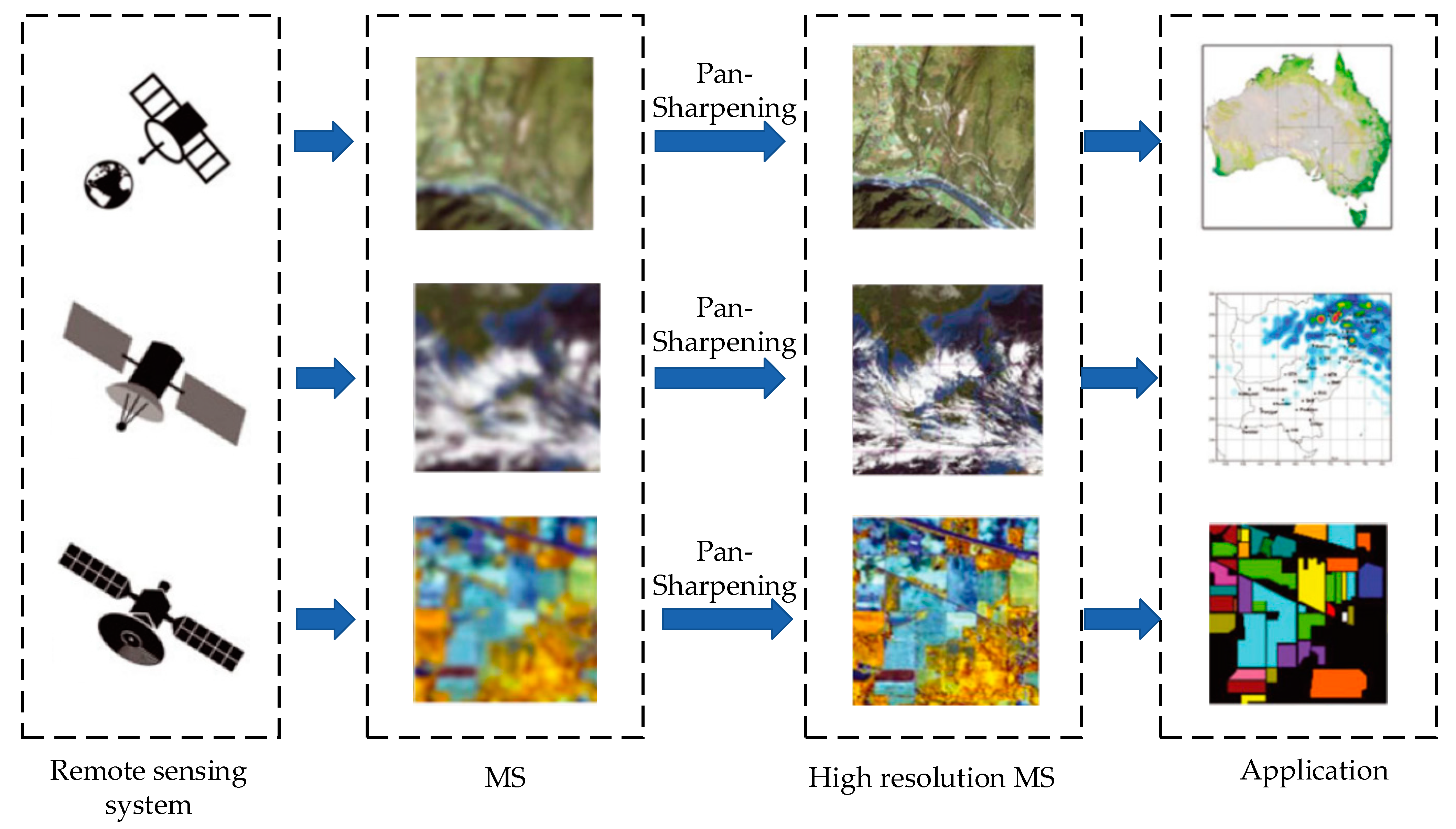
:1. Introduction
- (1)
- An image matting model is introduced in the fusion process, which can effectively maintain the spectral resolution of the MS image.
- (2)
- A NSST is introduced in the multi-resolution analysis process, which has the advantages of multi-scale, multi-direction, and translation invariance. In addition, the NSST can overcome the pseudo-Gibbs effect when reconstructing images and can capture more feature information of the source image.
- (3)
- The low-frequency components are fused according to an ADMM-based β-divergence NMF method. Moreover, the ADMM-based β-divergence NMF method has a faster convergence speed and better solution results.
- (4)
- The traditional local contrast measure method is improved and a WLCM method is proposed in this paper. Initially, the local contrast measure value is calculated using the median of the neighborhood. Then, the mean of the difference between the local pixel values and the middle pixel value is introduced to weight the local contrast measure value. The WLCM method can enhance the faint spatial details and suppress the irrelevant backgrounds, which in turn improves the detection rate of detailed information and ultimately enhances the fusion effect.
2. Materials and Methods
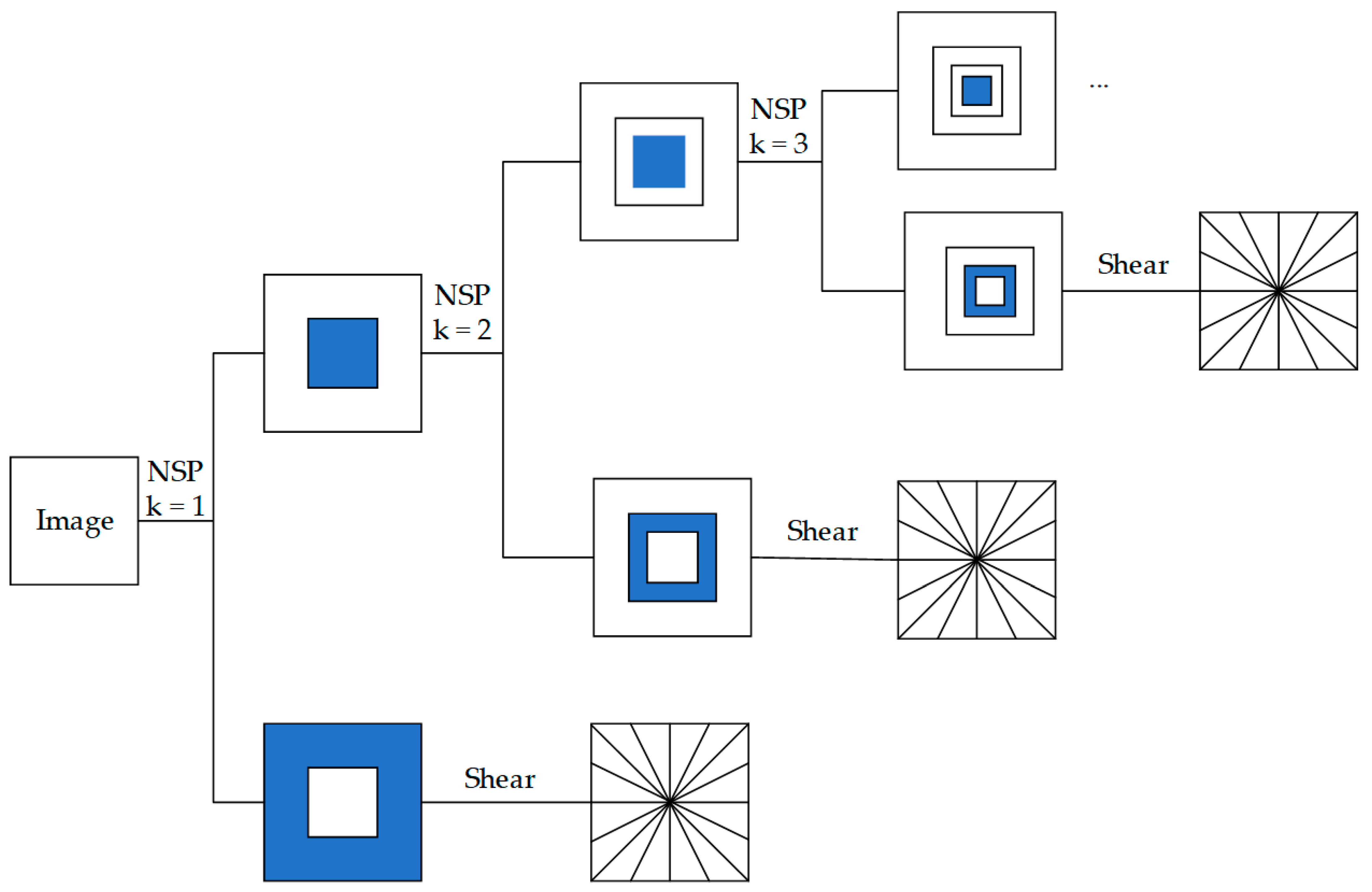
2.1. NSST Decomposition
2.2. Image Matting Model
2.3. β-Divergence Non-Negative Matrix Factorization Based on Alternating Direction Method of Multiplier
| Algorithm 1 The ADMM-based β-divergence NMF | |
| Inputs | E |
| Initialize | |
| Repeat | |
| Until | |
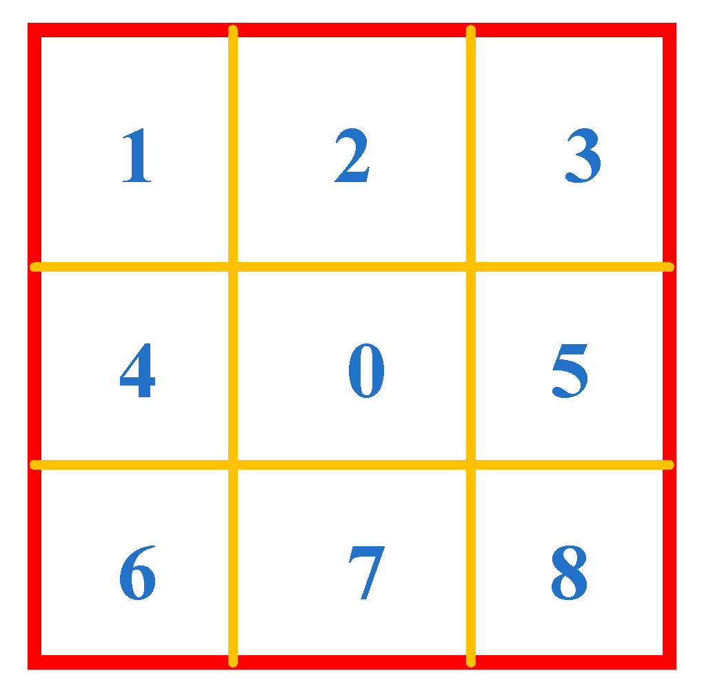
2.4. Weighted Local Contrast Measure
3. The Steps and Principles
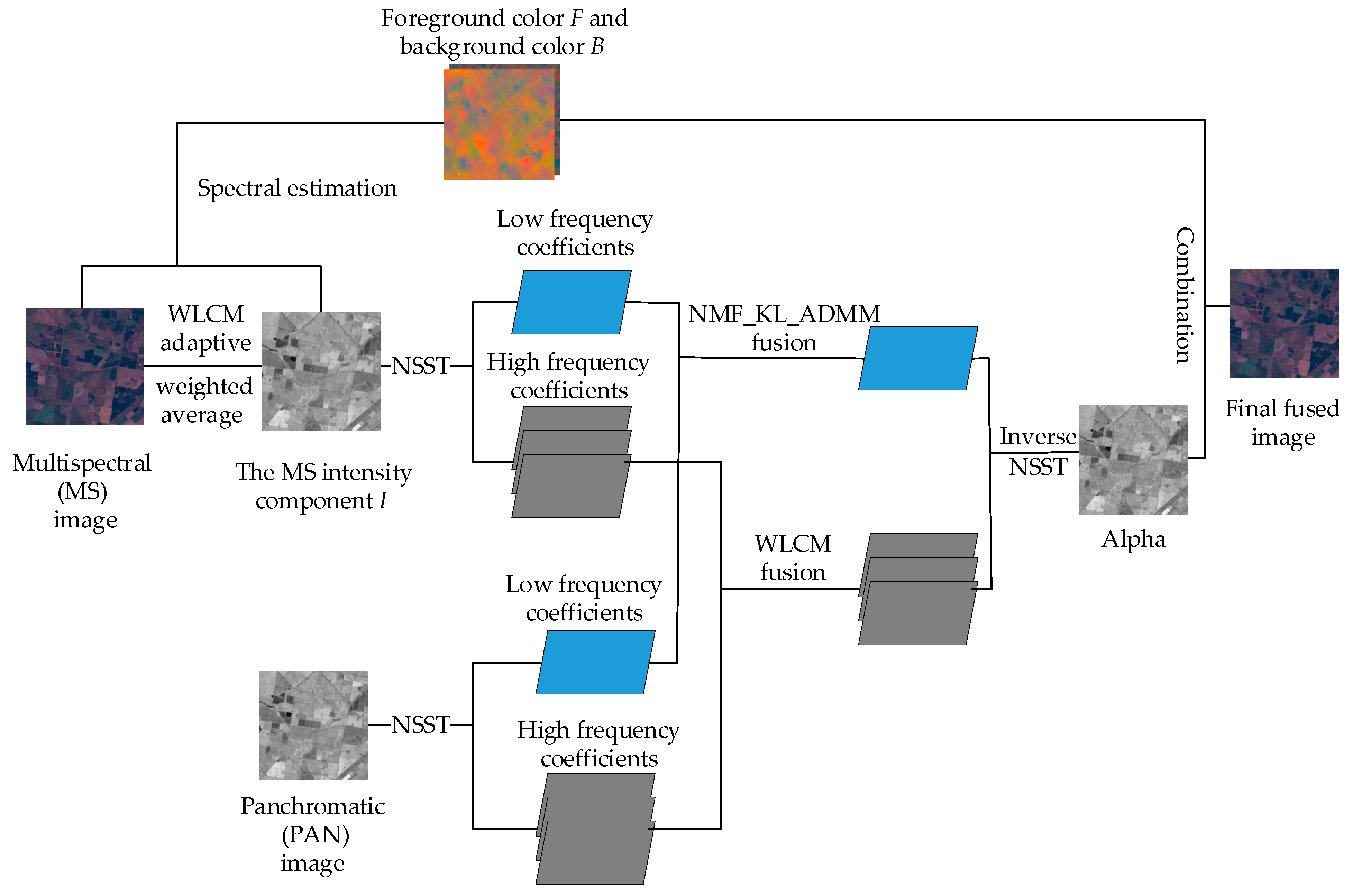
3.1. The Overall Image Fusion Steps
- (1)
- Adaptive Weighted Average Calculates the MS Intensity Component
- (2)
- Spectral Estimation
- (3)
- NSST Decomposition
- (4)
- High-Frequency Components Fusion
- (5)
- Low-Frequency Components Fusion
- (6)
- NSST Inverse Transformation
- (7)
- Image Reconstruction
3.2. High-Frequency Components Fusion Algorithm
3.3. Low-Frequency Component Fusion Algorithm
- (1)
- The low-frequency components LA and LB are sorted into column vectors according to the priority of the rows. Then, the column vectors XA and XB are obtained. If the sizes of LA and LB are both M × N, the sizes of XA and XB are MN × l. The details are as follows:
- (2)
- According to the column vectors XA and XB, the following original matrix X is constructed, and its size is MN × 2.
- (3)
- We set k = 1. NMF is the factorization with error, which means . In order to obtain an approximate factorization and minimize the reconstruction error between X and WH, a cost function must be defined. The cost function can measure the approximation effect of the solution. In the proposed method, we choose Kullback–Leibler (KL) divergence as the cost function. The maximum number of iterations is set to 2000. The initial iteration values W0 and H0 are randomly generated with sizes M × k and k × N, respectively. The details are as follows:
- (4)
- After setting the relevant parameters, the original matrix X is decomposed using an ADMM-based β-divergence NMF method. The detailed iterative process can be found in Section 2.3. When the iteration is finished, the basis matrix W and the weight coefficient matrix H can be obtained. W contains the overall features of the low-frequency components LA and LB, which can be regarded as the approximate reproduction of the original image.
- (5)
- We reset W to a matrix S of M × N. Finally, S is the fusion result of the low-frequency components.
4. Experiments and Discussion
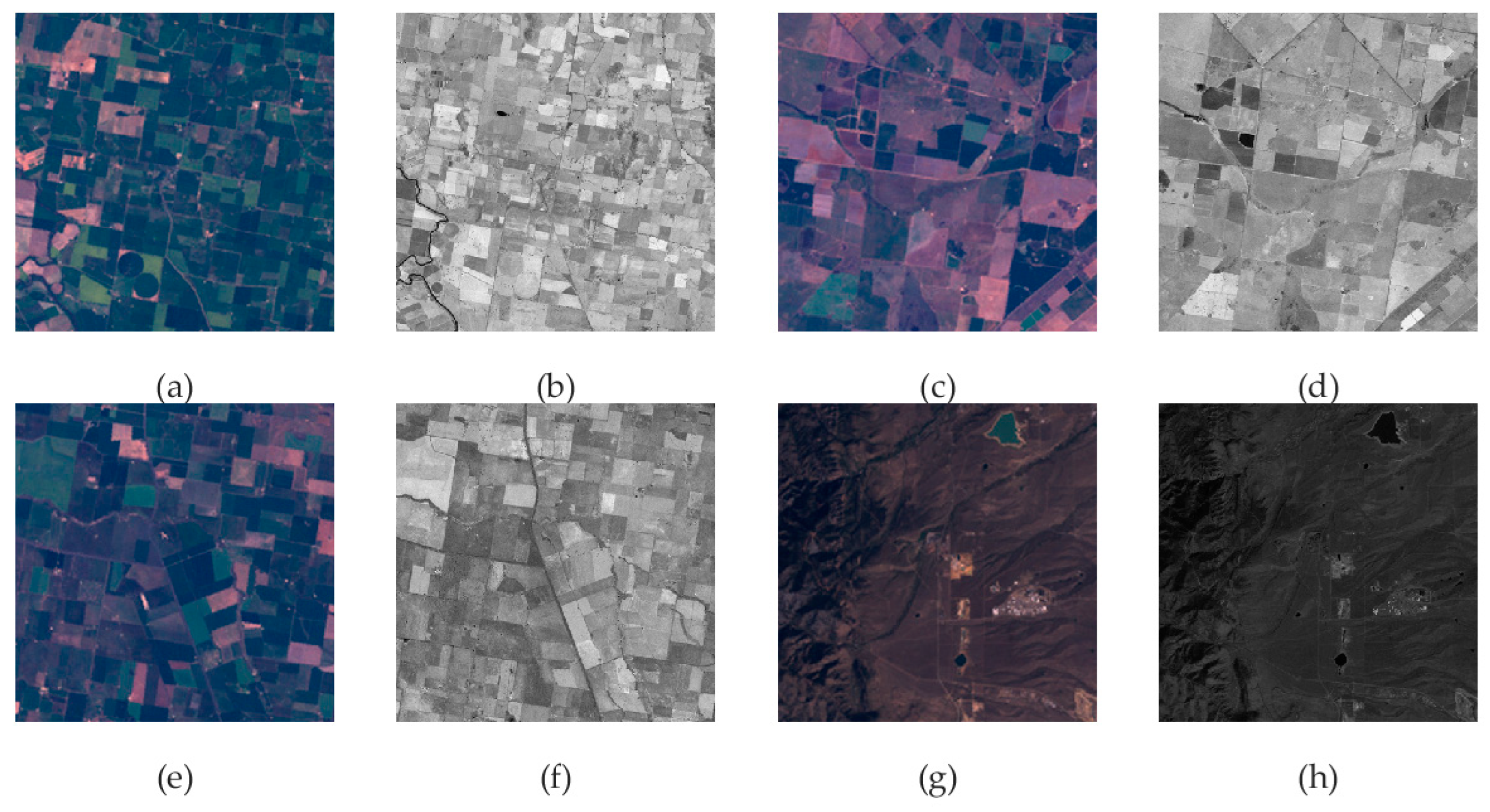
4.1. Experimental Images
4.2. Selected Comparison Method
4.3. Objective Evaluation Indices
- (1)
- The Correlation Coefficient (CC) [21] calculates the correlation between the reference image and a pan-sharpening result. Its ideal value is 1. It is defined as follows:
- (2)
- Erreur Relative Global Adimensionnelle de Synthse (ERGAS) [22] can measure the fusion quality of a pan-sharpening method, which is defined as follows:
- (3)
- Relative Average Spectral Error (RASE) [24] reflects the average performance of a pan-sharpening method on spectral errors. Smaller values of RASE denote less spectral distortion. Its ideal value is 0. It is defined as follows:
- (4)
- (5)
- No Reference Quality Evaluation (QNR) [26] can evaluate the quality of a pan-sharpening image without a reference image, which consists of three parts: a spectral distortion index Dλ, a spatial distortion index Ds, and a global QNR value. The detailed definition is provided in Formula (27). For the global QNR, the higher the value, the better the fusion effect. Its ideal value is 1. Please refer to the literature [26] for more details.
- (6)
- Dλ is a sub-metric of QNR, which can measure the spectral distortion of a pan-sharpening image. The smaller the value, the better the fusion effect. Its ideal value is 0. It is defined as follows:
- (7)
- Ds is a sub-metric of QNR, which can measure the spatial distortion of the fused image. The smaller the value, the better the fusion effect. Its ideal value is 0. It is defined as follows:
4.4. Implementation Details
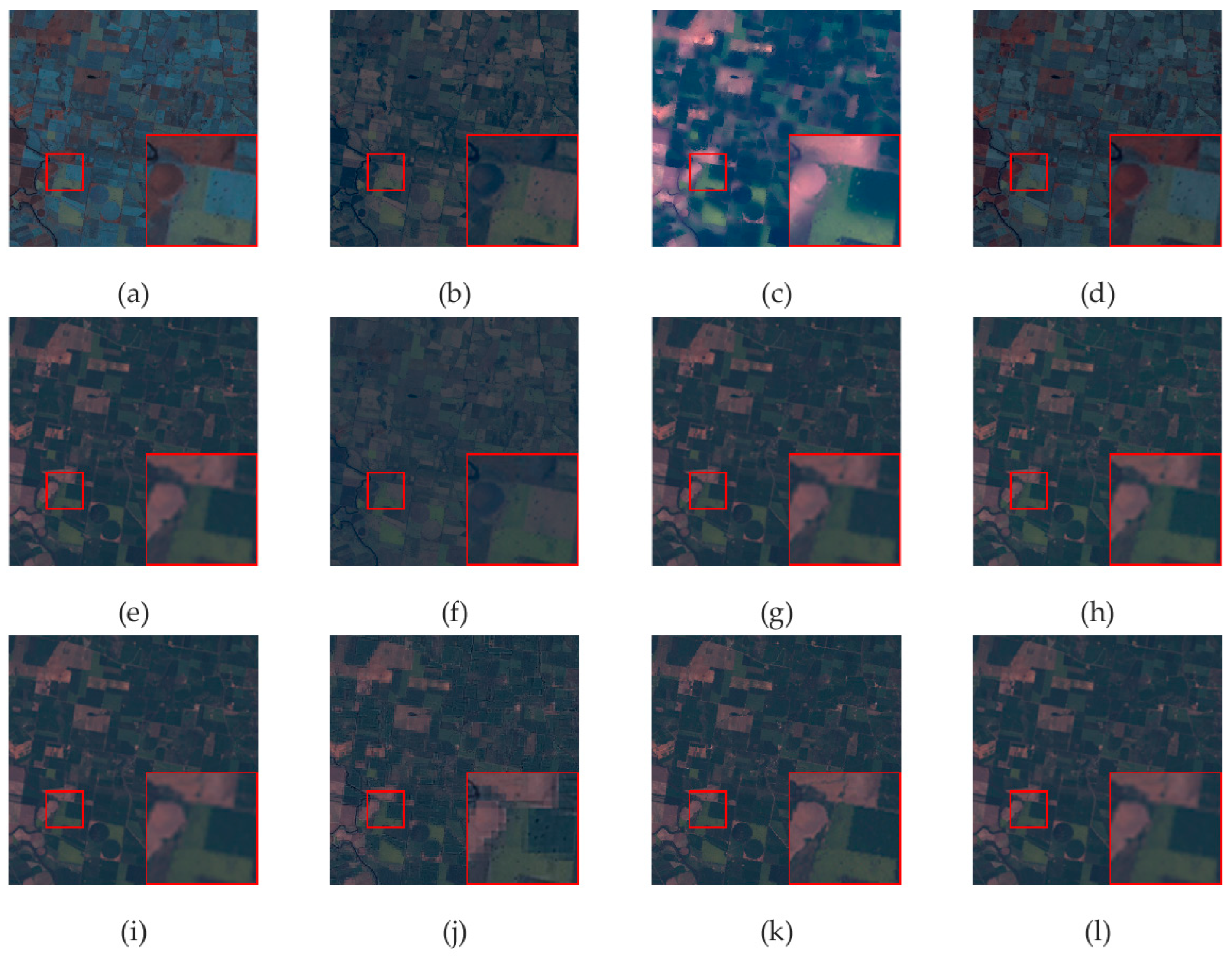
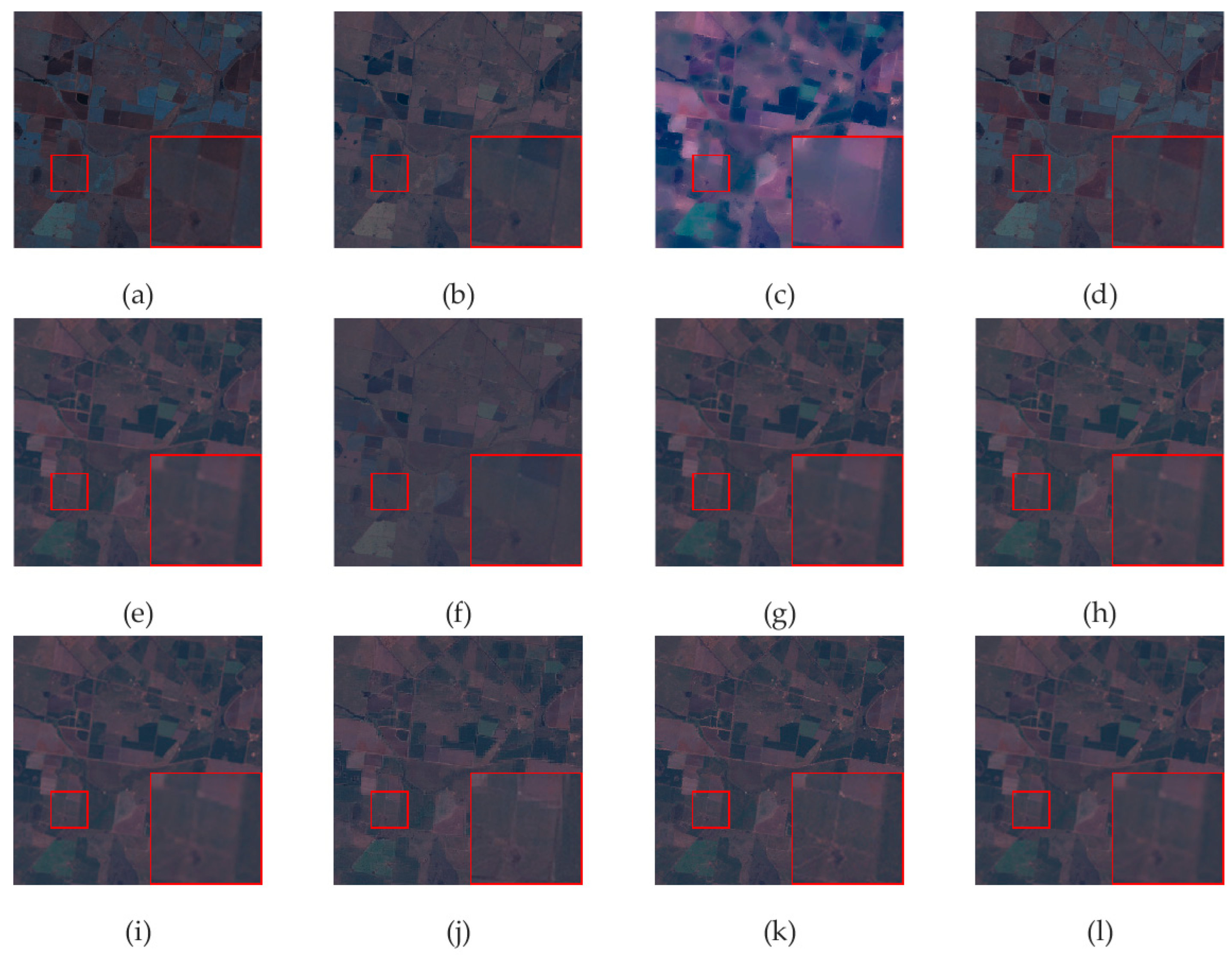
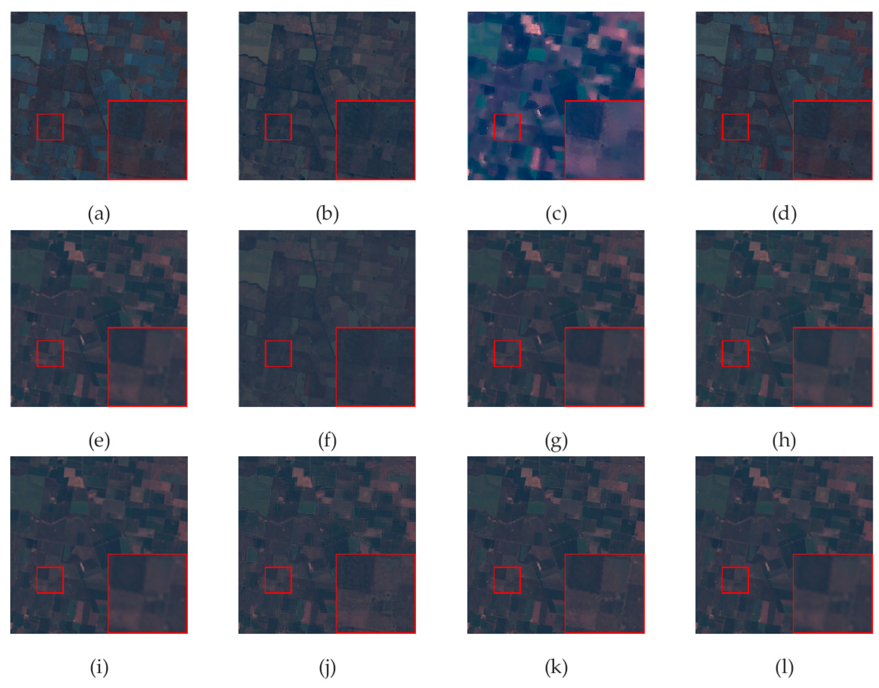
4.5. Experimental Results and Analysis
5. Conclusions
Author Contributions
Funding
Data Availability Statement
Acknowledgments
Conflicts of Interest
References
- Masoudi, R.; Kabiri, P. New intensity-hue-saturation pan-sharpening method based on texture analysis and genetic algorithm-adaption. J. Appl. Remote Sens. 2014, 8, 083640. [Google Scholar] [CrossRef]
- Jelének, J.; Kopačková, V.; Koucká, L.; Mišurec, J. Testing a modified PCA-based sharpening approach for image fusion. Remote Sens. 2016, 8, 794. [Google Scholar] [CrossRef] [Green Version]
- Liu, C.; Qi, X.; Zhang, W.; Huang, X. Research of improved Gram-Schmidt image fusion algorithm based on IHS transform. Eng. Surv. Mapp. 2018, 27, 9–14. [Google Scholar]
- Aiazzi, B.; Baronti, S.; Selva, M. Improving component substitution pansharpening through multivariate regression of MS + Pan data. IEEE Trans. Geosci. Remote Sens. 2007, 45, 3230–3239. [Google Scholar] [CrossRef]
- Vivone, G. Robust band-dependent spatial-detail approaches for panchromatic sharpening. IEEE Trans. Geosci. Remote Sens. 2019, 57, 6421–6433. [Google Scholar] [CrossRef]
- Choi, J.; Yu, K.; Kim, Y. A new adaptive component-substitution based satellite image fusion by using partial replacement. IEEE Trans. Geosci. Remote Sens. 2011, 49, 295–309. [Google Scholar] [CrossRef]
- Cheng, J.; Liu, H.; Liu, T.; Wang, F.; Li, H. Remote sensing image fusion via wavelet transform and sparse representation. ISPRS J. Photogramm. Remote Sens. 2015, 104, 158–173. [Google Scholar] [CrossRef]
- Otazu, X.; Gonzalez-Audicana, M.; Fors, O.; Nunez, J. Introduction of sensor spectral response into image fusion methods. Application to wavelet-based methods. IEEE Trans. Geosci. Remote Sens. 2005, 43, 2376–2385. [Google Scholar] [CrossRef] [Green Version]
- Fu, X.; Lin, Z.; Huang, Y.; Ding, X. A variational pan-sharpening with local gradient constraints. In Proceedings of the IEEE/CVF Conference on Computer Vision and Pattern Recognition, Long Beach, CA, USA, 15–20 June 2019. [Google Scholar]
- Wu, L.; Yin, Y.; Jiang, X.; Cheng, T. Pan-sharpening based on multi-objective decision for multi-band remote sensing images. Pattern Recognit. 2021, 118, 108022. [Google Scholar] [CrossRef]
- Khan, S.S.; Ran, Q.; Khan, M.; Ji, Z. Pan-sharpening framework based on laplacian sharpening with Brovey. In Proceedings of the 2019 IEEE International Conference on Signal, Information and Data Processing (ICSIDP), Chongqing, China, 11–13 December 2019. [Google Scholar]
- Li, Q.; Yang, X.; Wu, W.; Liu, K.; Jeon, G. Pansharpening multispectral remote-sensing images with guided filter for monitoring impact of human behavior on environment. Concurr. Comput. Pract. Exp. 2021, 32, e5074. [Google Scholar] [CrossRef]
- Yin, M.; Liu, W.; Zhao, X.; Yin, Y.; Guo, Y. A novel image fusion algorithm based on nonsubsampled shearlet transform. Optik 2014, 125, 2274–2282. [Google Scholar] [CrossRef]
- Ullah, H.; Ullah, B.; Wu, L.; Abdalla, F.Y.; Ren, G.; Zhao, Y. Multi-modality medical images fusion based on local-features fuzzy sets and novel sum-modified-Laplacian in non-subsampled shearlet transform domain. Biomed. Signal Process. Control 2020, 57, 101724. [Google Scholar] [CrossRef]
- Levin, A.; Lischinski, D.; Weiss, Y. A closed-form solution to natural image matting. IEEE Trans. Pattern Anal. Mach. Intell. 2008, 30, 228–242. [Google Scholar] [CrossRef] [PubMed] [Green Version]
- Sun, D.L.; Fevotte, C. Alternating direction method of multipliers for non-negative matrix factorization with the beta-divergence. In Proceedings of the 2014 IEEE International Conference on Acoustics, Speech and Signal Processing (ICASSP), Florence, Italy, 4–9 May 2014; pp. 6201–6205. [Google Scholar]
- Ghadimi, E.; Teixeira, A.; Shames, I.; Johansson, M. On the optimal step-size selection for the alternating direction method of multipliers. IFAC Proc. 2012, 45, 139–144. [Google Scholar] [CrossRef] [Green Version]
- Chen, C.L.P.; Li, H.; Wei, Y.; Xia, T.; Tang, Y.Y. A local contrast method for small infrared target detection. IEEE Trans. Geosci. Remote Sens. 2013, 52, 574–581. [Google Scholar] [CrossRef]
- Jin, X.; Jiang, Q.; Yao, S.; Zhou, D.; Nie, R.; Lee, S.-J.; He, K. Infrared and visual image fusion method based on discrete cosine transform and local spatial frequency in discrete stationary wavelet transform domain. Infrared Phys. Technol. 2018, 88, 1–12. [Google Scholar] [CrossRef]
- US Gov. Available online: https://earthexplorer.usgs.gov/ (accessed on 24 October 2019).
- Alparone, L.; Wald, L.; Chanussot, J.; Thomas, C.; Gamba, P.; Bruce, L. Comparison of pansharpening algorithms: Outcome of the 2006 GRS-S data-fusion contest. IEEE Trans. Geosci. Remote Sens. 2007, 45, 3012–3021. [Google Scholar] [CrossRef] [Green Version]
- Zhang, L.; Zhang, L.; Tao, D.; Huang, X. On combining multiple features for hyperspectral remote sensing image classification. IEEE Trans. Geosci. Remote Sens. 2012, 50, 879–893. [Google Scholar] [CrossRef]
- Yang, Y.; Tong, S.; Huang, S.; Lin, P. Multifocus image fusion based on NSCT and focused area detection. IEEE Sens. J. 2015, 15, 2824–2838. [Google Scholar]
- Ranchin, T.; Wald, L. Fusion of high spatial and spectral resolution images: The ARSIS concept and its implementation. Photogramm. Eng. Remote Sens. 2000, 66, 49–61. [Google Scholar]
- Chang, C.-I. Spectral information divergence for hyperspectral image analysis. In Proceedings of the IEEE 1999 International Geoscience and Remote Sensing Symposium. IGARSS’99 (Cat. No.99CH36293), Hamburg, Germany, 28 June–2 July 1999; Volume 1, pp. 509–511. [Google Scholar]
- Alparone, L.; Aiazzi, B.; Baronti, S.; Garzelli, A.; Nencini, F.; Selva, M. Multispectral and panchromatic data fusion assessment without reference. Photogramm. Eng. Remote Sens. 2008, 74, 193–200. [Google Scholar] [CrossRef] [Green Version]
- Wang, Z.; Bovik, A.C. A universal image quality index. IEEE Signal Process. Lett. 2002, 9, 81–84. [Google Scholar] [CrossRef]


| Projects | Implementation Details |
|---|---|
| The number of band-pass directional sub-bands in each layer of NSST | 32, 32, 16, 16 |
| The level of NSST directional decomposition | 4 |
| Experimental environment | Windows 10 System PC Intel (R) Core (TM) i7-8700 CPU 3.20 GHz 16 GB Memory |
| Development platform | MATLAB R2018a |
| CC (1) | ERGAS (0) | SID (0) | RASE (0) | QNR (1) | |
|---|---|---|---|---|---|
| BT | 0.320 | 6.684 | 0.060 | 28.735 | 0.384 |
| GSA | 0.113 | 7.504 | 0.065 | 26.255 | 0.151 |
| GF | 0.857 | 7.612 | 0.011 | 20.597 | 0.868 |
| IHS | 0.364 | 6.130 | 0.029 | 26.130 | 0.397 |
| MOD | 0.944 | 1.605 | 0.007 | 5.148 | 0.904 |
| PCA | 0.173 | 6.241 | 0.049 | 26.641 | 0.258 |
| PRACS | 0.944 | 1.607 | 0.008 | 5.175 | 0.916 |
| VLGC | 0.945 | 1.602 | 0.009 | 5.156 | 0.902 |
| BDSD-PC | 0.942 | 1.613 | 0.007 | 5.160 | 0.884 |
| WT | 0.734 | 3.054 | 0.021 | 11.238 | 0.573 |
| Proposed | 0.948 | 1.486 | 0.005 | 4.923 | 0.925 |
| CC (1) | ERGAS (0) | SID (0) | RASE (0) | QNR (1) | |
|---|---|---|---|---|---|
| BT | 0.317 | 5.800 | 0.018 | 22.405 | 0.347 |
| GSA | 0.052 | 5.377 | 0.036 | 20.560 | 0.110 |
| GF | 0.876 | 4.145 | 0.009 | 24.917 | 0.802 |
| IHS | 0.325 | 5.717 | 0.011 | 18.624 | 0.386 |
| MOD | 0.944 | 1.618 | 0.006 | 5.320 | 0.904 |
| PCA | 0.128 | 6.241 | 0.031 | 18.624 | 0.199 |
| PRACS | 0.945 | 1.607 | 0.006 | 5.515 | 0.909 |
| VLGC | 0.942 | 1.875 | 0.008 | 5.314 | 0.832 |
| BDSD-PC | 0.946 | 1.613 | 0.007 | 5.460 | 0.918 |
| WT | 0.820 | 1.900 | 0.007 | 7.376 | 0.565 |
| Proposed | 0.949 | 1.324 | 0.004 | 3.817 | 0.930 |
| CC (1) | ERGAS (0) | SID (0) | RASE (0) | QNR (1) | |
|---|---|---|---|---|---|
| BT | 0.386 | 4.090 | 0.019 | 14.609 | 0.397 |
| GSA | 0.109 | 4.945 | 0.034 | 17.795 | 0.133 |
| GF | 0.862 | 7.612 | 0.014 | 20.597 | 0.832 |
| IHS | 0.336 | 4.146 | 0.017 | 14.140 | 0.369 |
| MOD | 0.943 | 1.604 | 0.011 | 5.148 | 0.874 |
| PCA | 0.135 | 4.246 | 0.026 | 15.258 | 0.223 |
| PRACS | 0.941 | 1.607 | 0.011 | 3.875 | 0.849 |
| VLGC | 0.934 | 1.613 | 0.008 | 5.156 | 0.870 |
| BDSD-PC | 0.942 | 1.602 | 0.011 | 5.160 | 0.869 |
| WT | 0.794 | 1.986 | 0.009 | 7.369 | 0.572 |
| Proposed | 0.946 | 1.218 | 0.006 | 2.952 | 0.882 |
| CC (1) | ERGAS (0) | SID (0) | RASE (0) | QNR (1) | |
|---|---|---|---|---|---|
| BT | 0.810 | 8.302 | 0.010 | 21.254 | 0.617 |
| GSA | 0.818 | 3.260 | 0.005 | 12.917 | 0.610 |
| GF | 0.890 | 8.412 | 0.006 | 20.597 | 0.804 |
| IHS | 0.814 | 3.464 | 0.009 | 12.584 | 0.606 |
| MOD | 0.943 | 1.612 | 0.003 | 5.153 | 0.839 |
| PCA | 0.827 | 3.537 | 0.005 | 14.013 | 0.621 |
| PRACS | 0.929 | 2.056 | 0.003 | 8.143 | 0.743 |
| VLGC | 0.945 | 1.602 | 0.004 | 5.156 | 0.839 |
| BDSD-PC | 0.950 | 1.593 | 0.003 | 5.140 | 0.845 |
| WT | 0.905 | 2.286 | 0.005 | 9.098 | 0.824 |
| Proposed | 0.953 | 1.370 | 0.002 | 2.103 | 0.982 |
Publisher’s Note: MDPI stays neutral with regard to jurisdictional claims in published maps and institutional affiliations. |
© 2022 by the authors. Licensee MDPI, Basel, Switzerland. This article is an open access article distributed under the terms and conditions of the Creative Commons Attribution (CC BY) license (https://creativecommons.org/licenses/by/4.0/).
Share and Cite
Pan, Y.; Liu, D.; Wang, L.; Benediktsson, J.A.; Xing, S. A Pan-Sharpening Method with Beta-Divergence Non-Negative Matrix Factorization in Non-Subsampled Shear Transform Domain. Remote Sens. 2022, 14, 2921. https://doi.org/10.3390/rs14122921
Pan Y, Liu D, Wang L, Benediktsson JA, Xing S. A Pan-Sharpening Method with Beta-Divergence Non-Negative Matrix Factorization in Non-Subsampled Shear Transform Domain. Remote Sensing. 2022; 14(12):2921. https://doi.org/10.3390/rs14122921
Chicago/Turabian StylePan, Yuetao, Danfeng Liu, Liguo Wang, Jón Atli Benediktsson, and Shishuai Xing. 2022. "A Pan-Sharpening Method with Beta-Divergence Non-Negative Matrix Factorization in Non-Subsampled Shear Transform Domain" Remote Sensing 14, no. 12: 2921. https://doi.org/10.3390/rs14122921