Estimation of Regional Ground-Level PM_2.5 Concentrations Directly from Satellite Top-of-Atmosphere Reflectance Using A Hybrid Learning Model

Abstract

The accurate prediction of PM_2.5 concentrations is important for environmental protection. The accuracy of the commonly used prediction methods is not high; so, this paper proposes a PM_2.5 concentration prediction method based on a hybrid learning model. The Top-of-Atmosphere Reflectance (TOAR), PM_2.5 data decomposed by wavelets, and meteorological data were used as input features to build an integrated prediction model using random forest and LightGBM, which was applied to PM_2.5 concentration prediction in the Beijing–Tianjin–Hebei region. The practical application showed that the proposed method using TOAR, incorporating wavelet decomposition with meteorological element data, had an improvement of 0.06 in the R² of the model accuracy and a reduction of 2.93 and 1.14 in the root mean square error (RMSE) and mean absolute error (MAE), respectively, over the model using Aerosol Optical Depth (AOD). Our model had a prediction accuracy of R² of 0.91, which was better than the other models. We used this model to estimate and analyze the variation in PM_2.5 concentrations in the Beijing–Tianjin–Hebei region, and the results were the same as the actual PM_2.5 concentration distribution trend. Obviously, the proposed model has a high prediction accuracy and can avoid the errors caused by the limitations of the AOD inversion method.

1. Introduction

PM_2.5 has a large impact on atmospheric environmental quality and can cause health problems [1,2,3]. Compared with PM10, PM_2.5 has a small particle size, large area, and strong activity; it can remain in the atmosphere for a long time and be transmitted over long distances [4]. 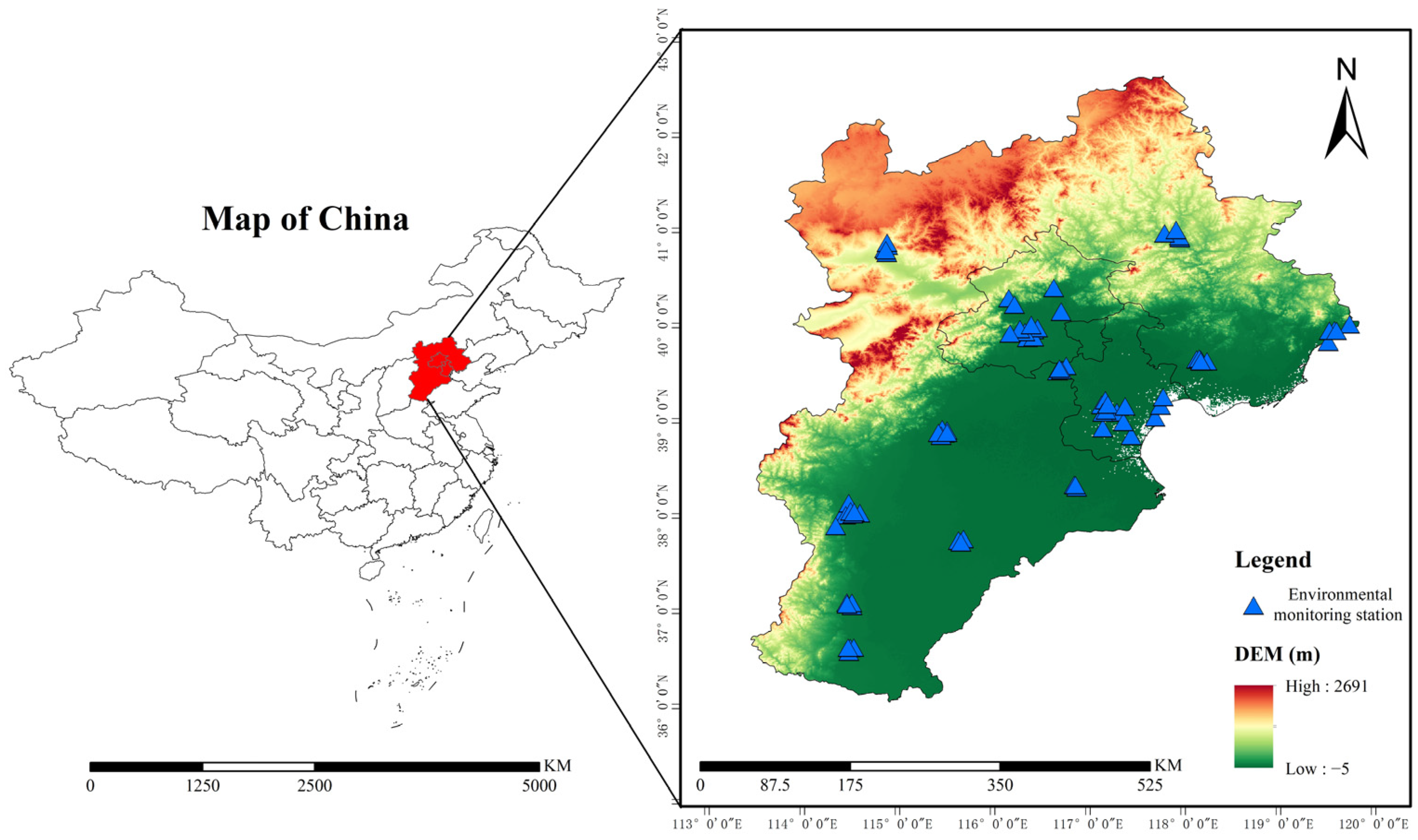Particles with a diameter of 10 microns usually deposit in the upper respiratory tract, while those below 2 microns can enter the human alveoli, directly affecting the ventilation function of the lungs, causing the body to be in a state of oxygen deprivation [5]. With the rapid development of the economy, industrial production and human-caused emissions have increased dramatically, resulting in a serious deterioration in air quality in east-central China, with the Beijing–Tianjin–Hebei region being the most significantly affected area [6,7].

The conventional monitoring method is to establish ground monitoring stations [8], and by January 2015, more than 1500 PM_2.5 concentration (unit: µg/m³) observation stations had been built nationwide to obtain ground-level high-precision PM_2.5 concentrations. However, the ground monitoring stations are restricted by human and material resource conditions, resulting in the uneven distribution of monitoring points, lack of regional representativeness, and lack of continuity of data [9,10]. In recent years, many studies have shown that, compared with traditional air pollution monitoring technology, remote sensing [11] has the advantages of a wide monitoring range, fast and easy to achieve continuous monitoring, and unique ways to acquire environmental information [12].

Aerosol optical depth (AOD) has been widely and successfully used for PM_2.5 concentration estimation due to its different spatial resolution and its close correlation with particle concentrations [13,14,15]. Many researchers have developed different models establishing a link between satellite AOD and ground PM_2.5 concentrations, including physical models [16], statistical models, and machine learning models. The physical models, based on the physical relationship between AOD and PM_2.5, use higher quality AOD to assess PM_2.5 concentrations. Tang et al. [17] used Landsat8 OLI images to develop a physical model of the relationship between AOD and PM_2.5. However, the aerosol patterns need to be determined with long-term ground-based monitoring data, which has an impact on PM_2.5 estimates. Statistical models used to describe the linear relationship between AOD and PM_2.5 have evolved from a single linear model to a linear mixed-effects model [18] and a geographically and temporally weighted regression (GTWR) model [19]. He et al. [20] developed an improved geographically and temporally weighted regression (iGTWR) model that considered the seasonal characteristics of the data to obtain the AOD–PM_2.5 relationship to predict PM_2.5 concentrations in the Beijing–Tianjin–Hebei region, with an R² of 0.82 after cross-validation. Chu et al. [21] proposed to combine geographically and temporally weighted regression (GTWR) and random sample consistency (RANSAC), which resulted in a good fit between AOD and PM_2.5. However, the statistical model could not accurately respond to the complex nonlinear relationship between the variables and PM_2.5, which limited the accuracy of the inversion of PM_2.5.

Compared with statistical models, machine learning models, including random forest, gradient boosting, and deep learning [22], can better handle nonlinear problems, which can provide a more accurate estimation of PM_2.5 concentrations. Li et al. [23] combined random forest with AOD to monitor PM_2.5 concentrations in the Beijing–Tianjin–Hebei region, which was advantageous in dealing with the complex nonlinear relationships between a large number of meteorological elements and atmospheric pollutants. Wei et al. [24] proposed a tree-based spatial–temporal lightweight gradient boosting model with the inclusion of parameters such as meteorological elements, population density, land utilization, and ground elevation for national hourly PM_2.5 concentration prediction. The prediction results achieved an R² of 0.85 and an RMSE and MAE of 13.62 and 8.49, respectively, and the proposed method outperformed most traditional statistical regression models and tree-based machine learning models.

However, the above studies were all based on satellite AOD data, which are limited in spatial and temporal coverage due to the low revisit rate of satellites and limitations in the application of the AOD inversion methods [25,26], thus affecting the prediction accuracy of PM_2.5. To solve the above problems, Shen et al. [27] used a deep belief network (DBN) to construct a model in which the top-of-atmosphere reflectance (TOAR) from the MODIS sensor inversion AOD band was used instead of AOD for PM_2.5 prediction. The cross-validation yielded an R² of 0.87, which avoided the error in the AOD inversion process and had higher prediction accuracy and spatial coverage. Bai et al. [28] used four different machine learning algorithms (random forest, extreme gradient boosting, gradient augmented regression, and support vector regression) to construct PM_2.5 prediction models based on TOAR and AOD, respectively, and cross-validation yielded the best performance of the TOAR-based random forest model with an R² of 0.75. Yang et al. [29] integrated variables, such as satellite TOAR, meteorological elements, and land utilization, and used a random forest model to estimate PM_2.5 concentrations in the Yangtze River Delta region with a cross-validated R² of 0.92. Yin et al. [30] used the LightGBM algorithm to predict PM_2.5 concentrations nationwide using TOAR and AOD from Himawari-8, and the LightGBM model had an R² of 0.83 in regions where AOD was not available.

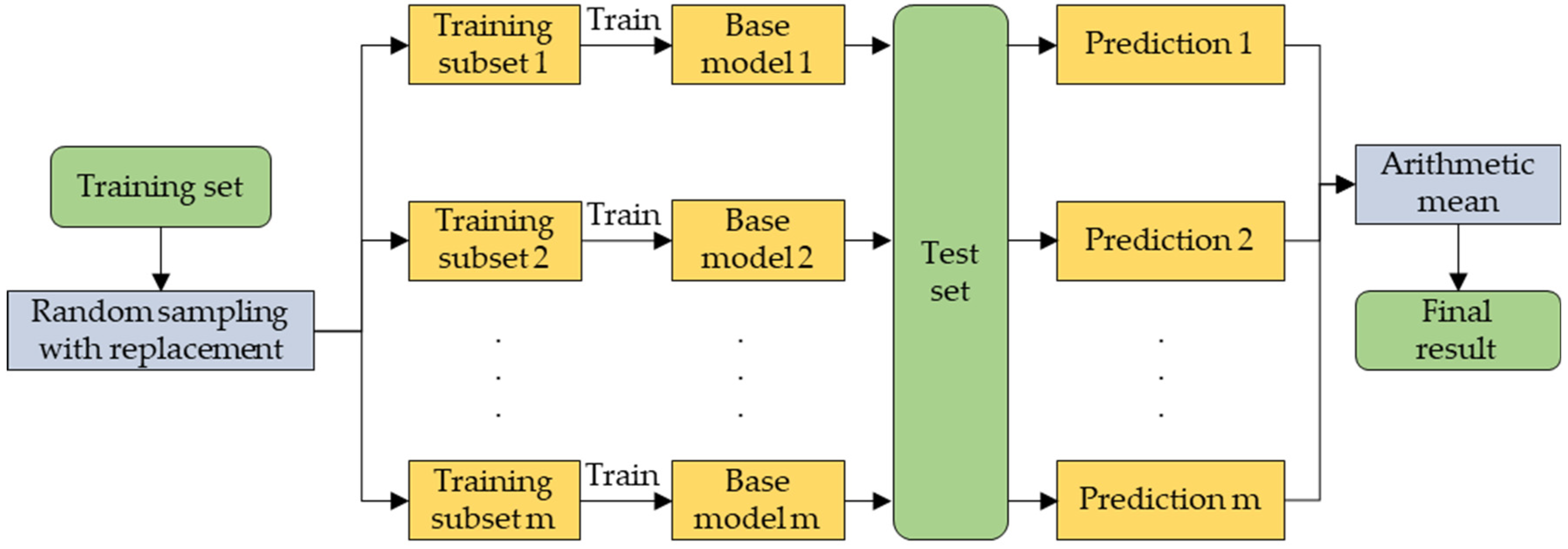
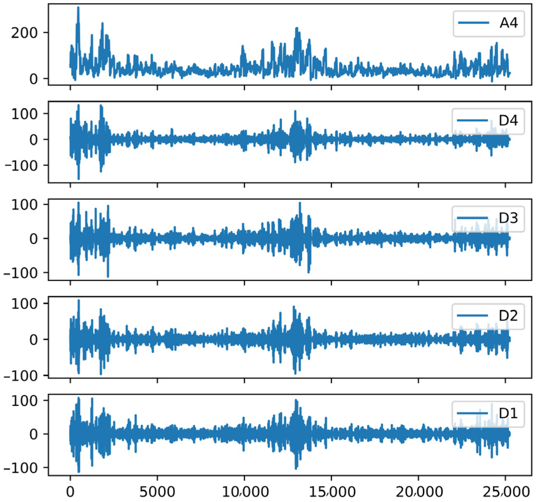
All the above models were single-model predictions, which can lead to poor single-model performance due to various factors such as feature space, model size, and hyperparameter selection, etc. To make up for this deficiency, hybrid models have been created. Hybrid models [31] refer to models generated by combining signal decomposition techniques with other prediction models. The hybrid model is a further decomposition of the nonlinear original time series into more stable and regular subseries, and the final prediction results are obtained by aggregating the predicted values of all subseries. Ding et al. [32] performed wavelet decomposition of meteorological variables and PM_2.5 and used the CatBoost algorithm to build a prediction model for PM_2.5, obtaining an R² of 0.88. Wang et al. 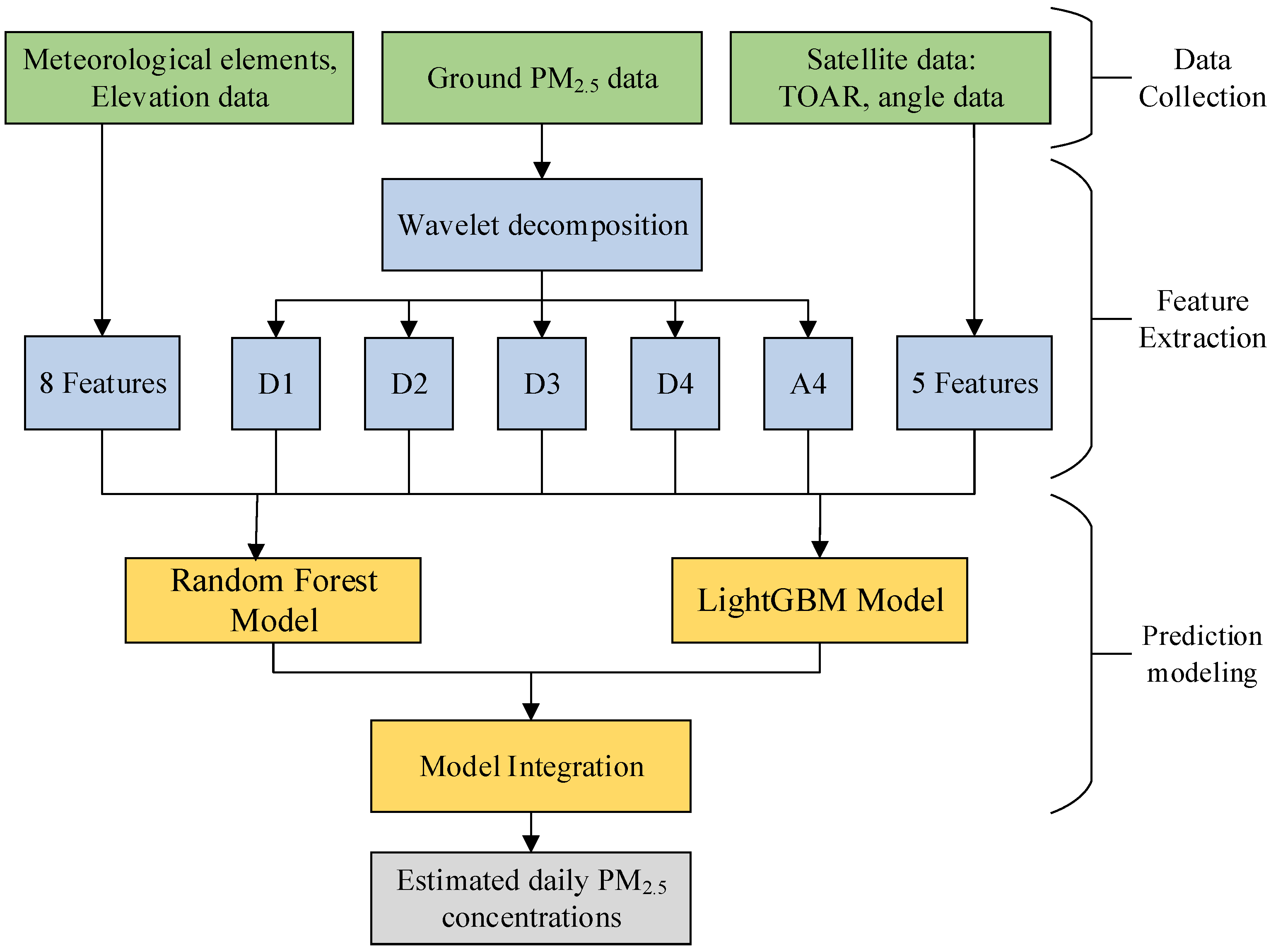[33] performed a four-layer wavelet decomposition of the original PM_2.5 and used the XGBoost algorithm to model each layer of PM_2.5 after wavelet decomposition with an R² of 0.87. Therefore, this study aims to develop a hybrid learning model that uses MODIS 1B satellite TOAR as the main prediction parameter and adds auxiliary parameters such as meteorological elements and elevation data to estimate daily PM_2.5 concentrations in the Beijing–Tianjin–Hebei region.

2. Materials and Methods

2.1. Research Area

The Beijing–Tianjin–Hebei region is located in northern China, with a geographical range between 113.3–119.5 E and 36–42.4 N, including Beijing and Tianjin, two municipalities directly under the central government, as well as 11 prefecture-level cities in Hebei Province and two cities directly under provincial control. The region is the core of the country’s northern economy and the political and cultural center of the country. Figure 1 shows the elevation map of the Beijing–Tianjin–Hebei region, which is rapidly industrializing and urbanizing, with increasing pollutant emissions and serious air pollution problems. Since the region connects to the Yanshan Mountains to the north and the Taihang Mountains to the west, these will have a blocking and weakening effect on the wind, resulting in pollutants not being easily dispersed, which will seriously affect the public health and economic development of the region.

2.2. Data Collection

This study used PM_2.5 concentration data, satellite remote sensing data, meteorological elements, and ground elevation data as variables for model fitting and validation.

(1)

Near-ground PM_2.5 monitoring data

The near-ground PM_2.5 data included data from 80 state-controlled monitoring stations in the Beijing–Tianjin–Hebei region for the two years 2019 and 2020, which are available on the website of the Shanghai Environmental Monitoring Center (https://data.epmap.org/product, accessed on 1 September 2021). The invalid data (PM_2.5 concentrations ≤ 0 μg/m³) and missing data (None) were removed before data integration.

(2)

Satellite Data

The satellite data used Terra MODIS 1B calibration radiometric data (MOD021KM); MODIS (Moderate Resolution Imaging Spectoradiometer) is currently carried on Terra and Aqua satellites with a spatial resolution of 1KM and is available for free download at URL https://ladsweb.modaps.eosdis.nasa.gov/, accessed on 2 September 2021. PM_2.5 prediction models were constructed using observation angles (solar zenith angle, solar azimuth angle, satellite zenith angle, and satellite azimuth angle) and the TOAR in band 1 (0.62–0.67 μm), band 3 (0.459–0.479 μm), and band 7 (2.105–2.155 μm). At the same time, MODIS AOD data with a resolution of 1 KM over two years were downloaded as model inputs for comparison.

(3)

Meteorological and elevation data

The meteorological data were obtained from the ERA-Interim reanalysis in the ECMWF (European Center of Middle-range Weather Forecast). The meteorological data included seven meteorological variables: Boundary Layer Height (BLH; unit: m), atmospheric Surface Pressure (SP; unit: hPa), Total Column of Water (TCW), Total Column Ozone (TCO), 2 m air temperature (unit: K), U/V wind speed at 10 m (U10M, V10M; unit: ms⁻¹), where “U10M” and “V10M” were vector synthesized. Using the daily average meteorological quantities at zero point in the Beijing–Tianjin–Hebei region, consistent with PM_2.5 concentrations and satellite data, the selection of meteorological elements was based on previous studies [34,35], which revealed factors that have a significant impact on PM_2.5 concentrations. The elevation data of the Beijing–Tianjin–Hebei region were obtained from the Geographic State Monitoring Cloud Platform (http://www.dsac.cn/, accessed on 6 October 2021). All meteorological data were resampled to the same spatial resolution (1KM) as the satellite data, and the processed dataset was used for model development.

(4)

Descriptive Statistics

The dataset mainly included PM_2.5 concentrations data, satellite data, and auxiliary data, as shown in

Table 1. Descriptive statistics of the dataset.

Category	Variable	Spatial Resolution	Temporal Resolution
PM2.5	daily-mean PM2.5	—	day
Remote sensing data	TOAR, AOD, solar zenith, solar azimuth, sensor zenith, sensor azimuth	1 km	day
		1 km	day
		1 km	day
Meteorological element data	Boundary Layer Height, Total Column of Water, Total Column Ozone, Surface Pressure, 2 m temperature, 10 m u-component of wind, 10 m v-component of wind	0.25	day
Auxiliary data	Elevation data	1 km	year

.

The daily maximum PM_2.5 concentrations in the Beijing–Tianjin–Hebei region were 424 μg/m³, and the average daily average PM_2.5 concentrations at each site were higher than 75 μg/m³ for 53 days per year. According to Chinese standards, air quality with PM_2.5 concentrations below 35 μg/m³ is excellent, below 75 μg/m³ is good, and above 75 μg/m³ will be harmful to the human body and reach the level of pollution. The seasonal averages of PM_2.5 concentrations in the Beijing–Tianjin–Hebei region throughout the study period were: winter (69.70 μg/m³) > spring (40.31 μg/m³) > autumn (37.83 μg/m³) > summer (31.26 μg/m³). Among them, the annual average PM_2.5 concentrations in Beijing were lower (39 μg/m³), and the annual average PM_2.5 concentrations in Tianjin (50 μg/m³) were higher than that in Beijing. The annual average TOAR of B1, B3, and B7 measured by MOD021KM products were 0.18, 0.22, and 0.11, respectively.

2.3. Methods

In the PM_2.5 concentration prediction study, the main processes were data collection, feature extraction, and prediction modeling, and Figure 2 shows the technology roadmap.

(1)

Data collection: This included temporal and spatial matching of ground station PM_2.5 data, satellite data, and meteorological element data;

(2)

Feature extraction: Four layers of wavelet decomposition were used to obtain four high-frequency detail components (D1, D2, D3, and D4) and one low-frequency approximate component A4 for PM_2.5 data, and the features were mainly composed of D1-D4, A4, meteorological elements, elevation data, TOAR, and angle data with a total of 18 features;

(3)

Prediction modeling: The predictions of the PM_2.5 subseries data after wavelet decomposition were summed using Random Forest (RF) and LightGBM models to construct an integrated learning model to obtain the final prediction results of the PM_2.5 concentrations.

2.3.1. Feature Extraction

The model input features included near-ground PM_2.5 data, satellite data, meteorological elements, and elevation data, where wavelet decomposition was used to decompose the PM_2.5 data to obtain high frequency and low frequency components.

Wavelet decomposition [36] can separate high-frequency signals from trending low frequency signals to obtain more data features. The decomposition process is as follows:

$$\{\begin{array}{l}{A}_{j+1}=H\left(A_j\right)\hfill \\ D_{j+1}=G\left(D_j\right)\hfill \end{array}$$

(1)

where $A_j$ and $D_j$ refer to the low frequency approximation component and high frequency detail component, respectively, $j$ is the number of layers of wavelet decomposition, $H$ is the low-pass filter, and $G$ is the high-pass filter.

When performing the wavelet transform, each layer of the decomposed signal is half of the predecomposed signal data; so, two interpolation reconstructions are required to recover the signal length, and the reconstruction equation is as follows:

$$\{\begin{array}{l}{A}_J={\left(H^{\ast }\right)}^j{A}_j\hfill \\ D_J={\left(H^{\ast }\right)}^{j-1}{G}^{\ast }{D}_j\hfill \end{array}$$

(2)

where $H^{\ast }$ and $G^{\ast }$ are the double operators of $H$, $G$ and $J$ is the number of layers of the low-frequency sequence and the high-frequency sequence that recovers the signal length after reconstruction.

Figure 3 is a schematic diagram of the results after the wavelet decomposition of the partial PM_2.5 data, with the number of samples on the horizontal axis and the PM_2.5 concentration values on the vertical axis. It can be seen that the A4 low-frequency series had a clear trend as well as a certain periodicity, while D1–4 reflected the random fluctuation changes in the trend of the original series.

2.3.2. Precision Modeling

Integrated learning improves generalization and robustness through the combination of multiple base learners, including “Bagging” and “Boosting”. In this study, the random forest model in “Bagging” and the LightGBM model in “Boosting” were selected as the base learners to build the hybrid learning model.

(1) Random forest model: random forest [37] builds bagging integration based on decision trees as the base learner and introduces random feature selection in the training process of decision trees. The bagging algorithm randomly samples the samples with replacement, constructs mutually independent sample datasets with equal sample sizes, and trains different models in the same algorithm. For regression problems, it calculates the arithmetic average of the prediction results of all models to obtain the final result. The flowchart of the bagging algorithm is shown in Figure 4.

(2) LightGBM model: both the LightGBM model [38,39] and XGBoost model [40] are gradient boosting frameworks based on decision trees, and the objective function of the XGBoost is Equation (3):

$$O{b}^{\left(t\right)}=\sum _{j=1}^T[G_j{w}_j+\frac{1}{2}\left(H_j+\lambda \right)w_j^2]+\gamma T$$

(3)

where $T$ is the total number of leaf nodes in the t tree, $G_j$ and $H_j$ are the cumulative sum of the first-order and second-order partial derivatives of the samples contained in leaf node j, respectively. $\lambda$ and $\gamma$ are constants; $w_j$ is the score value of the j leaf node.

It is worth noting that LightGBM has the same gain $G_j{w}_j+\frac{1}{2}\left(H_j+\lambda \right)w_j^2$ as XGBoost, but LightGBM uses a histogram-based algorithm to speed up the training process, as well as strategies such as leaf-wise growth with depth restrictions and Gradient-based One-Side Sampling (GOSS), which allows LightGBM to have a higher prediction accuracy and less running memory.

In Random Forest and LightGBM, different combinations of hyperparameters lead to models with large gaps in prediction performance, and since both models have more hyperparameters, it is necessary to automatically search for the combination of hyperparameters with the best performance. In this study, the Bayesian optimization method [41] was selected to optimize the main hyperparameters of the random forest and LightGBM models. The flowchart of the Bayesian optimization algorithm is shown in Figure 5.

(3) Model integration: in model training, the results obtained from the random forest model predictions are denoted as $X=\{X_1,X_2,X_3,\dots ,X_n\}$, and n is the sequence length; the predicted result of the LightGBM model is denoted as $Y=\{Y_1,Y_2,Y_3,\dots ,Y_n\}$, and the actual PM_2.5 concentrations data are denoted as $Z=\{Z_1,Z_2,Z_3,\dots ,Z_n\}$. The linear regression model $Z=aX+bY+c$ of $Z$ and $X$, $Y$ was constructed, where a, b, and c are the regression model coefficients.

(4) Evaluation Indicators

The mean absolute error (MAE), root mean square error (RMSE), and goodness of fit (R²) were used to evaluate the model performance, and the MAE, RMSE, and R² expressions are shown in Equations (4)–(6).

$$\mathrm{MAE}=\frac{1}{n}\sum _{i=1}^n\mid y_{true}-y_{predict}\mid$$

(4)

$$\mathrm{RMSE}=\sqrt{\frac{1}{n}\sum _{i=1}^n{\left(y_{true}-y_{predict}\right)}^2}$$

(5)

$${\mathrm{R}}^2=1-\frac{{\displaystyle \sum _{i=1}^n}{\left(y_{true}-y_{predict}\right)}^2}{{\displaystyle \sum _{i=1}^n}{\left(y_{true}-y_{average}\right)}^2}$$

(6)

where $y_{true}$, $y_{predict}$, and $y_{average}$ are the true, predicted, and average values of PM_2.5, respectively, and n is the overall length of the data.

In summary, the hybrid learning model proposed in this paper mainly includes the following four steps.

Step 1. We performed wavelet decomposition on the PM_2.5 sample data from ground stations and matched the decomposed high-frequency and low-frequency subseries of each layer with TOAR, meteorological elements, and elevation data in space and time.

Step 2. The random forest and LightGBM models were used for training, and the optimal hyperparameter combinations of the random forest and LightGBM models were selected by the Bayesian optimization algorithm to obtain the final random forest and LightGBM models.

Step 3. We integrated the above two models to obtain the hybrid learning model and evaluated the model performance using MAE, RMSE, and R² as the evaluation metrics of the model.

Step 4. The PM_2.5 concentrations in the Beijing–Tianjin–Hebei region were predicted using the hybrid learning model, and the spatial and temporal distributions of PM_2.5 concentrations in the Beijing–Tianjin–Hebei region were plotted.

3. Results

3.1. PM_2.5 Concentrations Prediction and Comparative Analysis

3.1.1. Application Environment and Parameter Setting

The experimental environment was a PC with the following configuration: Windows 10 64 bit, Intel Core i7–7500 U CPU@2.70 GHz,4 GRAM, simulation using Anaconda Navigator3 (Jupyter notebook), and python 3.7 for the experimental platform.

The random forest model and LightGBM model selected in this study both contain more parameters; so, the Bayesian optimization method was selected to find the best of the main hyperparameters in the random forest and LightGBM models, where the best hyperparameter combinations of the optimized random forest model are shown in

Table 2. Optimal hyperparameters of the random forest model.

Name	Meaning	Value
n_estimators	Tree number	949
max_depth	Maximum depth of tree	24
max_features	Number of tree features	0.5
min_samples_split	Conditions limiting the continuation of subtree division	4
min_samples_leaf	Minimum number of samples of leaf nodes	4

, and the best hyperparameter combinations of the LightGBM model are shown in

Table 3. Optimal hyperparameters of the LightGBM model.

Name	Meaning	Value
num_boost_round	Iteration number	1350
max_depth	Maximum depth of tree	16
feature_fraction	Select the set scale feature to build tree	0.84
bagging_fraction	Proportion of data used in each iteration	0.73
min_child_weight	Sum of the minimum leaf node weights	16
reg_alpha	L1 Regularization	0.27
reg_lambda	L2 Regularization	0.33
learning_rate	Learning Rate	0.01

.

The hybrid learning model was obtained by model integration with the expression:

$${\mathrm{PM}}_{2.5HybridModel}=0.4659{\mathrm{PM}}_{2.5RF}+0.6231{\mathrm{PM}}_{2.5LightGBM}-4.1297$$

(7)

3.1.2. Analysis and Comparison of Models with Different Variables Entered

In order to verify the validity of the proposed model, different variables were entered, as shown below, for comparative analysis.

Figure 6 shows the model performance estimates based on TOAR and AOD, with and without the inclusion of wavelet decomposition and meteorological element data.

Table 4. Model design and performance.

	Feature	Wavelet Decomposition	Meteorological Elements	R2	RMSE	MAE
(a)	TOAR	yes	yes	0.9138	11.6008	7.3444
(b)	AOD	yes	yes	0.8507	14.5302	8.4794
(c)	TOAR	no	yes	0.9061	12.1086	7.8400
(d)	AOD	no	yes	0.8430	14.8983	8.9637
(e)	TOAR	yes	no	0.8205	15.9296	9.6845
(f)	AOD	yes	no	0.8149	17.0038	10.4776
(g)	TOAR	no	no	0.8030	16.6905	10.3785
(h)	AOD	no	no	0.8095	17.2508	10.8727

shows the design and performance of the model. Figure 6a,b show the models with both meteorological elements and wavelet decomposition; the R², RMSE, and MAE of Figure 6b were 0.85, 14.53, and 8.48, respectively. Compared with Figure 6b, the R², RMSE, and MAE of Figure 6a were 0.91, 11.60, and 7.34, respectively, indicating that the TOAR-based model can effectively improve the PM_2.5 prediction accuracy, which is due to the use of TOAR data, avoiding the uncertainty in the AOD inversion process.

In the absence of meteorological elements, the prediction performance of each model decreased, but the prediction accuracy of PM_2.5 using wavelet decomposition was higher than that of the model without wavelet decomposition, for example, in Figure 6e,g, because wavelet decomposition can separate high-frequency signals with high-frequency detail features from trending low-frequency signals, thus obtaining more data features and decomposing PM_2.5 data into more stable and regular subseries.

3.1.3. Analysis and Comparison of Different Models

To further demonstrate the reliability of the model proposed in this study, we compared the cross-validation results of the proposed model with the more popular regression models currently available, including multiple linear regression (MLR), geographically and temporally weighted regression, random forest, LightGBM, XGBoost, CatBoost, and DBN. The above model was used to construct PM_2.5 concentration prediction models based on TOAR, while adding wavelet decomposition and meteorological elements to estimate PM_2.5 concentrations in the Beijing–Tianjin–Hebei region in 2020. As shown in

Table 5. Comparing the performance of different models for PM_2.5 concentration estimation in the Beijing–Tianjin–Hebei region in 2020.

Model	R2	RMSE	MAE
MLR	0.2440	34.4142	23.3809
GTWR	0.3193	32.6560	21.7422
RF 1	0.8892	13.1518	8.0969
LightGBM	0.8943	12.8470	8.5899
WD 2 + XGBoost	0.8897	13.1197	8.4524
WD + CatBoost	0.8801	13.6810	8.5159
DBN	0.8596	14.7267	9.7049
This study	0.9090	12.3642	7.3717

¹ RF: Random Forest. ² WD: Wavelet Decomposition.

, the PM_2.5 prediction accuracy of the machine learning models was higher than that of the multiple linear regression and geographically and temporally weighted regression models, and the advantage of the random forest over other tree-based models was that the number of trees in the forest was minimal, and LightGBM required less memory and less time than the other models. Therefore, in this study, Random Forest and LightGBM were selected to build a hybrid model, which obtained a higher prediction accuracy than other machine learning models, with the highest R² and the lowest RMES and MAE.

At the same time, we selected studies that also used MODIS sensors for PM_2.5 daily concentration estimation for comparative analysis (

Table 6. Comparison of the performance of different models for PM_2.5 daily concentration estimation based on MODIS sensor.

Model	Primary Predictor	Spatial Resolution	Scale	Performance			Reference
				R2	RMSE	MAE
Two-stage	AOD	10 KM	YRD 1	0.78	19.18	—	Hua et al. (2019) [42]
RF	AOD	10 KM	BTH 2	0.84	25.32	—	Li et al. (2019) [23]
GTWR	AOD	3 KM	China	0.80	18.00	12.03	He et al. (2018) [43]
IGTWR	AOD	3 KM	BTH	0.84	27.84	—	He et al. (2018) [20]
WT + XGBoost	AOD	3 KM	YRD	0.87	12.83	8.97	Wang et al. (2022) [33]
LME	AOD	1 KM	BTH	0.85	21.49	15.26	Xue et al. (2021) [44]
STRF	AOD	1 KM	China	0.85	15.57	9.77	Wei et al. (2019) [45]
WT + CatBoost	AOD	1 KM	BTH	0.88	17.79	—	Ding et al. (2021) [32]
SIDLM	TOAR	3 KM	China	0.70	15.30	—	Yan et al. (2021) [22]
DBN	TOAR	1 KM	Wuhan	0.87	9.89	—	Shen et al. (2018) [27]
This study	TOAR	1 KM	BTH	0.91	12.36	7.37	—

¹ YRD: Yangtze River Delta region. ² BTH: Beijing–Tianjin–Hebei region.

). It can be seen from Table 6 that (a) our study was higher than other studies ([20,22,23,33,42,43]) in spatial resolution (1 KM); (b) at present, most studies were based on AOD for PM_2.5 concentrations estimation, and we used TOAR as the main parameter for PM_2.5 concentration estimation. In terms of other studies with the same 1 KM resolution, the prediction accuracy of this study was higher than that of most existing studies ([27,32,44,45]). The results show that the satellite TOAR-based hybrid learning model proposed in this study outperformed most models in the estimation and prediction of PM_2.5 concentrations.

3.2. Spatial and Temporal Distribution of PM_2.5 Concentrations

3.2.1. Seasonal Distribution

In order to better observe the evolution of PM_2.5 concentrations, the four-season distribution of PM_2.5 concentrations in the Beijing–Tianjin–Hebei region in 2020 was studied. Figure 7 shows the seasonal distribution of PM_2.5 concentrations observed at 80 ground-based monitoring stations in the Beijing–Tianjin–Hebei region throughout the study period, with March–May in spring, June–August in summer, September–November in autumn, and December–February in winter. The PM_2.5 concentrations at most monitoring points south of Yanshan Mountain and Taihang Mountain were higher than those in the northern part of the mountains, firstly, because of the blocking effect of the mountains, resulting in a lower diffusion of pollutants and, secondly, because of the higher altitude and fewer human activities, thus leading to a reduction in pollutant emissions.

From Figure 7, it can be seen that the PM_2.5 concentrations in the Beijing–Tianjin–Hebei region had obvious seasonal differences, with the highest concentration in winter, which was significantly higher than the other three seasons, with the lowest concentration in summer. The reasons for this include the rapid growth in pollutants in winter due to the use of heating, which leads to the burning of coal. Meanwhile, the model had comparable effects using TOAR and AOD in spring, summer, and autumn, but the prediction model using AOD had larger errors in winter, which is due to the seasonal limitation of the inversion method of AOD, especially in winter. As can be seen from Figure 8, the R², RMSE, and MAE using TOAR were better than the model using AOD under the same conditions. This is due to two main problems with MODIS-based AOD products at present: first, as a sensor on a polar-orbiting satellite, AOD monitoring information can only be obtained twice a day; second, because the inversion of AOD is affected by seasons and regions. Statistics show that the annual average coverage of AOD in the Yangtze River Delta region of China was only 40% in 2013–2014 and only 25% in summer, due to the influence of cloud cover and snow accumulation [46]. In contrast, TOAR from satellites was used in this study for PM_2.5 concentration estimation directly, which effectively avoided the intermediate process of AOD inversion, and the temporal resolution of TOAR is hourly. Therefore, TOAR has a wider spatial coverage compared with AOD, and in the areas where AOD is missing, TOAR can be used to better predict PM_2.5 concentrations and provide more reliable prediction results.

3.2.2. PM_2.5 Concentrations in Selected Key Regions

Three pollution hotspots in the Beijing–Tianjin–Hebei region, namely Beijing, Tianjin, and Shijiazhuang, were selected to further analyze the regional spatio–temporal estimation capability of the proposed hybrid learning model. Among the three regions, the annual average PM_2.5 concentrations were highest in Shijiazhuang (52.98 μg/m³), followed by Tianjin with annual average PM_2.5 concentrations of 49.93 μg/m³ and the lowest annual average concentration in Beijing (39.07 μg/m³); Figure 9 shows the daily observed PM_2.5 time series and the predicted PM_2.5 concentrations values obtained for the three polluted regions in 2020, and the results show that the proposed hybrid model accurately estimated PM_2.5 concentrations in all monitoring stations, even when there was severe pollution.

Daily PM_2.5 concentrations can reveal more details of changes than annual average PM_2.5 concentrations and seasonal average PM_2.5 concentrations. We chose the day with the highest PM_2.5 concentrations in the three regions in 2020 and analyzed it together with meteorological elements. The meteorological elements included boundary layer height, surface pressure, and temperature, which are highly correlated with PM_2.5 concentrations. Figure 10 shows the PM_2.5 concentrations and the corresponding meteorological conditions in Beijing (12 February 2020), Tianjin (27 January 2020), and Shijiazhuang (15 January 2020), respectively. The highest annual PM_2.5 concentrations in all three regions were in winter, which coincides with the seasonal characteristics analyzed in Figure 7. As shown in Figure 10, the model-estimated PM_2.5 concentrations were highly correlated with the meteorological conditions, and the trend of PM_2.5 concentrations increased with the increase in surface pressure, temperature, and boundary layer height.

4. Discussion

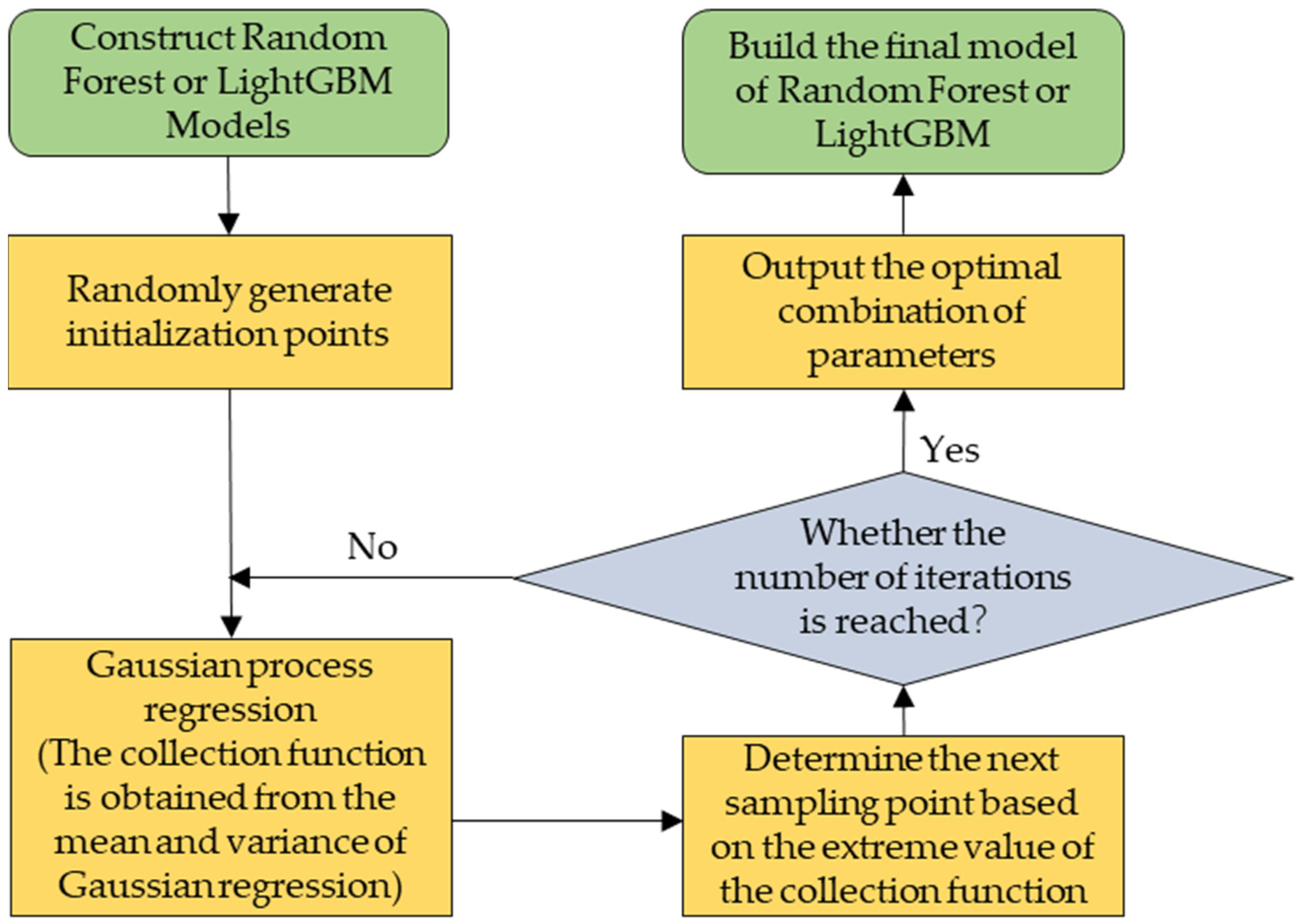
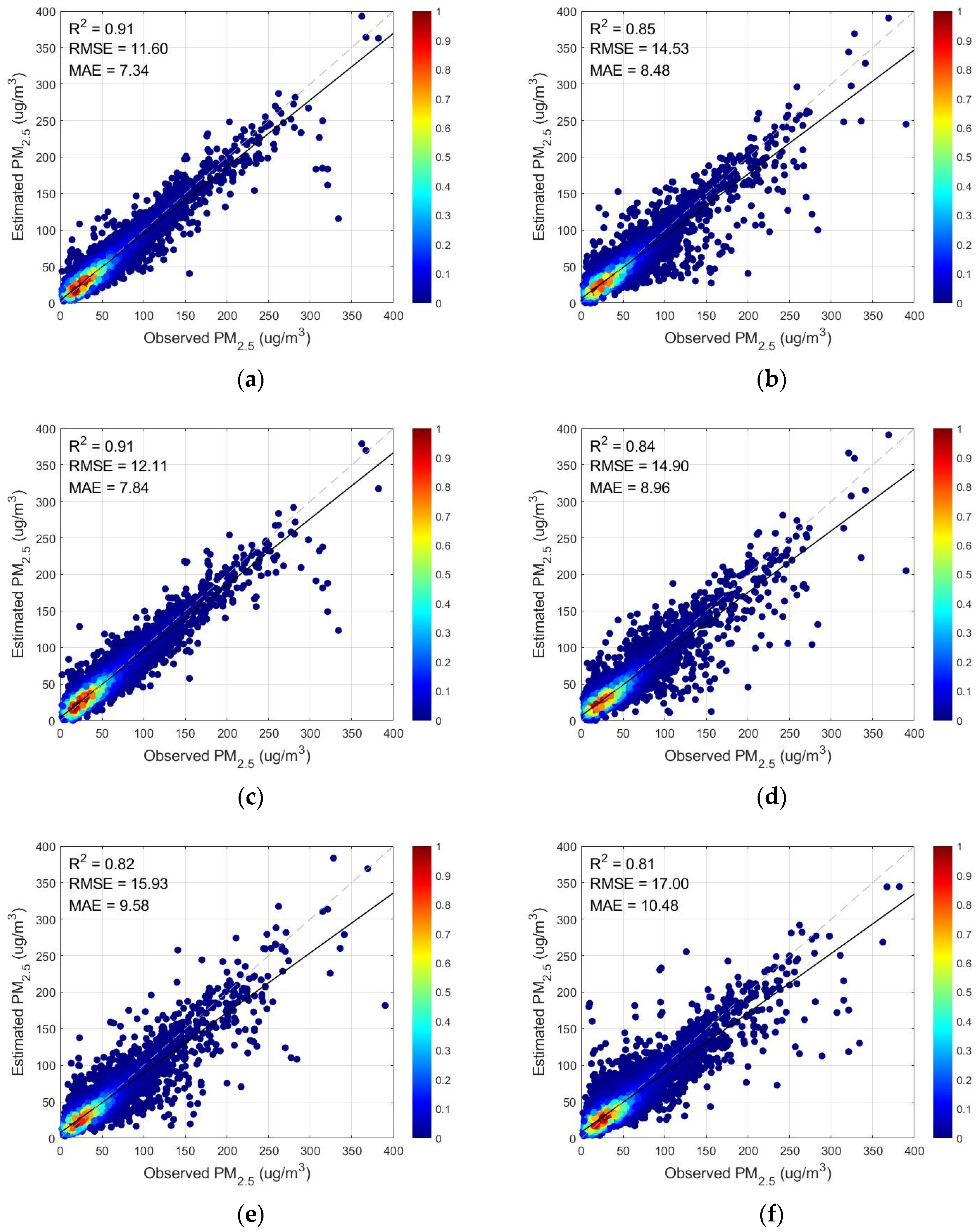
In this study, we proposed a hybrid learning model, which first performed wavelet decomposition of PM_2.5 observations and then constructed an integrated model using Random Forest and LightGBM. The model inputs combined satellite TOAR, meteorological elements, and elevation data and were examined in time and space on daily and seasonal scales for PM_2.5 concentration estimation in the Beijing–Tianjin–Hebei region. 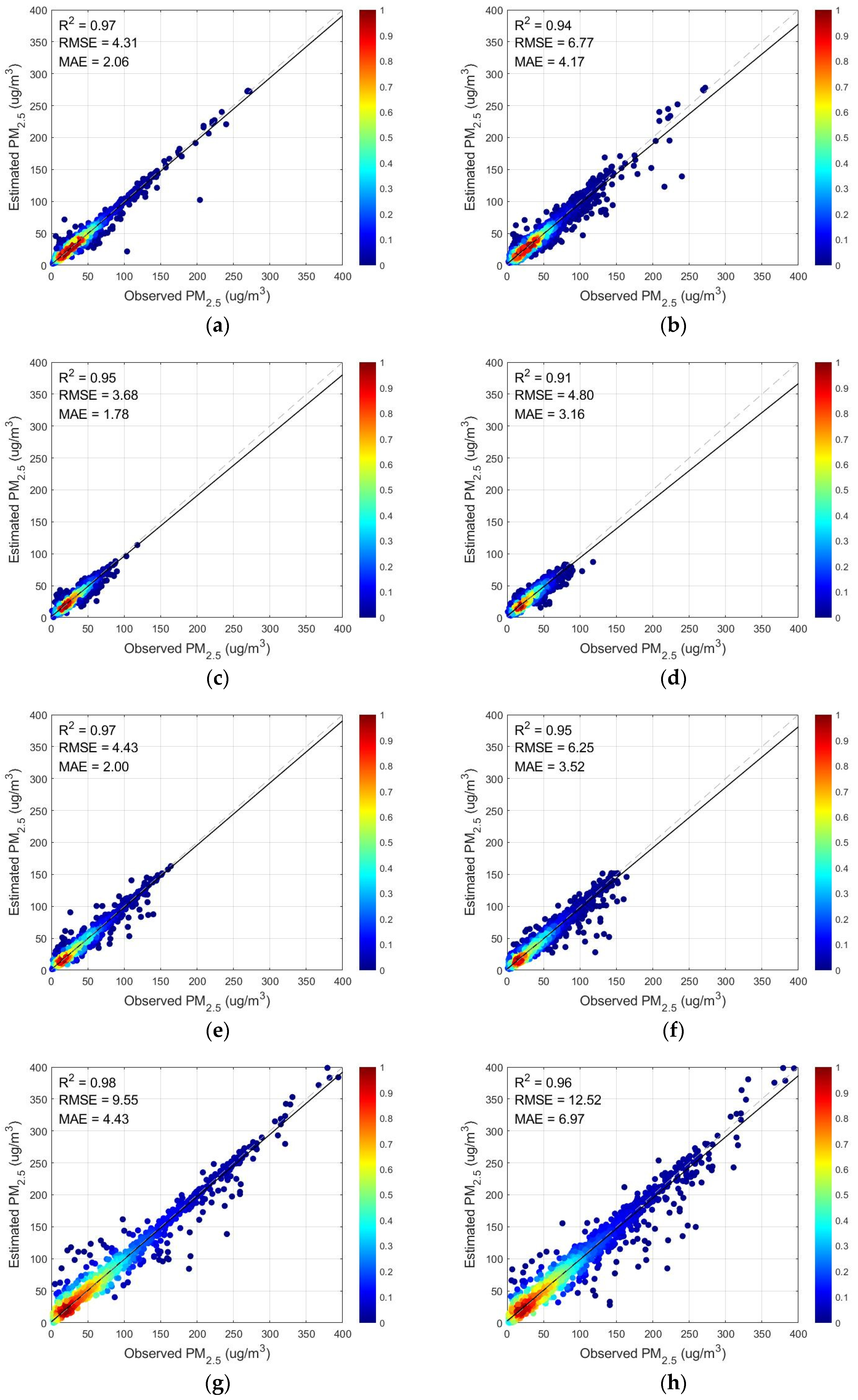The results showed that the estimated and true values were highly consistent, and the time-based cross-validation R², RMSE, and MAE were 0.91, 11.60, and 7.34, respectively. 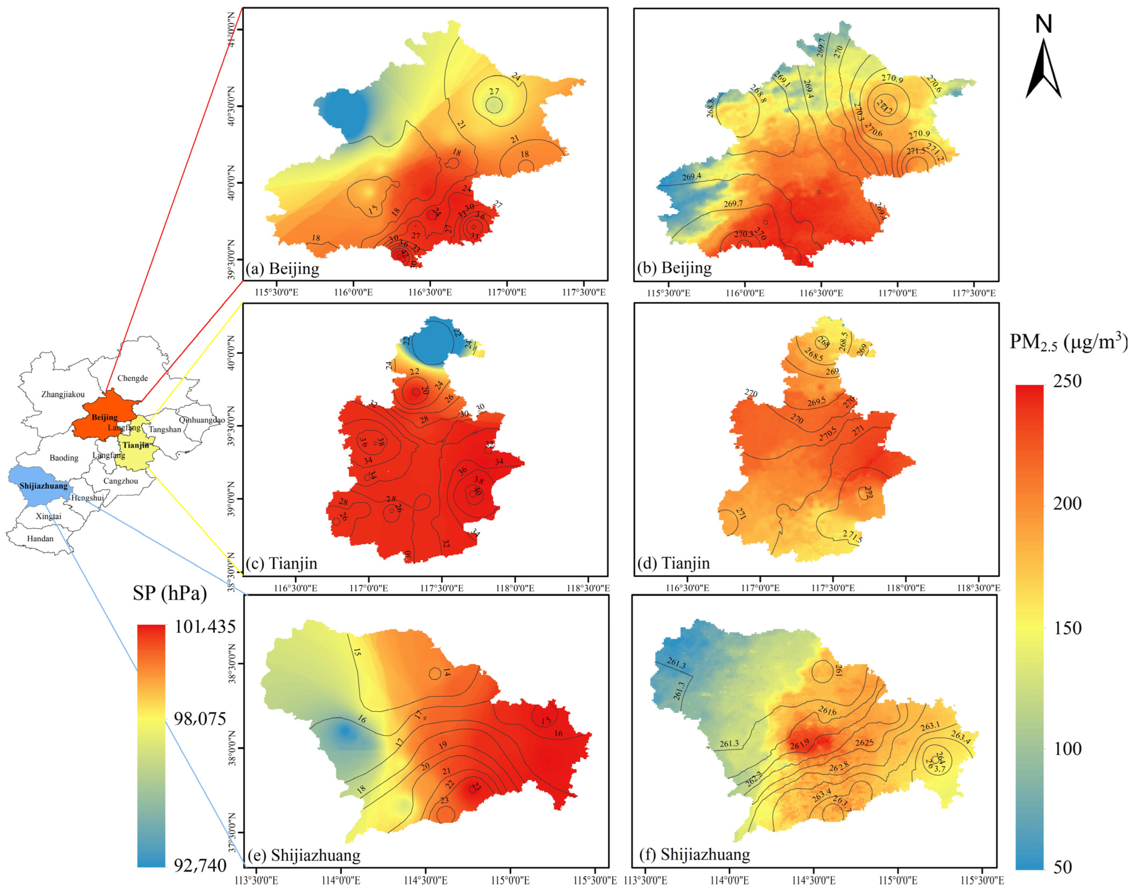It can be concluded from Table 4 that the model effect after adding wavelet decomposition was significantly better than without it, which is due to the fact that adding wavelet decomposition can make full use of the high-frequency and low-frequency components of the PM_2.5 data. We used a total of seven meteorological elements for model training, and the results showed that the boundary layer height was the most important meteorological predictor, followed by surface pressure and temperature. By adding meteorological elements as auxiliary parameters for model construction, it was shown that auxiliary data such as surface pressure and temperature play an important role in PM_2.5 estimations.

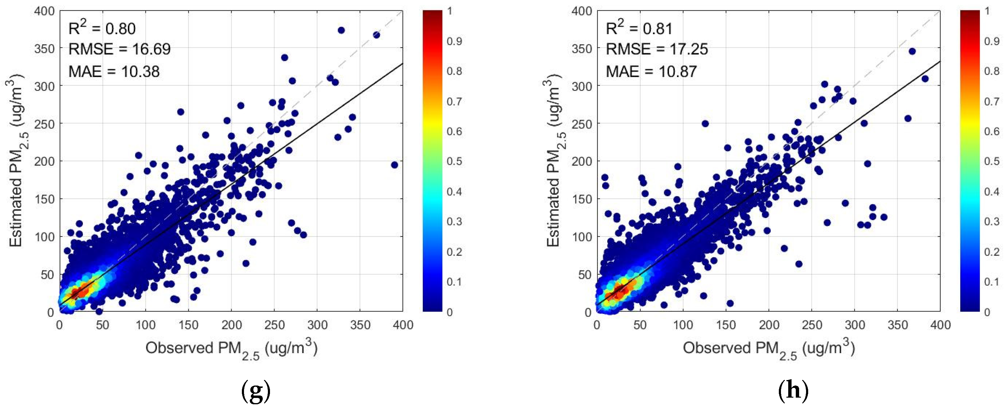
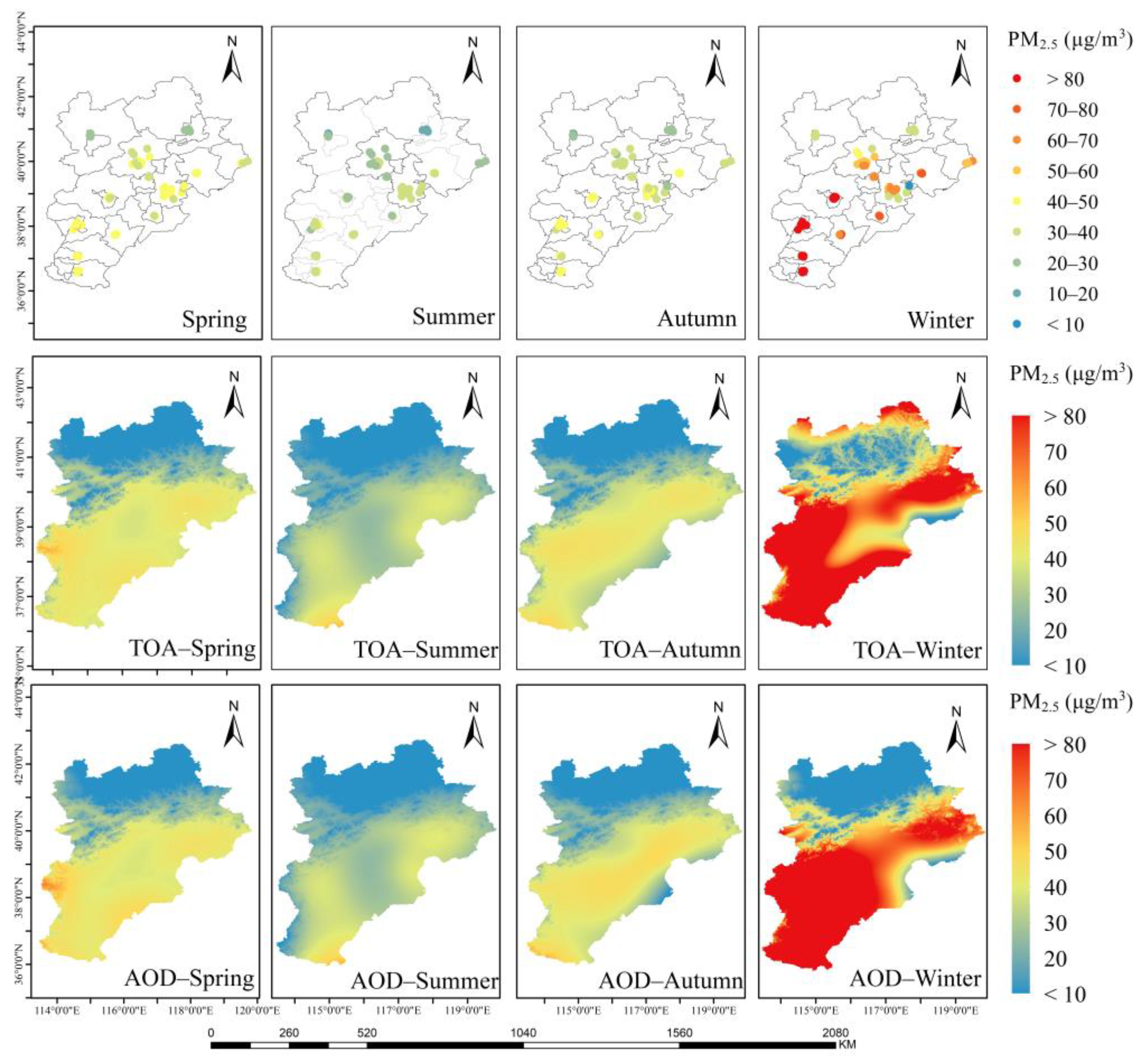
Satellite data have now been widely used to estimate ground-based PM_2.5 concentrations using various models to construct the relationship between satellite data and PM_2.5. However, it can be seen from Figure 7 that the estimation of PM_2.5 concentrations using AOD and TOAR, respectively, had the most significant error in winter, and it can be seen from Figure 8 that during the winter period, the R² of the prediction performance using TOAR improved by 0.02, and the RMSE and MAE decreased by 2.97 and 2.54, respectively, compared with that using AOD. This is due to the limited coverage of AOD and the vulnerability to external conditions resulting in missing data. The satellite TOAR can effectively compensate for the lack of spatial coverage of AOD and the limitation of the inversion method by replacing AOD for PM_2.5 concentration estimation. Therefore, we selected TOAR as the satellite data for estimating PM_2.5.

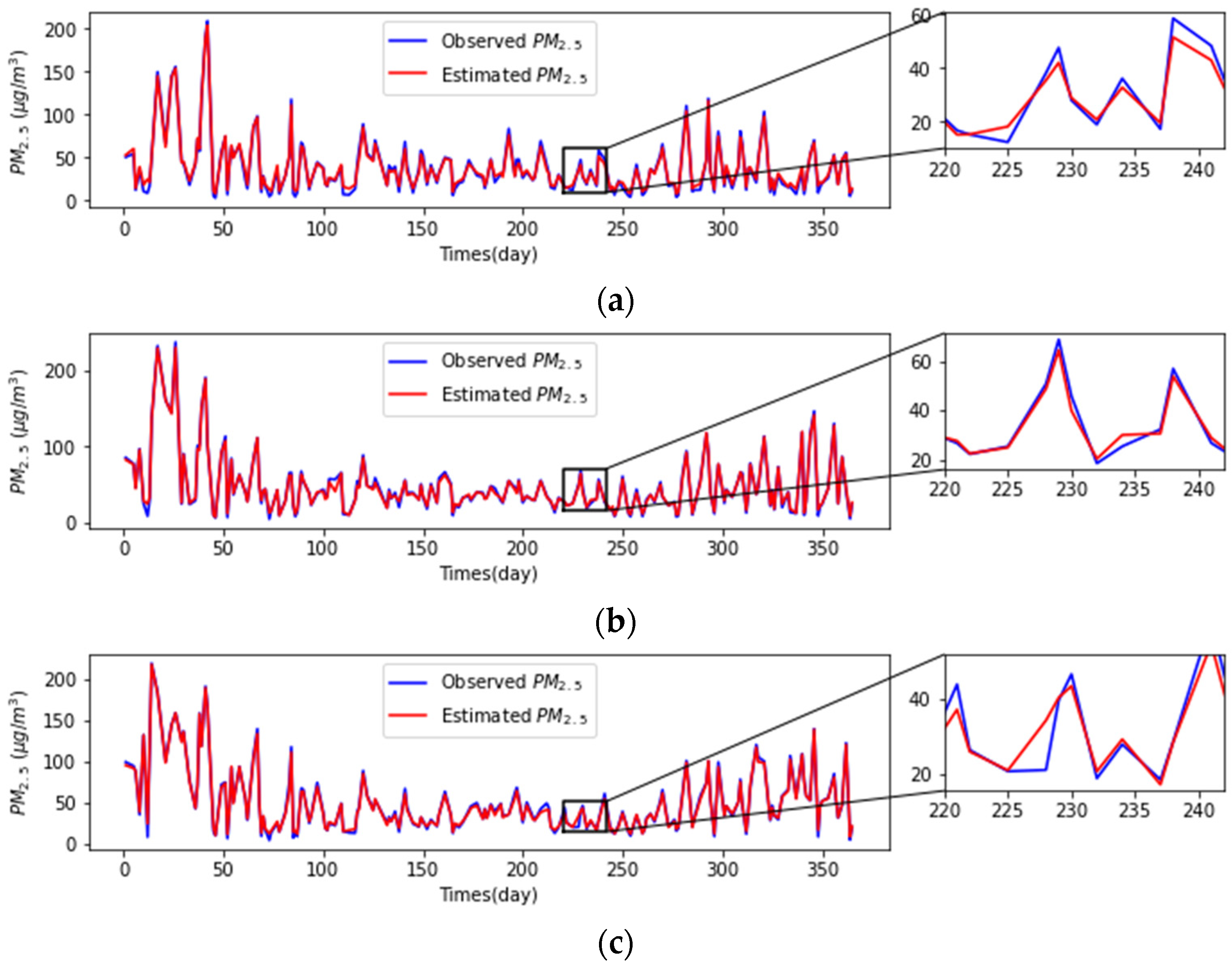
Based on the results of the model, we analyzed the spatial and temporal characteristics of PM_2.5 concentrations in the Beijing–Tianjin–Hebei region by season, with the lightest pollution in summer, the most serious pollution in winter, and spring and autumn in between; meanwhile, three more seriously polluted areas (Beijing, Tianjin, and Shijiazhuang) were selected to analyze the trends of daily PM_2.5 concentrations over one year, and they were further studied to conclude that PM_2.5 concentrations and meteorological elements are highly correlated. Compared with previous studies, the proposed hybrid learning model outperformed most advanced statistical models and machine learning models in terms of prediction performance, running speed, and memory consumption. Therefore, the hybrid learning model using TOAR and correlation variables can be a good alternative to AOD for PM_2.5 high-precision predictions, which is useful for pollution prevention and control in the Beijing–Tianjin–Hebei region.

At the same time, this study also had certain limitations: (a) the research used the data of state-controlled sites, which are mainly distributed in the central areas of the city or in the more polluted areas; so, the model validation was also based on city center sites. In future research, the provincial-controlled sites and national-controlled sites will be used as research data to improve the regional representativeness of the sample and the generalization ability of the model; (b) PM_2.5 concentrations are affected by many factors, such as population density, traffic flow, and Normalized Difference Vegetation Index (NDVI), etc.; these influencing factors were lacking in this study. In future research on PM_2.5 concentration estimation, data from more sources will be collected, and various factors will be comprehensively considered.

5. Conclusions

Here, we proposed a hybrid learning model that used satellite TOAR, meteorological elements, and elevation data to predict daily PM_2.5 concentrations in the Beijing–Tianjin–Hebei region. After experimental verification, we drew the following conclusions.

(1)

Using satellite TOAR instead of AOD to directly estimate PM_2.5 concentrations enables a higher prediction accuracy to be obtained.

(2)

The hybrid learning model proposed in this study had high prediction accuracy and universality and was suitable for near-ground PM_2.5 concentrations estimation: adding wavelet decomposition to the model extracted periodic features and random features of the original time series; using the fusion of two machine learning models not only took advantage of the minimum number of trees established by the random forest model but also took into account that the LightGBM model required less running memory and running time.

To summarize, satellite TOAR replaced AOD to estimate ground PM_2.5 concentrations, avoided the intermediate process of AOD inversion, and effectively made up for the low space–time coverage of AOD. Hybrid learning models can handle nonlinear relationships between factors well, outperforming most advanced statistical models and machine learning methods. In future research, more parameters closely related to PM_2.5 will be considered to further improve the performance of the model, and the model can also be applied to the concentration estimation of other air pollutants, such as SO₂, NO₂, etc.

References

1. Yang, L.; Xu, H.; Jin, Z. Estimating Ground-Level PM2.5 over a Coastal Region of China Using Satellite AOD and a Combined Model. J. Clean. Prod. 2019, 227, 472–482. [Google Scholar] [CrossRef]
2. Fan, H.; Zhao, C.; Yang, Y. A Comprehensive Analysis of the Spatio-Temporal Variation of Urban Air Pollution in China during 2014–2018. Atmos. Environ. 2020, 220, 117066. [Google Scholar] [CrossRef]
3. Song, Y.; Huang, B.; He, Q.; Chen, B.; Wei, J.; Mahmood, R. Dynamic Assessment of PM2.5 Exposure and Health Risk Using Remote Sensing and Geo-Spatial Big Data. Environ. Pollut. 2019, 253, 288–296. [Google Scholar] [CrossRef] [PubMed]
4. Ebenstein, A.; Fan, M.; Greenstone, M.; He, G.; Zhou, M. New Evidence on the Impact of Sustained Exposure to Air Pollution on Life Expectancy from China’s Huai River Policy. Proc. Natl. Acad. Sci. USA 2017, 114, 10384–10389. [Google Scholar] [CrossRef] [PubMed] [Green Version]
5. Chen, B.-Y.; Chen, C.-H.; Chuang, Y.-C.; Wu, Y.-H.; Pan, S.-C.; Guo, Y.L. Changes in the Relationship between Ambient Fine Particle Concentrations and Childhood Lung Function over 5 Years. Environ. Res. 2019, 179, 108809. [Google Scholar] [CrossRef]
6. Wu, W.; Zhang, M.; Ding, Y. Exploring the Effect of Economic and Environment Factors on PM2.5 Concentration: A Case Study of the Beijing-Tianjin-Hebei Region. J. Environ. Manag. 2020, 268, 110703. [Google Scholar] [CrossRef]
7. Bi, W.; Chen, K.; Xiao, Z.; Tang, M.; Zheng, N.; Yang, N.; Gao, J.; Li, Y.; Kong, J.; Xu, H. Health Benefit Assessment of China’s National Action Plan on Air Pollution in the Beijing-Tianjin-Hebei Area. Aerosol Air Qual. Res. 2019, 19, 383–389. [Google Scholar] [CrossRef]
8. Ho, C.-C.; Chen, L.-J.; Hwang, J.-S. Estimating Ground-Level PM2.5 Levels in Taiwan Using Data from Air Quality Monitoring Stations and High Coverage of Microsensors. Environ. Pollut. 2020, 264, 114810. [Google Scholar] [CrossRef]
9. Wu, J.; Li, T.; Zhang, C.; Cheng, Q.; Shen, H. Hourly PM 2.5 Concentration Monitoring With Spatiotemporal Continuity by the Fusion of Satellite and Station Observations. IEEE J. Sel. Top. Appl. Earth Obs. Remote Sens. 2021, 14, 8019–8032. [Google Scholar] [CrossRef]
10. Dong, L.; Li, S.; Yang, J.; Shi, W.; Zhang, L. Investigating the Performance of Satellite-Based Models in Estimating the Surface PM2.5 over China. Chemosphere 2020, 256, 127051. [Google Scholar] [CrossRef]
11. Ma, Z.; Hu, X.; Huang, L.; Bi, J.; Liu, Y. Estimating Ground-Level PM2.5 in China Using Satellite Remote Sensing. Environ. Sci. Technol. 2014, 48, 7436–7444. [Google Scholar] [CrossRef]
12. Li, Y.; Yuan, S.; Fan, S.; Song, Y.; Wang, Z.; Yu, Z.; Yu, Q.; Liu, Y. Satellite Remote Sensing for Estimating PM2.5 and Its Components. Curr. Pollut. Rep. 2021, 7, 72–87. [Google Scholar] [CrossRef]
13. He, Q.; Wang, M.; Yim, S.H.L. The Spatiotemporal Relationship between PM2.5 and Aerosol Optical Depth in China: Influencing Factors and Implications for Satellite PM2.5 Estimations Using MAIAC Aerosol Optical Depth. Atmos. Chem. Phys. 2021, 21, 18375–18391. [Google Scholar] [CrossRef]
14. Zhang, T.; Zhu, Z.; Gong, W.; Zhu, Z.; Sun, K.; Wang, L.; Huang, Y.; Mao, F.; Shen, H.; Li, Z.; et al. Estimation of Ultrahigh Resolution PM2.5 Concentrations in Urban Areas Using 160 m Gaofen-1 AOD Retrievals. Remote Sens. Environ. 2018, 216, 91–104. [Google Scholar] [CrossRef]
15. Xue, Y.; Li, Y.; Guang, J.; Tugui, A.; She, L.; Qin, K.; Fan, C.; Che, Y.; Xie, Y.; Wen, Y.; et al. Hourly PM2.5 Estimation over Central and Eastern China Based on Himawari-8 Data. Remote Sens. 2020, 12, 855. [Google Scholar] [CrossRef] [Green Version]
16. Zeng, Q.; Chen, L.; Zhu, H.; Wang, Z.; Wang, X.; Zhang, L.; Gu, T.; Zhu, G.; Zhang, Y. Satellite-Based Estimation of Hourly PM2.5 Concentrations Using a Vertical-Humidity Correction Method from Himawari-AOD in Hebei. Sensors 2018, 18, 3456. [Google Scholar] [CrossRef] [Green Version]
17. Tang, Y.; Deng, R.; Li, J.; Liang, Y.; Xiong, L.; Liu, Y.; Zhang, R.; Hua, Z. Estimation of Ultrahigh Resolution PM2.5 Mass Concentrations Based on Mie Scattering Theory by Using Landsat8 OLI Images over Pearl River Delta. Remote Sens. 2021, 13, 2463. [Google Scholar] [CrossRef]
18. Wang, W.; Mao, F.; Du, L.; Pan, Z.; Gong, W.; Fang, S. Deriving Hourly PM2.5 Concentrations from Himawari-8 AODs over Beijing–Tianjin–Hebei in China. Remote Sens. 2017, 9, 858. [Google Scholar] [CrossRef] [Green Version]
19. Mirzaei, M.; Amanollahi, J.; Tzanis, C.G. Evaluation of Linear, Nonlinear, and Hybrid Models for Predicting PM2.5 Based on a GTWR Model and MODIS AOD Data. Air Qual. Atmos. Health 2019, 12, 1215–1224. [Google Scholar] [CrossRef]
20. He, Q.; Huang, B. Satellite-Based High-Resolution PM2.5 Estimation over the Beijing-Tianjin-Hebei Region of China Using an Improved Geographically and Temporally Weighted Regression Model. Environ. Pollut. 2018, 236, 1027–1037. [Google Scholar] [CrossRef] [PubMed]
21. Chu, H.-J.; Bilal, M. PM2.5 Mapping Using Integrated Geographically Temporally Weighted Regression (GTWR) and Random Sample Consensus (RANSAC) Models. Environ. Sci. Pollut. Res. 2019, 26, 1902–1910. [Google Scholar] [CrossRef] [PubMed]
22. Yan, X.; Zang, Z.; Jiang, Y.; Shi, W.; Guo, Y.; Li, D.; Zhao, C.; Husi, L. A Spatial-Temporal Interpretable Deep Learning Model for Improving Interpretability and Predictive Accuracy of Satellite-Based PM2.5. Environ. Pollut. 2021, 273, 116459. [Google Scholar] [CrossRef] [PubMed]
23. Li, X.; Zhang, X. Predicting Ground-Level PM2.5 Concentrations in the Beijing-Tianjin-Hebei Region: A Hybrid Remote Sensing and Machine Learning Approach. Environ. Pollut. 2019, 249, 735–749. [Google Scholar] [CrossRef] [PubMed] [Green Version]
24. Wei, J.; Li, Z.; Pinker, R.T.; Wang, J.; Sun, L.; Xue, W.; Li, R.; Cribb, M. Himawari-8-Derived Diurnal Variations in Ground-Level PM2.5 Pollution across China Using the Fast Space-Time Light Gradient Boosting Machine (LightGBM). Atmos. Chem. Phys. 2021, 21, 7863–7880. [Google Scholar] [CrossRef]
25. Kim, S.-M.; Koo, J.-H.; Lee, H.; Mok, J.; Choi, M.; Go, S.; Lee, S.; Cho, Y.; Hong, J.; Seo, S.; et al. Comparison of PM2.5 in Seoul, Korea Estimated from the Various Ground-Based and Satellite AOD. Appl. Sci. 2021, 11, 10755. [Google Scholar] [CrossRef]
26. Pu, Q.; Yoo, E.-H. Ground PM2.5 Prediction Using Imputed MAIAC AOD with Uncertainty Quantification. Environ. Pollut. 2021, 274, 116574. [Google Scholar] [CrossRef] [PubMed]
27. Shen, H.; Li, T.; Yuan, Q.; Zhang, L. Estimating Regional Ground-Level PM2.5 Directly From Satellite Top-of-Atmosphere Reflectance Using Deep Belief Networks. J. Geophys. Res. Atmos. 2018, 123, 13,875–13,886. [Google Scholar] [CrossRef] [Green Version]
28. Bai, H.; Zheng, Z.; Zhang, Y.; Huang, H.; Wang, L. Comparison of Satellite-Based PM2.5 Estimation from Aerosol Optical Depth and Top-of-Atmosphere Reflectance. Aerosol Air Qual. Res. 2021, 21, 200257. [Google Scholar] [CrossRef]
29. Yang, L.; Xu, H.; Yu, S. Estimating PM2.5 Concentrations in Yangtze River Delta Region of China Using Random Forest Model and the Top-of-Atmosphere Reflectance. J. Environ. Manag. 2020, 272, 111061. [Google Scholar] [CrossRef]
30. Yin, J.; Mao, F.; Zang, L.; Chen, J.; Lu, X.; Hong, J. Retrieving PM2.5 with High Spatio-Temporal Coverage by TOA Reflectance of Himawari-8. Atmos. Pollut. Res. 2021, 12, 14–20. [Google Scholar] [CrossRef]
31. Zhao, G.; Huang, G.; He, H.; He, H.; Ren, J. Regional Spatiotemporal Collaborative Prediction Model for Air Quality. IEEE Access 2019, 7, 134903–134919. [Google Scholar] [CrossRef]
32. Ding, Y.; Chen, Z.; Lu, W.; Wang, X. A CatBoost Approach with Wavelet Decomposition to Improve Satellite-Derived High-Resolution PM2.5 Estimates in Beijing-Tianjin-Hebei. Atmos. Environ. 2021, 249, 118212. [Google Scholar] [CrossRef]
33. Wang, J.; He, L.; Lu, X.; Zhou, L.; Tang, H.; Yan, Y.; Ma, W. A Full-Coverage Estimation of PM2.5 Concentrations Using a Hybrid XGBoost-WD Model and WRF-Simulated Meteorological Fields in the Yangtze River Delta Urban Agglomeration, China. Environ. Res. 2022, 203, 111799. [Google Scholar] [CrossRef]
34. Song, Z.; Chen, B.; Huang, Y.; Dong, L.; Yang, T. Estimation of PM2.5 Concentration in China Using Linear Hybrid Machine Learning Model. Atmos. Meas. Tech. 2021, 14, 5333–5347. [Google Scholar] [CrossRef]
35. Liu, J.; Weng, F.; Li, Z. Satellite-Based PM2.5 Estimation Directly from Reflectance at the Top of the Atmosphere Using a Machine Learning Algorithm. Atmos. Environ. 2019, 208, 113–122. [Google Scholar] [CrossRef]
36. Mehdizadeh, S.; Ahmadi, F.; Danandeh Mehr, A.; Safari, M.J.S. Drought Modeling Using Classic Time Series and Hybrid Wavelet-Gene Expression Programming Models. J. Hydrol. 2020, 587, 125017. [Google Scholar] [CrossRef]
37. Khosravi, I.; Alavipanah, S.K. A Random Forest-Based Framework for Crop Mapping Using Temporal, Spectral, Textural and Polarimetric Observations. Int. J. Remote Sens. 2019, 40, 7221–7251. [Google Scholar] [CrossRef]
38. Chen, C.; Zhang, Q.; Ma, Q.; Yu, B. LightGBM-PPI: Predicting Protein-Protein Interactions through LightGBM with Multi-Information Fusion. Chemom. Intell. Lab. Syst. 2019, 191, 54–64. [Google Scholar] [CrossRef]
39. Zhong, J.; Zhang, X.; Gui, K.; Wang, Y.; Che, H.; Shen, X.; Zhang, L.; Zhang, Y.; Sun, J.; Zhang, W. Robust Prediction of Hourly PM2.5 from Meteorological Data Using LightGBM. Natl. Sci. Rev. 2021, 8, nwaa307. [Google Scholar] [CrossRef]
40. Liang, W.; Luo, S.; Zhao, G.; Wu, H. Predicting Hard Rock Pillar Stability Using GBDT, XGBoost, and LightGBM Algorithms. Mathematics 2020, 8, 765. [Google Scholar] [CrossRef]
41. Paul, D.; Goswami, A.K.; Chetri, R.L.; Roy, R.; Sen, P. Bayesian Optimization-Based Gradient Boosting Method of Fault Detection in Oil-Immersed Transformer and Reactors. IEEE Trans. Ind. Appl. 2022, 58, 1910–1919. [Google Scholar] [CrossRef]
42. Hua, Z.; Sun, W.; Yang, G.; Du, Q. A Full-Coverage Daily Average PM2.5 Retrieval Method with Two-Stage IVW Fused MODIS C6 AOD and Two-Stage GAM Model. Remote Sens. 2019, 11, 1558. [Google Scholar] [CrossRef] [Green Version]
43. He, Q.; Huang, B. Satellite-Based Mapping of Daily High-Resolution Ground PM2.5 in China via Space-Time Regression Modeling. Remote Sens. Environ. 2018, 206, 72–83. [Google Scholar] [CrossRef]
44. Xue, W.; Zhang, J.; Zhong, C.; Li, X.; Wei, J. Spatiotemporal PM2.5 Variations and Its Response to the Industrial Structure from 2000 to 2018 in the Beijing-Tianjin-Hebei Region. J. Clean. Prod. 2021, 279, 123742. [Google Scholar] [CrossRef]
45. Wei, J.; Huang, W.; Li, Z.; Xue, W.; Peng, Y.; Sun, L.; Cribb, M. Estimating 1-Km-Resolution PM2.5 Concentrations across China Using the Space-Time Random Forest Approach. Remote Sens. Environ. 2019, 231, 111221. [Google Scholar] [CrossRef]
46. Xiao, Q.; Wang, Y.; Chang, H.H.; Meng, X.; Geng, G.; Lyapustin, A.; Liu, Y. Full-Coverage High-Resolution Daily PM2.5 Estimation Using MAIAC AOD in the Yangtze River Delta of China. Remote Sens. Environ. 2017, 199, 437–446. [Google Scholar] [CrossRef]
Figure 1. Elevation map of Beijing–Tianjin–Hebei region.
Remotesensing 14 02714 g001
Figure 2. Technology Roadmap.
Remotesensing 14 02714 g002
Figure 3. Graph of wavelet decomposition results.
Remotesensing 14 02714 g003
Figure 4. Bagging Algorithm Flowchart.
Remotesensing 14 02714 g004
Figure 5. Flowchart of the Bayesian Optimization Algorithm.
Remotesensing 14 02714 g005
Figure 6. Scatter plots of the model prediction results with different input variables versus the actual PM2.5 values. TOAR-based on the left and AOD-based on the right. Wavelet decomposition is added to (a,b,e,f) and not added to (c,d,g,h); meteorological elements are added to (ad) and not added to (eh). The dashed line is the 1:1 line, and the solid line is the fitted line.
Remotesensing 14 02714 g006aRemotesensing 14 02714 g006b
Figure 7. Seasonal average distribution of PM2.5 concentrations in the Beijing–Tianjin–Hebei region.
Remotesensing 14 02714 g007
Figure 8. Density scatter plots of PM2.5 concentrations by seasonal cross-validation results in 2020. TOAR-based on the left and AOD-based on the right, (a,b) spring, (c,d) summer, (e,f) autumn, and (g,h) winter; the dashed line is the 1:1 line, and the solid line is the fitted line.
Remotesensing 14 02714 g008
Figure 9. Time series of observed (blue) and estimated (red) daily PM2.5 concentrations in 2020. (a) Beijing, (b) Tianjin, and (c) Shijiazhuang.
Remotesensing 14 02714 g009
Figure 10. Pollution in Beijing (12 February 2020), Tianjin (27 January 2020), and Shijiazhuang (15 January 2020). (a,c,e) Depict the boundary layer height and surface pressure in the three regions. The black curve represents the boundary layer height contour (unit: m), and the background represents the surface pressure. (b,d,f) Depict the temperature and PM2.5 concentrations estimated by the hybrid model for the three regions, with the black curves representing the temperature contours (unit: K), and the background represents the PM2.5 concentrations.
Remotesensing 14 02714 g010