Estimation of Downwelling Surface Longwave Radiation with the Combination of Parameterization and Artificial Neural Network from Remotely Sensed Data for Cloudy Sky Conditions

Abstract

This work proposes a new method for estimating downwelling surface longwave radiation (DSLR) under cloudy-sky conditions based on a parameterization method and a genetic algorithm–artificial neural network (GA-ANN) algorithm. The new method establishes a GA-ANN model based on simulated data, and then combines MODIS satellite data and ERA5 reanalysis data to estimate the DSLR. According to the validation results of the field sites, the bias and RMSE are –9.18 and 34.88 W/m², respectively. Compared with the existing research, the new method can achieve reasonable accuracy. Parameter analysis using independently simulated data shows that the near-surface air temperature ($T_a$) and cloud base height (CBH) have an important influence on DSLR estimation under cloudy-sky conditions. With an increase in CBH, DSLR gradually decreases; however, with an increase in $T_a$, DSLR shows a trend of gradual increase. When estimating DSLR under cloudy-sky conditions, under the influence of clouds, except for cirrus, the change in DSLRs with CBH and $T_a$ is greater than 20 W/m².

1. Introduction

The downwelling surface longwave radiation (DSLR) is an important component of surface net longwave radiation, which is significant for surface radiation balance and is mainly affected by factors such as atmospheric temperature, water vapor content (WVC), and clouds. The effect of clouds on longwave radiation is mainly to absorb longwave radiation from the atmosphere and the surface; at the same time, as a radiator, it has an impact on the atmosphere. At present, there are two main methods for estimating the DSLR under cloudy-sky conditions: one is an empirical algorithm that modifies or adds cloud parameters based on clear-sky conditions, and the other establishes a parameterization algorithm based on different cloud characteristics, such as cloud base temperature or cloud top temperature.

For empirical algorithms, DSLR estimation under cloudy-sky conditions is mainly used as the cloud fraction to correct the estimation method under clear-sky conditions. Studies [1,2,3,4] estimated the cloud fraction using the ratio of the observed solar radiation to the simulated clear-sky solar radiation. Rooney [5] proposed obtaining the estimated cloud fraction from the output data of the laser cloud-based recorder. Zhong et al. [6] adjusted the parameters of the model proposed by Crawford and Duchon [3] and obtained a DSLR model under cloudy-sky conditions by considering the influence of clouds on air emissivity. Cheng et al. [7] evaluated seven widely used DSLR algorithms under all-sky conditions using ground measurement data collected from 44 globally distributed flux measurement sites. Additionally, Cheng et al. [7] introduced the Bayesian model averaging method to integrate multiple estimation formulas and obtain the estimation of DSLR under cloudy-sky conditions. Liu et al. [8] used longwave radiation measurement data from three observation sites on the Qinghai-Tibet Plateau to make parameter adjustments to the four commonly used parameterization schemes under cloudy-sky conditions. After local calibration of the parameters, it was found that combining the clear-sky parameterization of Dilley and O’Brien [9] with the cloud correction scheme of Jacobs [10] achieves the best result. In addition, Liu et al. [8] found that the cloud base height (CBH) has a significant impact on DSLR estimation under cloudy-sky conditions, resulting in an improved parameterization scheme to estimate the DSLR based on the CBH.

For parameterization algorithms, many scholars have considered the influence of cloud base temperature and estimated DSLR under cloudy-sky conditions based on a single-layer cloud model. Wang et al. [11] fused Moderate-resolution Imaging Spectroradiometer (MODIS) atmospheric temperature profile data under clear skies with the Atmospheric Infrared Sounder (AIRS)/the Advanced Microwave Sounding Unit (AMSU) temperature profile data under cloudy skies to obtain a high spatial resolution sub-cloud atmospheric profile. The cloud base temperature was obtained using this fused temperature profile data. Yang and Cheng [12] used the constructed cloud attribute database to adjust the coefficients of the Clouds and Earth’s Radiant Energy Systems (CERES) cloud geometric thickness model, calculated the CBH based on cloud top height and geometric thickness, and then used the temperature profile of the reanalysis data to obtain the cloud base temperature. Ahn et al. [13,14] developed an algorithm to calculate the DSLR under all-sky conditions using cloud base temperature and precipitable water between clouds and ground. Some scholars use cloud top temperature instead of cloud base temperature to estimate DSLR because cloud base temperatures obtained from passive remote sensing data have greater uncertainty. Wang et al. [15] used cloud top temperature to replace cloud base temperature, combined with land surface temperature and atmospheric water vapor content under clear-sky conditions, and used a nonlinear parametric model to estimate the DSLR.

Compared with DSLR estimation under clear-sky conditions, there is a large uncertainty in DSLR estimation under cloudy-sky conditions, regardless of whether an empirical algorithm or parameterized algorithm was used. The empirical algorithm under cloudy-sky conditions was generated using a specific dataset under a specific underlying surface condition. Most of the empirical algorithms under cloudy-sky conditions use CF to correct the algorithm under clear-sky conditions, and do not fully consider the influence of CBH on DSLR estimation. The parameterization method based on the cloud base temperature or cloud top temperature has a strong universality and can obtain better results across applications. However, the CBH used to determine the cloud base temperature has mostly been estimated using different empirical algorithms, and its estimation methods are not mature. At present, relatively mature CBH products have been developed based on ERA5 reanalysis data, but few scholars have applied it to DSLR estimation. In this study, a new method was developed to estimate the DSLR under cloudy-sky conditions by directly using the CBH from ERA5 reanalysis data and combining the radiance at the top of the atmosphere (TOA), WVC, and $T_a$ data. The remainder of this article is organized as follows: Section 2 describes the datasets used in this study, Section 3 presents the GA-ANN model construction and DSLR estimation method under cloudy-sky conditions, Section 4 presents the results of the GA-ANN algorithm and a sensitivity analysis, Section 5 provides validation using in situ measurements and comparisons with existing methods, Section 6 presents the discussion, and conclusions are presented in Section 7.

2. Data

2.1. MODIS Satellite Data

MODIS is a medium-resolution passive imaging spectroradiometer that is carried on the Terra and Aqua platforms of American polar-orbiting satellites. It collects a total of 36 groups of wavelengths, or bands, and the spectral coverage ranges from 0.405 to 14.385 μm. These data have a very high signal-to-noise ratio. In the scientific fields of ocean, land, and atmosphere, there have been many applied studies on MODIS, and a variety of products of different levels have been produced to meet the needs of Earth science research (http://modis.gsfc.nasa.gov/data/dataprod/index.php; accessed on 30 May 2022). Terra-MODIS products from 2010, 2017, and 2018 were employed in this study. They are MOD021KM, MOD03, MOD05, and MOD35 (

Table 1. Satellite data and reanalysis data used in this study.

Data Sources	Product	Resolution	Parameters
MODIS	MOD021KM	1 km	Radiance of bands 28, 29, 31, 33, 34, 36
	MOD03	1 km	Latitude, Longitude
	MOD05	1 km	WVC
	MOD35	1 km	Cloud mask
ERA5		0.25° × 0.25°	Cloud base height
		0.25° × 0.25°	Total cloud cover
		0.25° × 0.25°	2 m air temperature
		0.25° × 0.25°	2 m dew point temperature
		0.25° × 0.25°	Cloud base temperature

). MOD021KM products are level 1 products with radiation correction and contain reflectance and radiance data at the TOA [16]. The spatial resolution of channels 1–2 is 250 m, channels 3–7 is 500 m, and channels 8–36 is 1 km. This study mainly used TOA radiance of bands 28, 29, 31, 33, 34, and 36. MOD03 products are level 1 products used for data geolocation. It provides information such as the geographic coordinates of each pixel with a resolution of 1 km, including latitude, longitude, ground elevation, satellite view zenith angle (VZA), and sea and land masks [17]. This study uses latitude and longitude data, as well as satellite VZA data. MOD05 is a level 2 product of the total precipitable water vapor. Atmospheric water vapor content data were used in this study. MOD35 is a cloud mask product used in this study to distinguish cloud pixels.

2.2. Reanalysis Data

ERA5 is a fifth-generation reanalysis product launched by the European Center for Medium-Term Weather Forecasts (ECWMF) after ERA-Interim. It provides a large number of ocean climate and hourly climate variables with a spatial resolution of 0.25° × 0.25°, the vertical resolution ranges from 1000 to 1 hPa, a total of 37 layers, and a time resolution of 1 h. This study employed the CBH, total cloud cover, 2 m air temperature, and 2 m dew point temperature from ERA5 hourly data on single levels (Table 1). In addition, this study employed ERA5 hourly data on pressure levels to obtain the cloud base temperature at the CBH location.

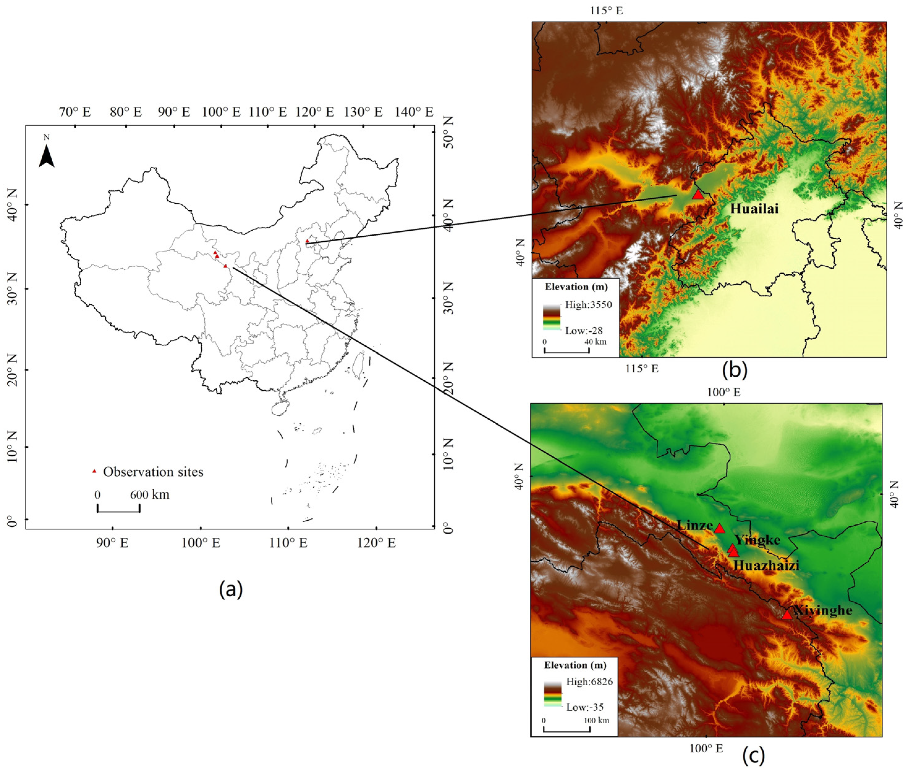
2.3. Site Observations

This study selected three observation network sites to verify the accuracy of the estimated DSLR: the Chinese Watershed Allied Telemetry Experimental Research (WATER) in the Heihe River Basin [18,19,20,21], the Qilian Mountains integrated observatory network in the Cold and Arid Research Network of Lanzhou University (CARN), and the multi-scale surface flux and meteorological element observation dataset in the Hai River Basin (HAIHE) [22,23]. The Heihe River Basin and Qilian Mountain Basin are located in arid and semi-arid regions of Northwest China. The underlying surface includes alpine snow, ice belts, forest grassland belts, plain oasis belts, gobi desert belts, and other landscape types. The Haihe River Basin is located on the North China Plain. Within the territory, climatic conditions are relatively favorable, and the types of surface coverage are more complicated. Based on the data availability and quality control documents of the observation sites, the verification sites selected in this study included the Yingke Observation Site and the Huazhaizi Observation Site in the middle reaches of the Heihe River basin, the Huailai site in the Haihe River basin, and the Xiyinghe Observation Site and Linze Observation Site of the Qilian Mountains Basin (Figure 1). These sites are equipped with automatic weather stations and four-component radiation meters that can continuously obtain flux observation data. Measurement data included total solar radiation, reflected radiation, downwelling longwave radiation, and upwelling longwave radiation. The time resolution was 10 min.

Table 2. Descriptions of site conditions.

Site Name	Lat and Lon (Deg)	Land Cover	Elevation (m)	Temporal Period
Yingke	38.85, 100.4167	Cropland	1519	2010.01.01–2010.12.31
Huazhaizi	38.7667, 100.45	Desert	1731	2010.01.01–2010.12.31
Linze	39.238, 100.062	Cropland	1402	2018.01.01–2018.12.31
Xiyinghe	37.561, 101.855	Alpine grassland	3616	2018.01.01–2018.12.31
Huailai	40.3574, 115.7928	Cropland	480	2017.01.01–2017.12.31

lists the latitude, longitude, surface type, elevation, and verification time range for each site.

2.4. Simulated Data

The atmospheric radiation transmission model, MODTRAN 5 [24], was used to simulate DSLR estimation under cloudy-sky conditions. To cover all atmosphere and surface conditions, the sounding database used in the simulation was the latest version of the Thermodynamic Initial Guess Retrieval, i.e., TIGR2002, which was constructed by the Laboratoire de Meteorologie Dynamique (LMD) (https://ara.lmd.polytechnique.fr/index.php?page=tigr; accessed on 30 May 2022). This database uses complex statistical methods to select 2311 atmospheric profiles from different periods and global statistical samples from polar to tropical regions to provide as many global atmospheric conditions as possible. Each atmospheric profile represents different atmospheric conditions, including air temperature, air pressure, WVC, and ozone content. The purpose of this study is to establish a DSLR estimation method for cloudy-sky conditions. Then, the TIGR2002 profiles with relative humidity (RH) greater than 90% were identified as cloudy-sky profiles, while the rest were identified as clear-sky profiles. According to the judgment of the cloudy sky, the atmospheric profile affected by clouds was screened out, and 1365 atmospheric profiles under cloudy-sky conditions and 946 atmospheric profiles under clear-sky conditions were obtained, respectively. Eight feature types were chosen to represent as many different underlying surface types as possible in the MODTRAN 5 simulations. These features include evergreen broadleaf forest, grassland, wetland, sandy loam, barren desert, urban, ocean water, and fresh snow. Considering the angular dependence of the TOA radiance and maximum observed zenith angle of MODIS (less than 65° from the lowest point), different observed zenith angles from 0° to 60° were used to calculate the TOA radiance and DSLR of the MODIS infrared channel in the MODTRAN simulation. To set the cloudy-sky parameters, seven types of clouds provided by MODTRAN were selected for the simulation, including cumulus, altostratus, stratus, stratus/stratocumulus, nimbostratus, standard cirrus, and subvisual cirrus. The CBH was set to the default CBH for each cloud type in MODTRAN. Finally, set variables were input into MODTRAN to obtain the simulation value of the DSLR under cloudy-sky conditions. A total of 458,640 samples were prepared for the MODTRAN simulation code, and the DSLR, TOA radiance, CBH, $T_a$, VZA, and WVC were used to establish the machine learning algorithm under cloudy-sky conditions. When the simulation is carried out under clear-sky conditions, the input parameters are set to be the same as those under cloudy-sky conditions, except that the information related to cloud parameters is not set, while the DSLR, TOA radiance, $T_a$, VZA, and WVC were used to establish the machine learning algorithm.

3. Methodology

3.1. Estimating DSLR under Cloudy-Sky Conditions

DSLR under cloudy-sky conditions can be expressed as:

$$DSLR=DSL{R}_{clear}\times 1-CF+DSL{R}_{cloudy}\times CF$$

(1)

where $DSL{R}_{clear}$ represents downwelling longwave radiation under clear-sky conditions, $DSL{R}_{cloudy}$ represents downwelling longwave radiation under fully cloudy-sky conditions, and CF represents fractional cloud cover. The first term on the right side represents the radiation from the cloudless coverage area in the pixel, and the second term represents the radiation from the cloud coverage area in the pixel.

Based on the cloud fraction, the DSLR estimation under cloudy-sky conditions was divided into partially and fully cloudy pixels. For all pixels with clouds, the DSLR was estimated using the algorithm presented in cloudy-sky conditions, as detailed in Section 3.1.2. Partly cloudy pixels were divided into cloud-covered and clear-sky areas. In the cloud-covered area, the DSLR was also estimated according to the algorithm for cloudy-sky conditions in Section 3.1.2. In clear-sky areas, the DSLR was estimated using the clear-sky algorithm in Section 3.1.1. In the following sections, the DSLR estimation algorithms under the clear-sky and cloudy-sky conditions are detailed.

3.1.1. Estimating DSLR under Clear-Sky Conditions

In clear-sky conditions, many researchers have used satellite-based radiances measured at TOA to develop different statistical regression methods to estimate DSLR [25,26,27]. Some scholars have modified Tang and Li’s [25] method to make it suitable for different situations [28,29], showing that the algorithm is relatively mature. Tang and Li’s [25] algorithm is expressed as follows:

$$DSLR=a_0\left(\theta ,z\right)+{{\displaystyle \sum }}_{i=1}^n{a}_i\left(\theta ,z\right)M_i$$

(2)

$$M_i=\pi \times L_i\left(\theta \right)$$

(3)

where $a_0$ and $a_i$ are the conversion parameters related to view zenith angle θ and topographic height z, and $L_i$ is the TOA radiance of MODIS band $i$. For the calculation of the clear sky under partially cloudy-sky conditions, this study used the required parameters of Tang and Li’s [25] method and added the $T_a$ and WVC to establish the estimation model.

A GA-ANN algorithm was employed to build the estimation model. Artificial neural network (ANN) models are widely used in pattern recognition, signal processing, and earth sciences [30,31]. The genetic algorithm (GA), inspired by natural selection and biological evolution, is a method for solving constrained and unconstrained optimization problems. Therefore, the genetic algorithm is usually introduced to determine the initial weight, as this is a sensitive factor that affects the performance of neural network models, the number of nodes in the hidden layer has a significant influence on the simulation accuracy, so the appropriate number of nodes can be determined through repeated training [32]. For the calculation of the DSLR under clear-sky conditions, this study uses TOA radiance, VZA, WVC, and $T_a$ as input data, and DSLR as output data. After many pieces of trainings, the appropriate number of hidden layer nodes was determined, and the corresponding GA-ANN model was obtained.

3.1.2. Estimating DSLR under Fully Cloudy-Sky Conditions

In fully cloudy-sky conditions, DSLR consists of radiation contributed by cloud and sub-cloud atmospheric layers. To develop the DSLR retrieval algorithm, the atmospheric radiative transfer model, MODTRAN 5, was used to simulate the DSLR under cloudy-sky conditions. To simulate as much realistic atmospheric variation as possible, this study constructed a representative atmospheric profile database and a ground object reflection/radiation spectrum database. On this basis, changes in cloud, surface, and atmospheric conditions are fully considered, and these databases drive MODTRAN 5 to conduct a large number of simulation experiments. The settings of the simulated data under cloudy-sky conditions are introduced in Section 2.4.

A neural network model can accept more input data and has incomparable advantages. If sufficient atmospheric, surface, and cloud parameters sensitive to DSLR can be collected, a neural network with strong parallel processing and nonlinear approximation abilities can easily and accurately establish a DSLR estimation model. Thus, the GA-ANN algorithm was also used to construct a DSLR estimation model under cloudy-sky conditions. By analyzing the input parameters, this study resolved to use TOA radiance, WVC, VZA, $T_a$, and CBH as input data and DSLR as output data to train the GA-ANN estimation model. The process for determining the input parameters is described in Section 4.1. Finally, the TOA radiance, WVC, and VZA from MODIS products, along with $T_a$ and CBH from ERA5 reanalysis data, were input into the trained GA-ANN model to estimate DSLR under cloudy-sky conditions.

Table 3. Input and output variables required by GA-ANN.

	Inputs of GA-ANN	Output of GA-ANN
Clear sky	$\mathrm{M}28,\mathrm{M}29,\mathrm{M}31,\mathrm{M}33,\mathrm{M}34,\mathrm{M}36,\mathrm{VZA},\mathrm{WVC},T_a$	DSLR
Cloudy sky	$\mathrm{M}28,\mathrm{M}29,\mathrm{M}31,\mathrm{M}33,\mathrm{M}34,\mathrm{M}36,\mathrm{VZA},\mathrm{WVC},T_a$, CBH	DSLR

lists the input and output variables required for different situations.

4. Results

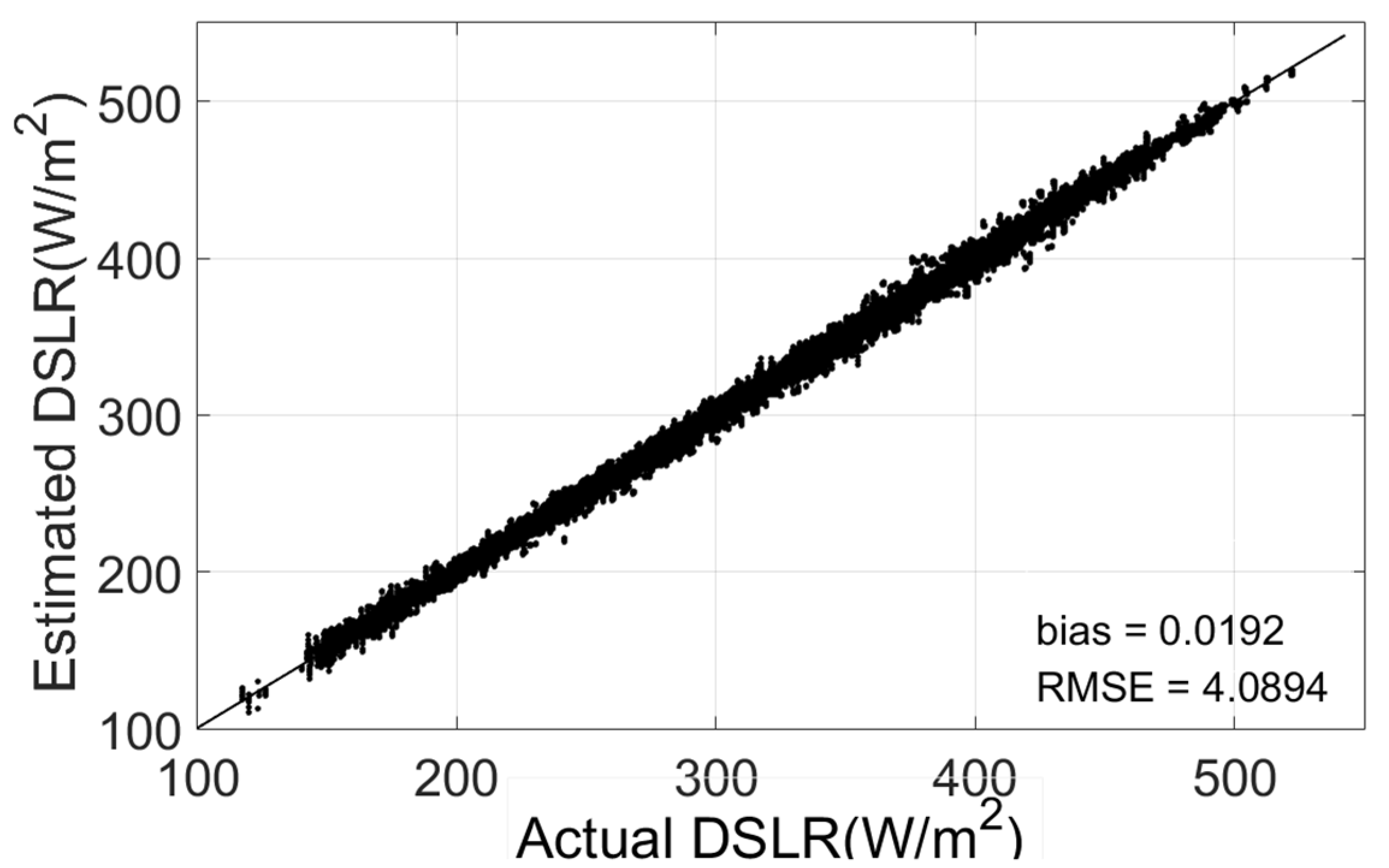
4.1. The Performance of GA-ANN Algorithm

To test the performance of the GA-ANN algorithm under cloudy-sky conditions, the simulated dataset was randomly divided into two groups: one group randomly selected 80% of the simulated dataset as a training dataset to establish the GA-ANN model, and the other group randomly selected 20% as a testing dataset to verify the fitting quality of the algorithm. Figure 2 compares the simulated DSLR (MODTRAN 5 simulated DSLR) and those estimated using the GA-ANN model. The DSLR can be estimated using the GA-ANN model, where bias (estimated minus simulated DSLR) is 0.02 W/m² and where the Root Mean Square Error (RMSE) is 4.09 W/m². The self-verification results show that the DSLR estimation model established by the GA-ANN algorithm can achieve good accuracy under cloudy-sky conditions.

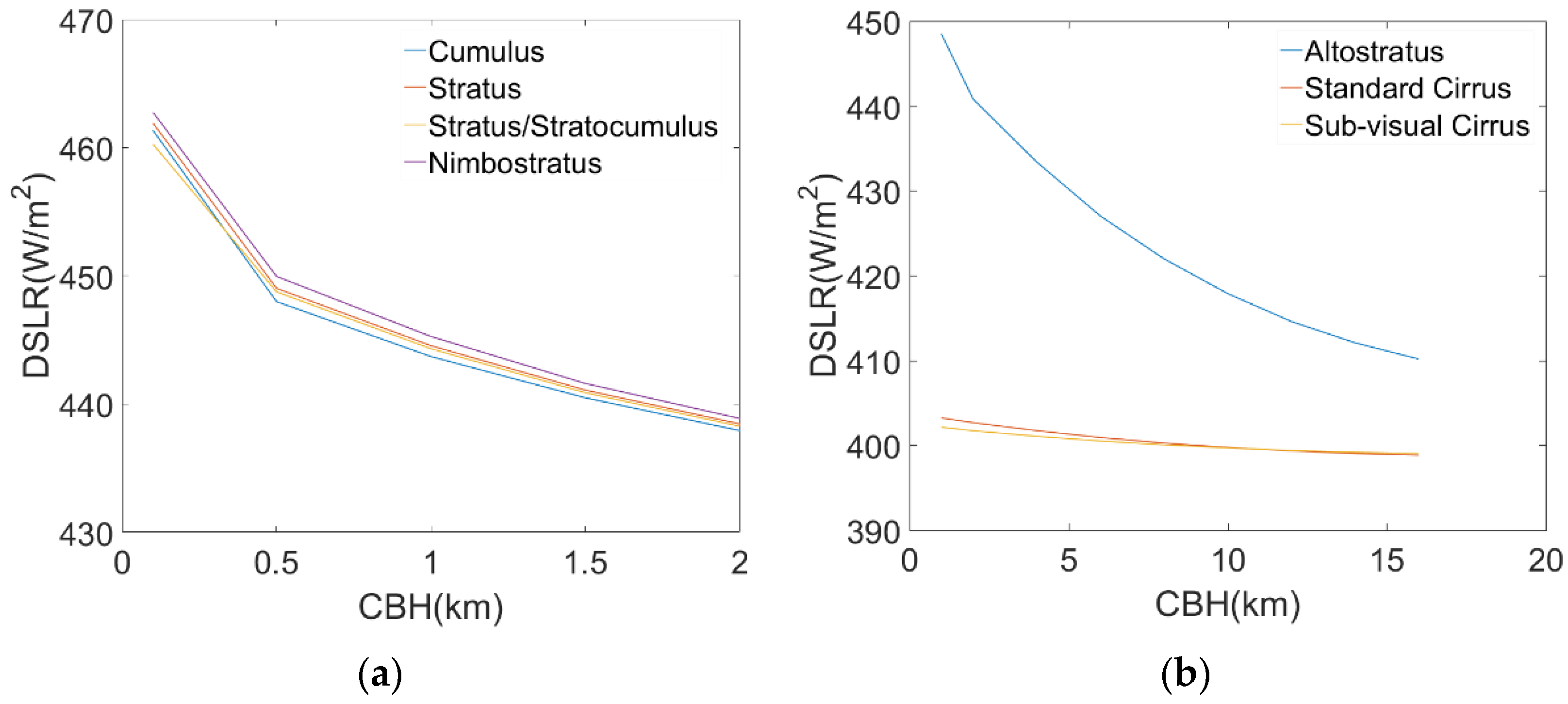
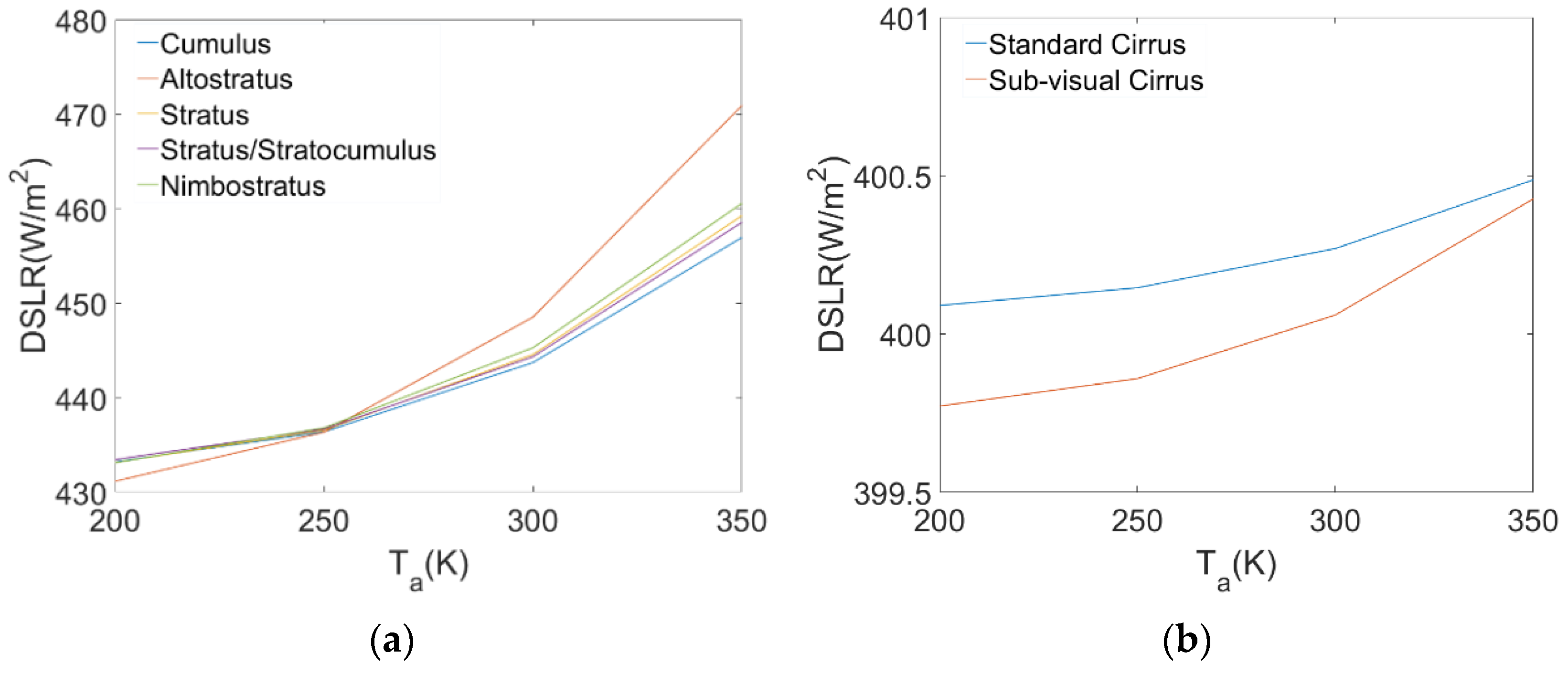
4.2. Sensitivity Analysis

DSLR estimation under cloudy-sky conditions is related to many parameters, such as the atmosphere and clouds. It is necessary to analyze the input data to determine the parameters that are most sensitive to DSLR. Tang and Li [25] analyzed the sensitivity of several thermal infrared bands of MODIS to DSLR, and the results showed that MODIS bands 28, 29, 31, 33, 34, and 36 could be used as input parameters. Wang et al. [29] proposed that the WVC and VZA were crucial for the estimated DSLR; therefore, these parameters were also determined for the input part of the GA-ANN.

CBH is a key parameter for characterizing the cloud radiation effect [33]; therefore, it was used as a required input parameter. In addition to cloud parameters, the greatest uncertainty of DSLR estimation comes from atmospheric parameters such as $T_a$ and WVC [34]. Due to this, $T_a$ was determined by the input parameters. Further, the influence of different $T_a$ and CBH values on the DSLR was quantitatively analyzed. The atmospheric radiative transfer model, MODTRAN 5, was used to set different $T_a$ and CBH values to simulate the effect on DSLR. The controlled variable method was used to uniformly set other MODTRAN variables to fixed values. The cloud model in MODTRAN includes five water cloud and two ice cloud types. The water clouds are cumulus, altostratus, stratus, stratus/stratocumulus, and nimbostratus, and the ice clouds are standard cirrus and subvisual cirrus. Cumulus, stratus, stratus/stratocumulus, and nimbostratus are low clouds. The CBH was set to model a dynamic change from 0.1 to 2 km. Altostratus, standard cirrus, and subvisual cirrus belong to high clouds, and the CBH was set to model a dynamic change from 1 to 16 km. In addition, to analyze the influence of $T_a$ on DSLR, $T_a$ was set in the range of 200 to 350 K.

As shown in

Table 4. DSLR affected by CBH and $T_a$.

	DSLR Affected by CBH			DSLR Affected by $T_a$
	Max (W/m2)	Min (W/m2)	Difference (W/m2)	Max (W/m2)	Min (W/m2)	Difference (W/m2)
Cumulus	461.348	437.934	23.414	456.952	433.198	23.754
Altostratus	448.52	410.177	38.343	470.913	431.144	39.769
Stratus	461.914	438.454	23.460	459.25	433.133	26.117
Stra-tus/Stratocumulus	460.272	438.273	21.999	458.555	433.44	25.115
Nimbostratus	462.762	438.882	23.880	460.568	433.106	27.462
Standard cirrus	403.231	398.846	4.385	400.486	400.089	0.397
Subvisual cirrus	402.139	399.032	3.107	400.426	399.771	0.655

, under the influence of different cloud types, the DSLR changed significantly with changes in CBH and $T_a$. Figure 3 shows the changes in DSLR with CBH under different types of clouds. Combining Figure 3 and Table 4, the data show that the relationships between DSLR and CBH are similar for various cloud types. With an increase in CBH, the DSLR gradually decreased. This is because as CBH increased, the cloud base temperature gradually decreased, resulting in a decrease in the radiation emitted from the cloud base. We also found that altostratus clouds had the largest range of variation, measured at 38.343 W/m². The variation in cirrus clouds was smaller, less than 5 W/m², and the various values of the remaining types of clouds were greater than 20 W/m². Figure 4 shows the trend of DSLR changes with $T_a$. As $T_a$ increased from 200 to 350 K, the DSLR affected by different cloud types also gradually increased. Similarly, we found that the variation range of cirrus clouds was small, and typically less than 1 W/m². For the other types of clouds, the DSLR changes with $T_a$ were greater than 20 W/m². From the above analysis, it can be concluded that the DSLR is sensitive to the CBH and $T_a$. Therefore, CBH and $T_a$ should be used as necessary input parameters when establishing a DSLR estimation algorithm.

5. Validation

5.1. Validation Using in Situ Measurements

Five sites were used to validate the proposed DSLR estimation algorithm. They are the Yingke and Huazhaizi sites of WATER, the Xiyinghe and Linze sites of CARN, and the Huailai site of HAIHE. At each site, six bands of TOA radiance, WVC, and VZA were extracted from MODIS data. $T_a$, CBH, and CF were obtained from the ERA5 reanalysis data. In this study, CF obtained from the reanalysis data was used for two main reasons: first, to ensure the CF is matched to CBH and $T_a$, and second to facilitate the comparison with Bisht and Bras’s [35] model in the later section. Then, according to the GA-ANN model, the DSLR of the clear-sky coverage area and cloud coverage area in cloudy pixels were calculated. Finally, the DSLR under cloudy-sky conditions was obtained using Equation (1). Note that cloudy-sky observations were identified using the MODIS cloud product. Only the cloudy-sky data were retained, and during the validation process, the ground-measured DSLRs that were closest to the MODIS satellite overpass time were adopted.

Figure 5 shows a scatterplot of the estimated cloudy-sky DSLR vs. the measured values at the five sites. It is evident that the proposed model can produce a reasonable DSLR under cloudy-sky conditions at all sites with a bias of <10 W/m² and an RMSE of <35 W/m². Overall, similar accuracy was observed at each site, with biases and RMSE’s ranging from −1.28 to 13.57 W/m² and 31.33 to 39.20 W/m², respectively. There is a large RMSE (39.20 W/m²) at the Huailai site and a large bias (−13.57 W/m²) at the Xiyinghe site. The Xiyinghe site was located in a rugged area with a large surface elevation, which led to a large bias. According to the histogram of the error distribution (Figure 6), the new method has different degrees of underestimation at different sites. This is due to the negative bias at high altitudes when estimating DSLRs based on the TOA radiance. The Yingke, Huazhaizi, Linze, and Xiyinghe sites in this study are all located in high-altitude areas, resulting in the underestimation of the estimation results. Some researchers [36] found that when the temperature difference between the surface and the atmosphere is large, the DSLR estimated by the parametric model is prone to overestimation. The sites in the Heihe River Basin (Yinghe site, Huazhizi site) and the Qilian Mountains Basin (Linze site, Xiyinghe site) are located in arid areas, with low vegetation coverage and a large temperature difference between the surface and the atmosphere, which is the reason for the overestimation of the estimated value. The high value of the estimation occurs in summer, when the temperature difference between the surface and the atmosphere is larger, which leads to overestimation in the high-value regions.

5.2. Comparison with Existing Methods

As mentioned above, a variety of algorithms exist for estimating the DSLR under cloudy-sky conditions. Bisht and Bras’s [35] method was selected for comparison in this study. Bisht and Bras’s [35] method is expressed as follows:

$$DSL{R}_{cloudy}=\sigma {\epsilon }_a{T}_a^4+\sigma \left(1-{\epsilon }_a\right){\epsilon }_c{T}_c^4$$

(4)

where σ is the Stefan–Boltzmann constant ($5.67\times 10{}^{-8}\mathrm{W}·{\mathrm{m}}^{-2}·{\mathrm{K}}^{-4}$), ${\epsilon }_a$ is the air emissivity at near-surface, $T_a$ is the near-surface air temperature, ${\epsilon }_c$ is the cloud emissivity, and $T_c$ is the cloud base temperature. Note that ${\epsilon }_c$ was set to 1, and ${\epsilon }_a$ was calculated using the bulk scheme of Prata [37]:

$${\epsilon }_a=1-\left(1+\xi \right)\exp \left(-\sqrt{\left(1.2+3\xi \right)}\right)$$

(5)

$$\xi =\frac{46.5}{T_a}{e}_0$$

(6)

where $e_0$ is the near-surface vapor pressure (hPa), which can be computed using the dew point temperature according to the Clausius–Clapeyron equation:

$$e_0=6.11\exp \left[\frac{L_V}{R_V}\left(\frac{1}{T_0}-\frac{1}{T_d}\right)\right]$$

(7)

where $L_V=2.5\times {10}^6{\mathrm{J}\mathrm{kg}}^{-1}$ is the latent heat of vaporization, $R_V=461\mathrm{J}·{\mathrm{kg}}^{-1}{\mathrm{K}}^{-1}$ is the gas constant for water vapor, $T_0=273.15\mathrm{K}$, and $T_d$ is the dew point temperature (K). Based on the same data as in Section 4.1, Bisht and Bras‘s [35] method was tested using ERA5 reanalysis data. A scatter diagram comparing the estimated results and site measurements is shown in Figure 7. The performance of Bisht and Bras’s [35] method at each site is summarized in

Table 5. The performance of Bisht and Bras’s [35] method.

Sites	Bias (W/m2)	RMSE (W/m2)	No. of Points
Huailai	20.27	36.04	121
Yingke	36.82	45.62	98
Huaizhazi	30.82	40.30	112
Linze	42.64	47.33	135
Xiyinghe	24.08	38.23	187

.

It can be seen from Figure 7 that Bisht and Bras’s [35] method exhibits a relatively large bias (30.28 W/m²) and RMSE (41.39 W/m²). Overall, the comparison of Bisht and Bras’s [35] method with site measurement data showed a large overestimation, which is consistent with the results of Wang et al. [11]. From Table 5, it is apparent that Bisht and Bras’s [35] method overestimates at each site, and its RMSE is larger than that of the newly proposed method.

In addition, we compared the results with existing estimates of other methods under cloudy-sky conditions. Currently, the main DSLR estimation methods under cloudy-sky conditions can be divided into empirical algorithms based on cloud fraction and single-layer cloud models. Yu et al. [38] validated two common estimation methods. Wang et al. [11] and Yang and Cheng [12] used the single-layer cloud model to estimate DSLR by calculating the CBH and combining it with temperature profile data. The results were compared according to these two classifications (

Table 6. Comparisons of DSLR estimates in this study with existing studies.

Algorithms	Model	Bias (W/m2)	RMSE (W/m2)
This study	GA-ANN	−9.18	34.88
Yu et al. [38]	Empirical Algorithms Based on Cloud Fraction (Crawford and Duchon [3])	35.8	52.6
	Empirical Algorithms Based on Cloud Fraction (Iziomon et al. [39])	6.4	40.4
	Empirical Algorithms Based on Cloud Fraction (Josey et al. [40])	−34.4	48.4
	Empirical Algorithms Based on Cloud Fraction (Trigo et al. [41])	3.3	32.3
	Single-Layer Cloud Model (Schmetz et al. [42])	21.7	42.5
	Single-Layer Cloud Model (Gupta et al. [43])	15.9	33.3
	Single-Layer Cloud Model (Diak et al. [44])	24.3	41.8
Wang et al. [11]	Single-Layer Cloud Model	−7.7	32.8
Yang and Cheng [12]	Single-Layer Cloud Model	5.42	30.3

). The DSLR estimated by these algorithms greatly varied. In contrast to the above studies, this study used simulated data to establish the GA-ANN algorithm and then combined remote sensing data and ERA5 reanalysis data to estimate the DSLR under cloudy-sky conditions. Comparing these methods, this study obtained a similar accuracy, with a bias of −9.18 W/m² and a RMSE of 34.88 W/m².

6. Discussion

DSLR under cloudy-sky conditions is composed of two parts: one is from the contribution of the sub-cloud atmosphere and the other is from the radiation contributed by clouds. The contribution of the sub-cloud atmosphere is impacted by atmospheric emissivity, which controls the penetration of the DSLR contributed by the atmosphere and the DSLR emitted by the cloud. Some studies [3,39,45] have proposed the use of the function of $T_a$ and water vapor pressure to express atmospheric emissivity. Some studies [46,47] have only used $T_a$ to calculate atmospheric emissivity. In either case, there are two crucial variables: one being the water vapor pressure and the other being $T_a$. In this study, WVC was used to reflect changes in water vapor. WVC and $T_a$ were added to the GA-ANN model as input parameters. The WVC was obtained from MOD05 products, and the $T_a$ was from ERA5 reanalysis data. Wang et al. [29] analyzed the influence of WVC on DSLR estimation under aerosol conditions, and the results showed that WVC was crucial for quantifying aerosol longwave radiative forcing. According to Section 4.2, DSLR also has a strong positive correlation with $T_a$, since the spatial resolution of $T_a$ in ERA5 reanalysis data was 0.25°, which is relatively imprecise, leading to great uncertainty in the estimation results. In addition, this study used the nearest neighbor method to match different data, which is bound to cause certain errors.

The CBH is a key parameter for measuring the radiation effect of cloud contributions in DSLR estimation. One of the challenges in surface radiation estimation is the proper determination of the CBH. An error of 100 m in the CBH can generate a DSLR error of 1.5 W/m² [48,49]. In general, the influence of multi-layer clouds is not considered in high-resolution DSLR estimation because clouds at different heights are generally completely overlapped on the kilometer scale. The DSLR is mainly affected by the lowest-layer cloud; however, when the lowest-layer cloud is not a black body, the DSLR estimation under cloudy-sky conditions is affected by upper-layer clouds. Regrettably, it is difficult to identify and detect multi-layer clouds, which leads to uncertainties in the estimation of CBH.

To further analyze the correlation between CBH, $T_a$, and DSLR, we plotted the CBH and estimated DSLR, and plotted $T_a$ and estimated DSLR. The results are shown in Figure 8. Although CBH affects the thermal radiation emission capacity of clouds, its linear correlation with the estimated DSLR is weak. In contrast, the estimated DSLR has a strong linear relationship with $T_a$, indicating that $T_a$ is still an important factor affecting the DSLR even under cloudy-sky conditions.

7. Conclusions

In this study, a new method for estimating DSLR under cloudy-sky conditions was established by combining the neural network model with the radiance of TOA, VZA, and WVC from MODIS satellite data along with the $T_a$ and CBH from ERA5 reanalysis data. Based on radiative transfer theory, the GA-ANN algorithm was developed using data simulated by MODTRAN 5. Self-verified results showed that the instantaneous DSLR bias and RMSE estimated by this new method were 0.02 and 4.09 W/m², respectively. To verify the accuracy and reliability of the new method, five field observation sites in three observation networks were used to validate the DSLR estimation. The results showed that the new method can achieve good accuracy, with a bias of −9.18 W/m² and a RMSE of 34.88 W/m².

To further verify the proposed method, the algorithm proposed by Bisht and Bras [35] was combined with ERA5 reanalysis data to estimate the DSLR under cloudy-sky conditions. Comparisons of the results showed that the new method is superior to this method at all sites. In addition, this study compared various DSLR estimation methods summarized and validated by Yu et al. [38] and the single-layer cloud estimation models used by Wang et al. [11] and Yang and Cheng [12]. The proposed new method can achieve accuracy similar to that of the above methods.

References

1. Deardoff, J.W. Efficient prediction of ground surface temperature and moisture, with inclusion of a layer of vegetation. J. Geophys. Res. Atmos. 1987, 96, 541–550. [Google Scholar]
2. Aladosarboledas, I.; Vida, J.; Olmo, F.J. The estimation of thermal atmospheric radiation under cloudy conditions. Int. J. Climatol. 1995, 15, 589. [Google Scholar]
3. Crawford, T.M.; Duchon, C.E. An improved parameterization for estimating effective atmospheric emissivity for use in calculating daytime downwelling longwave radiation. J. Appl. Meteorol. 1999, 38, 474–480. [Google Scholar] [CrossRef]
4. Lhomme, J.P.; Vacher, J.J.; Rocheteau, A. Estimating downward long-wave radiation on the Andean Altiplano. Agric. For. Meteorol. 2007, 145, 139–148. [Google Scholar] [CrossRef]
5. Rooney, G.G. Modelling of downwelling long-wave radiation using cloud fraction obtained from laser cloud-base measurements. Atmos. Sci. Lett. 2005, 6, 160–163. [Google Scholar] [CrossRef]
6. Zhong, L.; Zou, M.; Ma, Y.; Huang, Z.; Xu, K.; Wang, X.; Ge, N.; Cheng, M. Estimation of Downwelling Shortwave and Longwave Radiation in the Tibetan Plateau Under All-Sky Conditions. J. Geophys. Res. Atmos. 2019, 124, 11086–11102. [Google Scholar] [CrossRef]
7. Cheng, J.; Yang, F.; Guo, Y. A Comparative Study of Bulk Parameterization Schemes for Estimating Cloudy-Sky Surface Downward Longwave Radiation. Remote Sens. 2019, 11, 528. [Google Scholar] [CrossRef] [Green Version]
8. Liu, M.; Zheng, X.; Zhang, J.; Xia, X. A revisiting of the parametrization of downward longwave radiation in summer over the Tibetan Plateau based on high-temporal-resolution measurements. Atmos. Chem. Phys. 2020, 20, 4415–4426. [Google Scholar] [CrossRef] [Green Version]
9. Dilley, A.C.; O’Brien, D.M. Estimating downward clear sky long-wave irradiance at the surface from screen temperature and precipitable water. Q. J. R. Meteorol. Soc. 1998, 124, 1391–1401. [Google Scholar] [CrossRef]
10. Jacobs, J.D. Radiation Climate of Broughton Island. In Energy Budget Studies in Relation to Fast-Ice Breakup Processes in Davis Strait; Barry, R.G., Jacobs, J.D., Eds.; Occasional Paper No. 26; Institute of Arctic and Alp Research, University of Colorado: Boulder, CO, USA, 1978; pp. 105–120. [Google Scholar]
11. Wang, T.; Shi, J.; Yu, Y.; Husi, L.; Gao, B.; Zhou, W.; Ji, D.; Zhao, T.; Xiong, C.; Chen, L. Cloudy-sky land surface longwave downward radiation (LWDR) estimation by integrating MODIS and AIRS/AMSU measurements. Remote Sens. Environ. 2018, 205, 100–111. [Google Scholar] [CrossRef]
12. Yang, F.; Cheng, J. A framework for estimating cloudy sky surface downward longwave radiation from the derived active and passive cloud property parameters. Remote Sens. Environ. 2020, 248, 111972. [Google Scholar] [CrossRef]
13. Ahn, S.-H.; Lee, K.-T.; Rim, S.-H.; Zo, I.-S.; Kim, B.-Y. Surface Downward Longwave Radiation Retrieval Algorithm for GEO-KOMPSAT-2A/AMI. Asia-Pac. J. Atmos. Sci. 2018, 54, 237–251. [Google Scholar] [CrossRef]
14. Gupta, S.K.; Darnell, W.L.; Wilber, A.C. A Parameterization for Longwave Surface Radiation from Satellite Data—Recent Improvements. J. Appl. Meteorol. 1992, 31, 1361–1367. [Google Scholar] [CrossRef] [Green Version]
15. Wang, T.; Shi, J.; Ma, Y.; Letu, H.; Li, X. All-sky longwave downward radiation from satellite measurements: General parameterizations based on LST, column water vapor and cloud top temperature. ISPRS J. Photogramm. Remote Sens. 2020, 161, 52–60. [Google Scholar] [CrossRef]
16. Savtchenko, A.; Ouzounov, D.; Ahmad, S.; Acker, J.; Leptoukh, G.; Koziana, J.; Nickless, D. Terra and aqua MODIS products available from NASA GES DAAC. Adv. Space Res. 2004, 34, 710–714. [Google Scholar] [CrossRef]
17. Wolfe, R.E.; Nishihama, M.; Fleig, A.J.; Kuyper, J.A.; Roy, D.P.; Storey, J.C.; Patt, F.S. Achieving sub-pixel geolocation accuracy in support of MODIS land science. Remote Sens. Environ. 2002, 83, 31–49. [Google Scholar] [CrossRef]
18. Xu, T.R.; Liu, S.M.; Xu, L.; Chen, Y.J.; Jia, Z.Z.; Xu, Z.W.; Nielson, J. Temporal Upscaling and Reconstruction of Thermal Remotely Sensed Instantaneous Evapotranspiration. Remote Sens. 2015, 7, 3400–3425. [Google Scholar] [CrossRef] [Green Version]
19. Li, X.; Li, X.; Li, Z.; Ma, M.; Wang, J.; Xiao, Q.; Liu, Q.; Che, T.; Chen, E.; Yan, G. Watershed Allied Telemetry Experimental Research. J. Geophys. Res. Atmos. 2012, 114, 2191–2196. [Google Scholar] [CrossRef] [Green Version]
20. Liu, S.M.; Li, X.; Xu, Z.W.; Che, T.; Xiao, Q.; Ma, M.G.; Liu, Q.H.; Jin, R.; Guo, J.W.; Wang, L.X.; et al. The Heihe Integrated Observatory Network: A Basin-Scale Land Surface Processes Observatory in China. Vadose Zone J. 2018, 17, 1–21. [Google Scholar] [CrossRef]
21. Liu, S.M.; Xu, Z.W.; Wang, W.Z.; Jia, Z.Z.; Zhu, M.J.; Bai, J.; Wang, J.M. A comparison of eddy-covariance and large aperture scintillometer measurements with respect to the energy balance closure problem. Hydrol. Earth Syst. Sci. 2011, 15, 1291–1306. [Google Scholar] [CrossRef] [Green Version]
22. Liu, S.M.; Xu, Z.W.; Zhu, Z.L.; Jia, Z.Z.; Zhu, M.J. Measurements of evapotranspiration from eddy-covariance systems and large aperture scintillometers in the Hai River Basin, China. J. Hydrol. 2013, 487, 24–38. [Google Scholar] [CrossRef]
23. Guo, A.L.; Liu, S.M.; Zhu, Z.L.; Xu, Z.W.; Xiao, Q.; Ju, Q.; Zhang, Y.; Yang, X.F. Impact of Lake/Reservoir Expansion and Shrinkage on Energy and Water Vapor Fluxes in the Surrounding Area. J. Geophys. Res. Atmos. 2020, 125, e2020JD032833. [Google Scholar] [CrossRef]
24. Berk, A.; Bernstein, L.S.; Anderson, G.P.; Acharya, P.K.; Robertson, D.C.; Chetwynd, J.H.; Adler-Golden, S.M. MODTRAN cloud and multiple scattering upgrades with application to AVIRIS. Remote Sens. Environ. 1998, 65, 367–375. [Google Scholar] [CrossRef]
25. Tang, B.; Li, Z.-L. Estimation of instantaneous net surface longwave radiation from MODIS cloud-free data. Remote Sens. Environ. 2008, 112, 3482–3492. [Google Scholar] [CrossRef]
26. Wang, W.; Liang, S. Estimation of high-spatial resolution clear-sky longwave downward and net radiation over land surfaces from MODIS data. Remote Sens. Environ. 2009, 113, 745–754. [Google Scholar] [CrossRef]
27. Yan, G.J.; Wang, T.X.; Jiao, Z.H.; Mu, X.H.; Zhao, J.; Chen, L. Topographic radiation modeling and spatial scaling of clear-sky land surface longwave radiation over rugged terrain. Remote Sens. Environ. 2016, 172, 15–27. [Google Scholar] [CrossRef]
28. Wang, J.; Tang, B.-H.; Zhang, X.-Y.; Wu, H.; Li, Z.-L. Estimation of Surface Longwave Radiation over the Tibetan Plateau Region Using MODIS Data for Cloud-Free Skies. IEEE J. Sel. Top. Appl. Earth Obs. Remote Sens. 2014, 7, 3695–3703. [Google Scholar] [CrossRef]
29. Wang, C.; Tang, B.-H.; Wu, H.; Tang, R.; Li, Z.-L. Estimation of Downwelling Surface Longwave Radiation under Heavy Dust Aerosol Sky. Remote Sens. 2017, 9, 207. [Google Scholar] [CrossRef] [Green Version]
30. Suzuki, K. Artificial Neural Networks—Methodological Advances and Biomedical Applications; IntechOpen: London, UK, 2011. [Google Scholar]
31. Peng, Z.; Letu, H.S.; Wang, T.X.; Shi, C.; Zhao, C.F.; Tana, G.G.; Zhao, N.Z.; Dai, T.; Tang, R.L.; Shang, H.Z.; et al. Estimation of shortwave solar radiation using the artificial neural network from Himawari-8 satellite imagery over China. J. Quant. Spectrosc. Radiat. Transf. 2020, 240, 106672. [Google Scholar] [CrossRef]
32. Si, M.L.; Tang, B.H.; Li, Z.L.; Nerry, F.; Zhang, X.; Shang, G.F. An Artificial Neuron Network With Parameterization Scheme for Estimating Net Surface Shortwave Radiation From Satellite Data Under Clear Sky—Application to Simulated GF-5 Data Set. IEEE Trans. Geosci. Remote Sens. 2021, 59, 4262–4272. [Google Scholar] [CrossRef]
33. Stephens, G.L.; Wild, M.; Stackhouse, P.W.; L’Ecuyer, T.; Kato, S.; Henderson, D.S. The Global Character of the Flux of Downward Longwave Radiation. J. Clim. 2012, 25, 2329–2340. [Google Scholar] [CrossRef] [Green Version]
34. Wang, K.C.; Dickinson, R.E. Global atmospheric downward longwave radiation at the surface from ground-based observations, satellite retrievals, and reanalyses. Rev. Geophys. 2013, 51, 150–185. [Google Scholar] [CrossRef]
35. Bisht, G.; Bras, R.L. Estimation of net radiation from the MODIS data under all sky conditions: Southern Great Plains case study. Remote Sens. Environ. 2010, 114, 1522–1534. [Google Scholar] [CrossRef]
36. Yu, S.; Xin, X.; Liu, Q. Estimation of clear-sky longwave downward radiation from HJ-1B thermal data. Sci. China Earth Sci. 2012, 56, 829–842. [Google Scholar] [CrossRef]
37. Prata, A.J. A new long-wave formula for estimating downward clear-sky radiation at the surface. Q. J. R. Meteorol. Soc. 1996, 122, 1127–1151. [Google Scholar] [CrossRef]
38. Yu, S.; Xin, X.; Liu, Q.; Zhang, H.; Li, L. Comparison of Cloudy-Sky Downward Longwave Radiation Algorithms Using Synthetic Data, Ground-Based Data, and Satellite Data. J. Geophys. Res. Atmos. 2018, 123, 5397–5415. [Google Scholar] [CrossRef]
39. Iziomon, M.G.; Mayer, H.; Matzarakis, A. Downward atmospheric longwave irradiance under clear and cloudy skies: Measurement and parameterization. J. Atmos. Sol.-Terr. Phys. 2003, 65, 1107–1116. [Google Scholar] [CrossRef]
40. Josey, S.A.; Pascal, R.W.; Taylor, P.K.; Yelland, M.J. A new formula for determining the atmospheric longwave flux at the ocean surface at mid-high latitudes. J. Geophys. Res. Ocean. 2003, 108, C4. [Google Scholar] [CrossRef]
41. Trigo, I.F.; Barroso, C.; Viterbo, P.; Freitas, S.C.; Monteiro, I.T. Estimation of downward long-wave radiation at the surface combining remotely sensed data and NWP data. J. Geophys. Res. Atmos. 2010, 115, D24. [Google Scholar] [CrossRef]
42. Schmetz, P.; Schmetz, J.; Raschke, E. Estimation of Daytime Downward Longwave Radiation at The Surface From Satellite And Grid Point Data. Theor. Appl. Climatol. 1986, 37, 136–149. [Google Scholar] [CrossRef]
43. Gupta, S.K.; Kratz, D.P.; Stackhouse, P.W.; Wilber, A.C.; Zhang, T.P.; Sothcott, V.E. Improvement of Surface Longwave Flux Algorithms Used in CERES Processing. J. Appl. Meteorol. Climatol. 2010, 49, 1579–1589. [Google Scholar] [CrossRef]
44. Diak, G.R.; Bland, W.L.; Mecikalski, J.R.; Anderson, M.C. Satellite-based estimates of longwave radiation for agricultural applications. Agric. For. Meteorol. 2000, 103, 349–355. [Google Scholar] [CrossRef]
45. Gao, B.-C.; Kaufman, Y.J. Water vapor retrievals using Moderate Resolution Imaging Spectroradiometer (MODIS) near-infrared channels. J. Geophys. Res. Atmos. 2003, 108, 4389. [Google Scholar] [CrossRef]
46. Swinbank, W.C. Long-wave Radiation From Clear Skies. Q. J. R. Meteorol. Soc. 1963, 89, 339–348. [Google Scholar] [CrossRef]
47. Idso, S.B.; Jackson, R.D. Thermal Radiation From Atmosphere. J. Geophys. Res. 1969, 74, 5397–5403. [Google Scholar] [CrossRef]
48. Trenberth, K.E.; Fasullo, J.T.; Kiehl, J. Earth’s Global Energy Budget. Bull. Am. Meteorol. Soc. 2009, 90, 311–323. [Google Scholar] [CrossRef]
49. Viudez-Mora, A.; Costa-Suros, M.; Calbo, J.; Gonzalez, J.A. Modeling atmospheric longwave radiation at the surface during overcast skies: The role of cloud base height. J. Geophys. Res. Atmos. 2015, 120, 199–214. [Google Scholar] [CrossRef] [Green Version]
Figure 1. Spatial distribution of the observation sites. (a) Location of the all sites; (b) Location of the Huailai site; (c) Location of the four sites (Linze, Yingke, Huazhaizi, and Xiyinghe).
Remotesensing 14 02716 g001
Figure 2. The comparison of simulated DSLR (MODTRAN 5 simulated DSLR) and those estimated using the GA-ANN model.
Remotesensing 14 02716 g002
Figure 3. Changes of DSLR with different CBH. (a) DSLR vs. CBH for low clouds, (b) DSLR vs. CBH for high clouds.
Remotesensing 14 02716 g003
Figure 4. Changes of DSLR with different T a . (a) DSLR vs. Ta for five types of clouds (Cumulus, Altostratus, Stratus, Stratus/Stratocumulus, and Nimbostratus), (b) DSLR vs. Ta for Standard Cirrus and Sub-visual Cirrus.
Remotesensing 14 02716 g004
Figure 5. Scatterplot of the derived cloudy-sky DSLR vs. ground DSLR measurements.
Remotesensing 14 02716 g005
Figure 6. The error histogram of the proposed method at all sites.
Remotesensing 14 02716 g006
Figure 7. Scatterplot of the derived cloudy-sky DSLR vs. ground DSLR measurements from Bisht and Bras’s [35] method at all sites.
Remotesensing 14 02716 g007
Figure 8. Scatterplot of the estimated DSLR vs. cloud base height and near-surface air temperature.
Remotesensing 14 02716 g008