Article

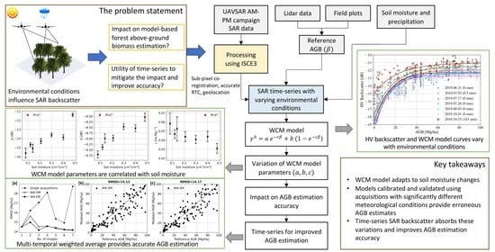
Assessment of Forest Biomass Estimation from Dry and Wet SAR Acquisitions Collected during the 2019 UAVSAR AM-PM Campaign in Southeastern United States

Jet Propulsion Laboratory, California Institute of Technology, Pasadena, CA 91109, USA
*
Author to whom correspondence should be addressed.
Remote Sens. 2020, 12(20), 3397; https://doi.org/10.3390/rs12203397
Submission received: 26 August 2020 / Revised: 10 October 2020 / Accepted: 12 October 2020 / Published: 16 October 2020
(This article belongs to the Special Issue Forest Biomass and Carbon Observation with Remote Sensing)

Abstract

:
Forest above-ground biomass (AGB) estimation from SAR backscatter is affected by varying imaging and environmental conditions. This paper quantifies and compares the performance of forest biomass estimation from L-band SAR backscatter measured selectively under dry and wet conditions during the 2019 AM-PM NASA airborne campaign. Seven Uninhabited Aerial Vehicle Synthetic Aperture Radar (UAVSAR) images acquired between June and October 2019 over a temperate deciduous forest in Southeastern United States with varying moisture and precipitation conditions are examined in conjunction with LIDAR and field measurements. Biomass is estimated by fitting a 3-parameter modified Water Cloud Model (WCM) to radiometric terrain corrected SAR backscatter. Our experiment is designed to quantify the biomass estimation errors when biomass models are calibrated and validated on varying acquisition conditions (dry or wet). Multi-temporal estimation strategies are also evaluated and compared with single-acquisition estimation approaches. As an outcome, the experiment shows that the WCM model calibrated and validated on single acquisitions adapts to different soil moisture conditions with RMSD up to 18.7 Mg/ha. The AGB estimation performance, however, decreases with RMSD upwards of 30 Mg/ha when the model is cross-validated on moisture and precipitation conditions different than the calibration conditions. Results confirm that calibrating the model over the multi-temporal data using averaged backscatter or weighted combinations of individual AGB estimates, improves the biomass estimation accuracy up to about 20% at L-band. This study helps design biomass cal/val procedures and biomass estimation algorithms for dense time-series to be collected by low-frequency radar missions such as NASA-ISRO SAR (NISAR) and BIOMASS.

Graphical Abstract

1. Introduction

Synthetic aperture radar (SAR) backscatter has been extensively explored for above-ground biomass (AGB) estimation across various forest ecosystems ranging from tropical to boreal [1,2,3,4,5,6,7,8,9]. The sensitivity of SAR backscatter to AGB has been modeled in many studies to estimate forest AGB using empirical [10,11,12], semi-empirical [13] and numerical [14,15] models, and machine learning algorithms [16,17,18]. SAR backscatter is sensitive to AGB up to a saturation level [19], although, for dense forests, a decrease in backscatter above saturation level may be observed [20]. The saturation at a specific biomass is determined by radar frequency along with other factors including polarization and forest conditions [2,4]. L-band SAR backscatter has been extensively used for forest AGB retrieval due to its higher sensitivity to forest AGB (resulting from higher saturation level) [1,2,3,21,22] and availability through various airborne and satellite missions (Seasat, the Shuttle Imaging Radar (SIR-C), Japanese Earth Resources Satellite (JERS), Uninhabited Aerial Vehicle Synthetic Aperture Radar (UAVSAR), Advanced Land Observation Satellite (ALOS) Phased Array type L-band Synthetic Aperture Radar (PALSAR) and its successor ALOS-2/PALSAR-2).
The relationship between SAR backscatter and AGB depends on the dynamic conditions of forest canopies and underlying soil. SAR backscatter is sensitive to changes in forest characteristics [2,13,23,24] and environmental conditions including soil moisture or weather [13,21,25,26,27,28], further impacting the AGB estimation accuracy. Most studies use AGB data estimated from field plots, which might have inherent uncertainties due to allometry [29], geolocation, and inadequate representation of the spatial variability of the forest [30]. Various studies analyze and model the sources of uncertainties in AGB estimation from SAR data [19,30].
Furthermore, L-band backscatter from forests depends on the imaging conditions, in particular, wet or dry state of canopy and soil [2]. Pullianen et al. [31] showed that JERS L-band SAR backscatter over mature boreal forests varied by 1 dB between wet and dry conditions. Harrell et al. [25] reported the sensitivity of SIR-C L-band backscatter-biomass relation in a pine forest to soil moisture variations. Bouvet et al. [4] trained L-band ALOS/PALSAR backscatter on African woodlands in wet and dry seasons to estimate AGB and showed that non-homogeneous environmental conditions (soil moisture changes and precipitation) can lead up to 300% errors in AGB estimates. The wet/dry imaging conditions affect the overall backscatter from forest canopy and ground, and the sensitivity to forest AGB [2,23,25,31]. The integration of multi-temporal SAR acquisitions can reduce the impact of these variations and increase AGB retrieval accuracy [2,3,13,23,24]. To capture the contribution of environmental conditions to backscatter and forest AGB estimation require extensive in situ data and multi-temporal SAR data acquired in varying environmental conditions. However, repeat-pass L-band SAR acquisitions are scarce or have long temporal gaps between acquisitions leading to relatively limited exploration of multi-temporal SAR backscatter data for forest AGB retrieval [1].
This study aims to address this research gap and analyze the effect of varying environmental conditions on SAR backscatter-modeled AGB estimation accuracy. The objectives of this study are to assess (1) the performance of forest AGB estimation from L-band SAR cross-polarized backscatter to changes in acquisition conditions, and (2) the ability of multi-temporal acquisitions to mitigate the impact on AGB estimation. The purpose is to quantify the errors associated with mixing dry and wet acquisitions in the calibration and validation of forest biomass models and assess available mitigation strategies that combine data in multi-temporal SAR stacks. Our investigation uses data collected during the 2019 AM-PM UAVSAR airborne campaign in support of the NASA-ISRO SAR (NISAR) calibration and validation activities [32].
The NISAR mission, scheduled to launch in 2022, will provide unprecedented dense time-series of dual-polarized (HH and HV) L-band SAR data globally, with a repeat-pass of 12 days and a single-look-complex (SLC) spatial resolution finer than 10 m. NISAR will deliver 30 to 60 ascending and descending polarimetric and interferometric acquisitions per year. Based on its science requirements, NISAR L-band backscatter time-series will enable the generation of global AGB maps with a root mean squared error (RMSE) of 20 Mg/ha for at least 80% of forests on Earth with AGB less than 100 Mg/ha.
The organization of the paper is as follows. Section 2 describes the study site and the data-sets used. The Water Cloud Model (WCM) model training and validation are discussed in Section 3. Section 4 presents the data analysis and discusses the effect of soil moisture and precipitation on backscatter and AGB estimation accuracy. The conclusions of the study drawn in Section 5.

2. Data and Study Site

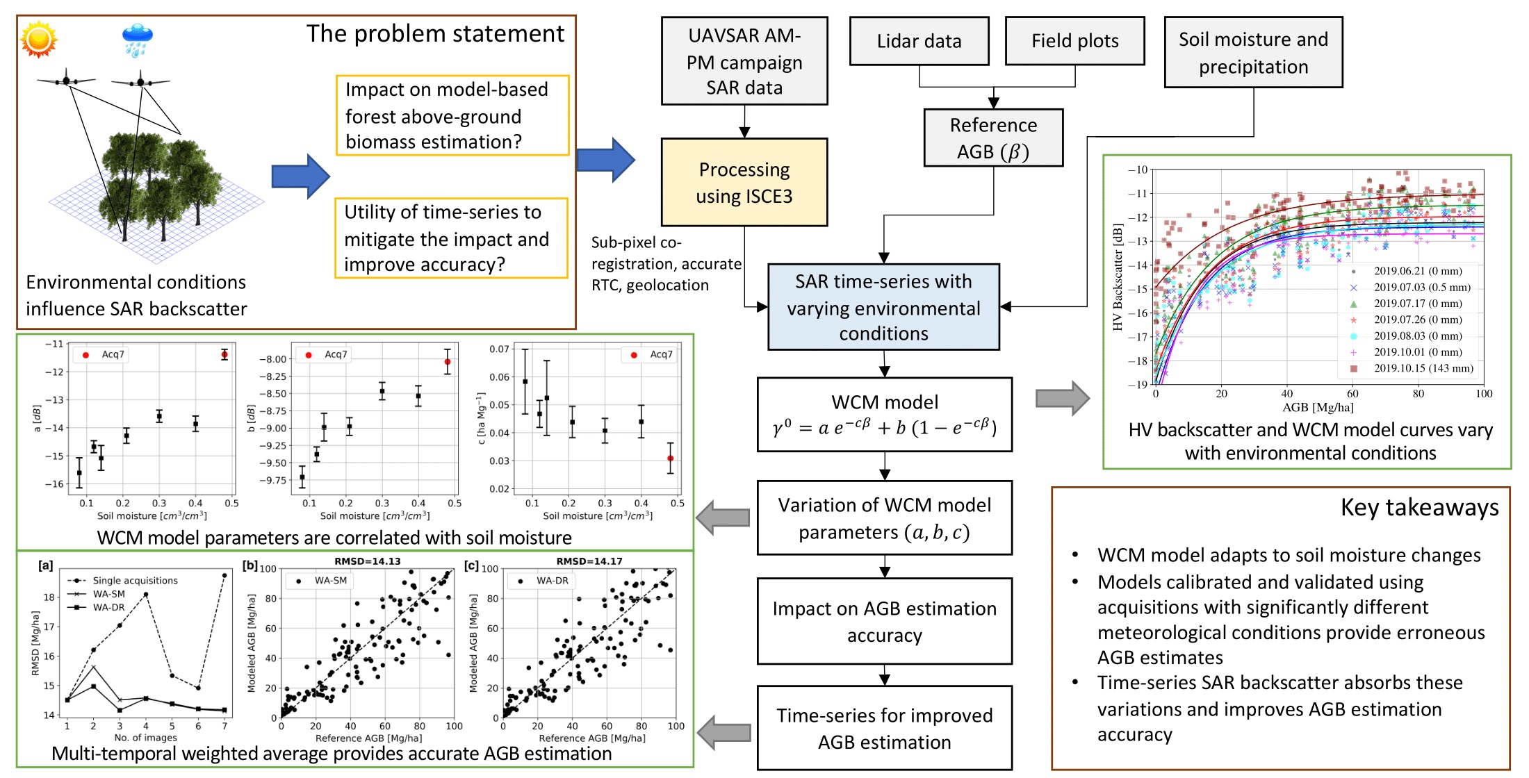
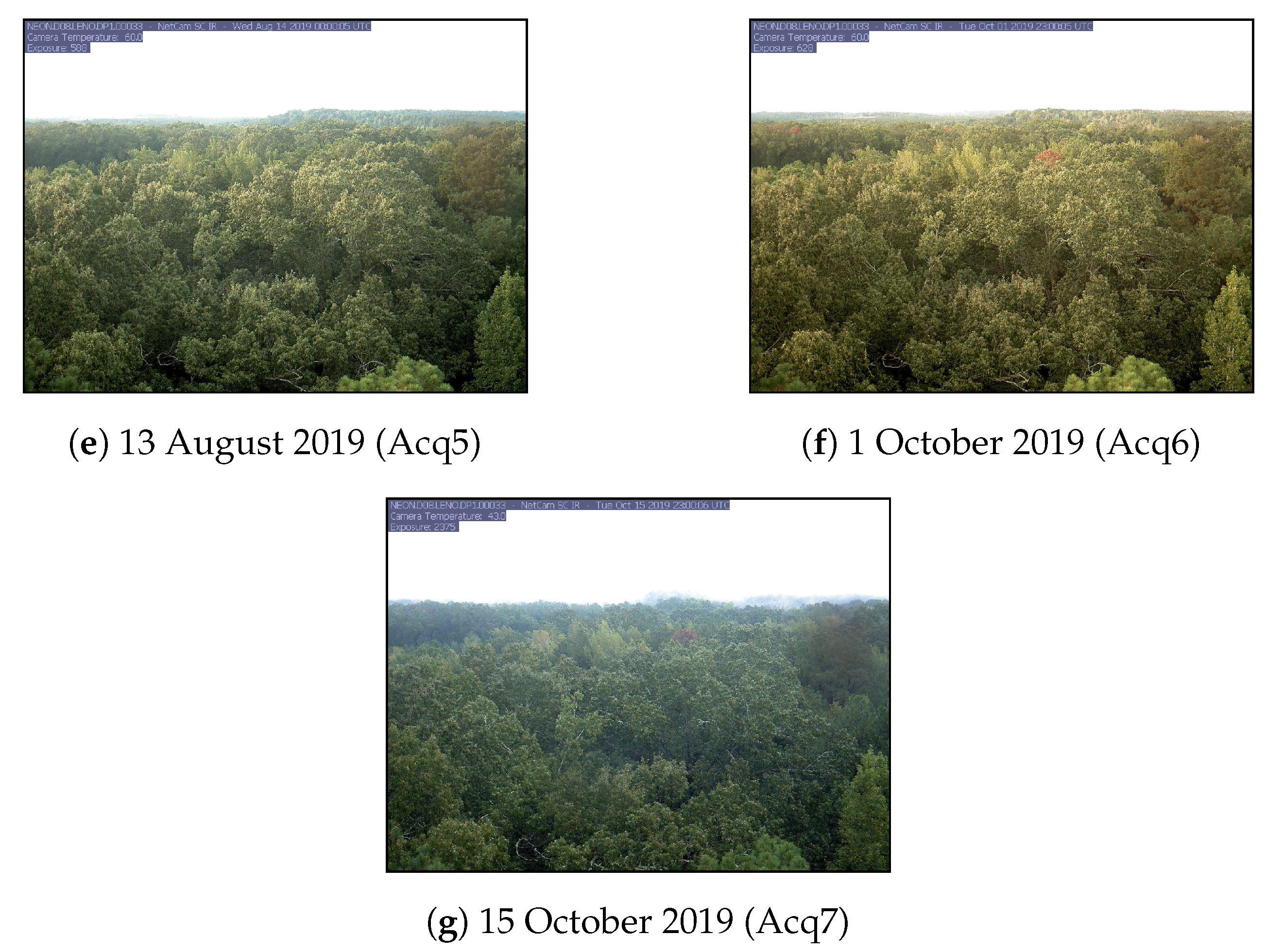
2.1. Study Site and Field Survey

The Lenoir Landing site part of the Choctaw National Wildlife Refuge (31.85388 N, 88.16122 W) is located in southwest Alabama along the Tombigbee River and features a temperate deciduous forest. The site has deciduous hardwood trees and woody wetlands prone to seasonal flooding each spring. The mean elevation of the site is 20 m above mean sea level. The dominant tree species are American sweetgum (Liquidambar styraciflua), American hornbeam (Carpinus caroliniana), and loblolly pine (Pinus taeda). Extensive field survey was carried out under the National Ecological Observatory Network (NEON) [33] to collect parameters such as tree DBH (diameter at breast height or 1.3 m above ground), species, and tree height. 41 plots measuring 20 m × 20 m (0.04 ha) have been surveyed between 2015 to 2019. Additionally, ten plots measuring 40 m × 40 m are surveyed in November 2019. The 5484 trees surveyed in these plots can be grouped according to species-groups listed by Jenkins et al. [34] as hardwood, woodland, and softwood. The distribution of these tree species-groups in the surveyed plots is hardwood species (71%), woodland species (11%), softwood species including conifers (2%) while the remaining are shrubs or are unclassified. The national land-cover database (NLCD) 2016 released by multi-resolution land characteristics consortium (MRLC) is also used to identify the major vegetation type for the plot. 54.5% of plots are in woody wetlands, 29% are in deciduous forests, 12% are in mixed forest while the remaining plots are in shrub/scrub forested areas. The geolocation of the plot corners is accurately determined using a dual-frequency GPS receiver. The DBH is measured for all trees with DBH greater than 2.5 cm. The height of a few trees in each plot is also measured. The DBH measured for each tree is converted to growing stock volume (GSV) and biomass using species-specific allometric equations and wood-specific density [34]. The aggregated plot-level AGB ranges between 0.05 Mg/ha to 373 Mg/ha with a mean AGB of 157 Mg/ha.
A permanent flux tower and network of soil moisture sensors near the flux tower measure precipitation, temperature, and volumetric soil water content or soil moisture (cm3/cm3) at 0.01 m below the ground. The location of the field plots and the flux tower is shown in Figure 1, and the measured soil moisture and cumulative precipitation before each acquisition is shown in Table 1. The flux tower also has a phenology camera that captures images of the canopy at 15 min intervals. Figure 2 shows the images captured around one hour before the UAVSAR acquisition.

2.2. Lidar Data and Reference AGB Map

A reference AGB map is generated from small-footprint LIDAR-derived canopy height to mitigate errors that would result from calibrating SAR-AGB relationships directly with small plots [4]. Canopy height in meters above the bare Earth is generated at 1 m resolution using small footprint LIDAR data collected from NEON Airborne Observation Platform (AOP) LIDAR—Optech LIDAR Gemini instrument [33]. The plot-level AGB is related to LIDAR measured canopy height using a least-squares minimization regression fit using a power function [35]. This provides a reference AGB map at 1 m posting resampled to the UAVSAR SLC data in slant range. The reference AGB map generated using LIDAR data has RMSE of 17.5 Mg/ha for AGB less than 100 Mg/ha. The RMSE for higher AGB (up to 335 Mg/ha) regions is 48 Mg/ha. The extrapolation of field AGB to LIDAR provides wider spatial coverage and higher training samples [3]. 311 random samples (referred to as polygons) of approximately 1 ha are selected in the test site. Figure 1 shows the LIDAR height map and the surveyed 0.04 ha plots and LIDAR-upscaled 1 ha polygons. The AGB for these 311 polygons varies from 1.8 Mg/ha to 335 Mg/ha with a mean of 125 Mg/ha. The major NLCD forest-types represented by these 1 ha polygons are woody wetlands (43%), evergreen forests (26%), and mixed and deciduous forests (15%) while the remaining polygons are in scrub and herbaceous forests. Among these 311 polygons, 24 polygons (8%) are excluded from the analysis as these partially cover non-forest regions including roads and water-bodies.

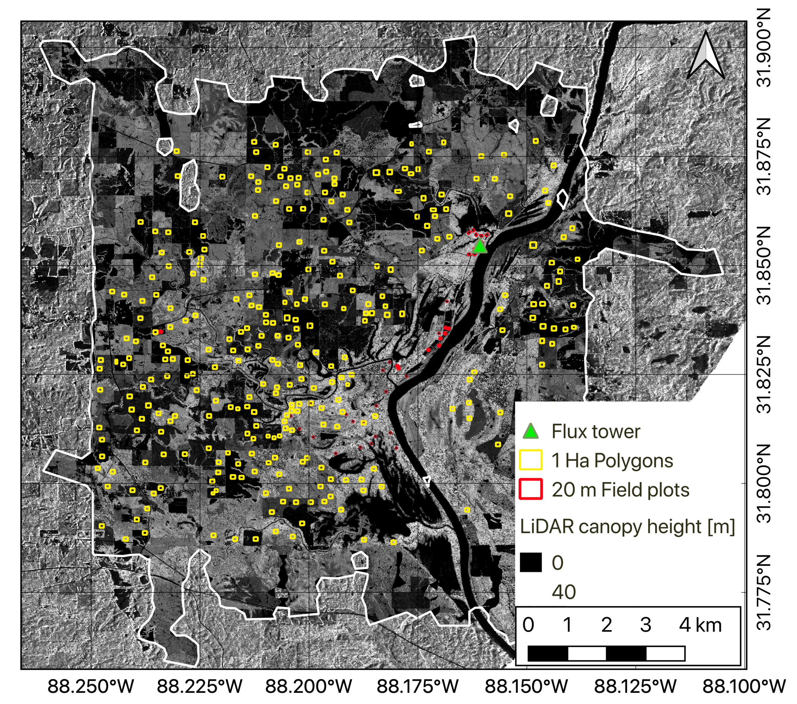
2.3. AM-PM Campaign SAR Data

A total of seven L-band SAR acquisitions were collected over the Lenoir Landing forest site between 6 June to 15 October 2019 as part of the UAVSAR AM-PM campaign. The SAR backscatter for these data are collected under different acquisition conditions (soil moisture and precipitation) as detailed in Table 1. The data on October, 1 (Acq6) is acquired under dry conditions with no precipitation in the preceding 72 h (hours) and a very low soil moisture of 0.08 cm3/cm3 or 8%. On the other hand, the data on October, 15 (Acq7) can be considered as a case of very wet acquisition as it was acquired during a precipitation event and a very high soil moisture of 0.48 cm3/cm3. Note that 0 h precipitation denotes rainfall measured during the approximately 5 min of acquisition time of the UAVSAR flight.
The UAVSAR data are acquired at 6-pm local time to match the NISAR ascending pass. The look angle of UAVSAR varies from 21° in near range to 65° in far range. However, the field plots and 1 ha polygons cover a smaller incidence angle range of 34° to 50°. The data are provided as SLC with azimuth resolution of 0.6 m and range resolution coarser than 1.87 m. Here, we examine the cross-polarimetric (HV) channel that is relevant to biomass estimation from systematic dual-polarimetric SAR missions like ALOS-2 and NISAR.
The UAVSAR data is radiometrically calibrated and co-registered using the 1-arc second SRTM DEM to form a stack of seven SLC images. The SLC images store radar backscatter as σ 0 (referenced to the flat ellipsoid), which is modulated by topography. An improved radiometric terrain correction (RTC) algorithm [36] is applied to flatten the backscatter and generate γ 0 . Our approach for RTC includes compensation of backscatter variation due to changing radar look angle across the imaged swath. The algorithm generates a flattened backscatter image ideally free of radiometric modulations caused by topography and incidence angle variations. In the RTC process, the plot corners are projected to radar geometry, and sub-pixel aggregation of backscatter is carried out. Further, this aggregation approach ensures that there is no mismatch between pixel size and plot size, as even partially covered pixels are weighted according to their areal coverage. The 1-ha backscatter averaging reduces noise and speckle from the full resolution SAR data.

3. Methodology

The 3-parameter Water Cloud Model (WCM) [37] is adopted in this research to estimate the forest AGB. The WCM model is a physically-based model that presents the SAR backscatter as a function of forest biophysical parameters. For modeling L-band SAR backscatter, a version of WCM is used which accounts for vertical and horizontal discontinuities or gaps in the forest canopy [38,39]. The WCM model is selected as it has a strong physical foundation as shown in [37,38,39] and has been used to map forest biomass from L-band backscatter in numerous studies [2,22,24,40]. In addition, the NISAR and BIOMASS missions are planning their cal/val and biomass mapping activities on models based on WCM given its simplistic form and wide applicability.
The WCM model expresses backscatter as the incoherent sum of ground (parameter a) and vegetation (parameter b) scattering contributions weighted by the attenuation due to a vegetation layer (factor e c β )
γ 0 = a e c β + b ( 1 e c β )
where β is the above-ground biomass in Mg/ha. The derivation of (1) is not discussed here as it has been extensively discussed by [38,39]. The model parameters a, b, and c are estimated from SAR and lidar-based AGB map data after applying a χ -squared minimization approach using 137 1-ha polygons with AGB up to 100 Mg/ha.

3.1. Model Calibration and Validation

To analyze the impact of varying acquisition conditions, and the utility of multi-temporal data to reduce the AGB estimation errors, we consider the following distinct cases:
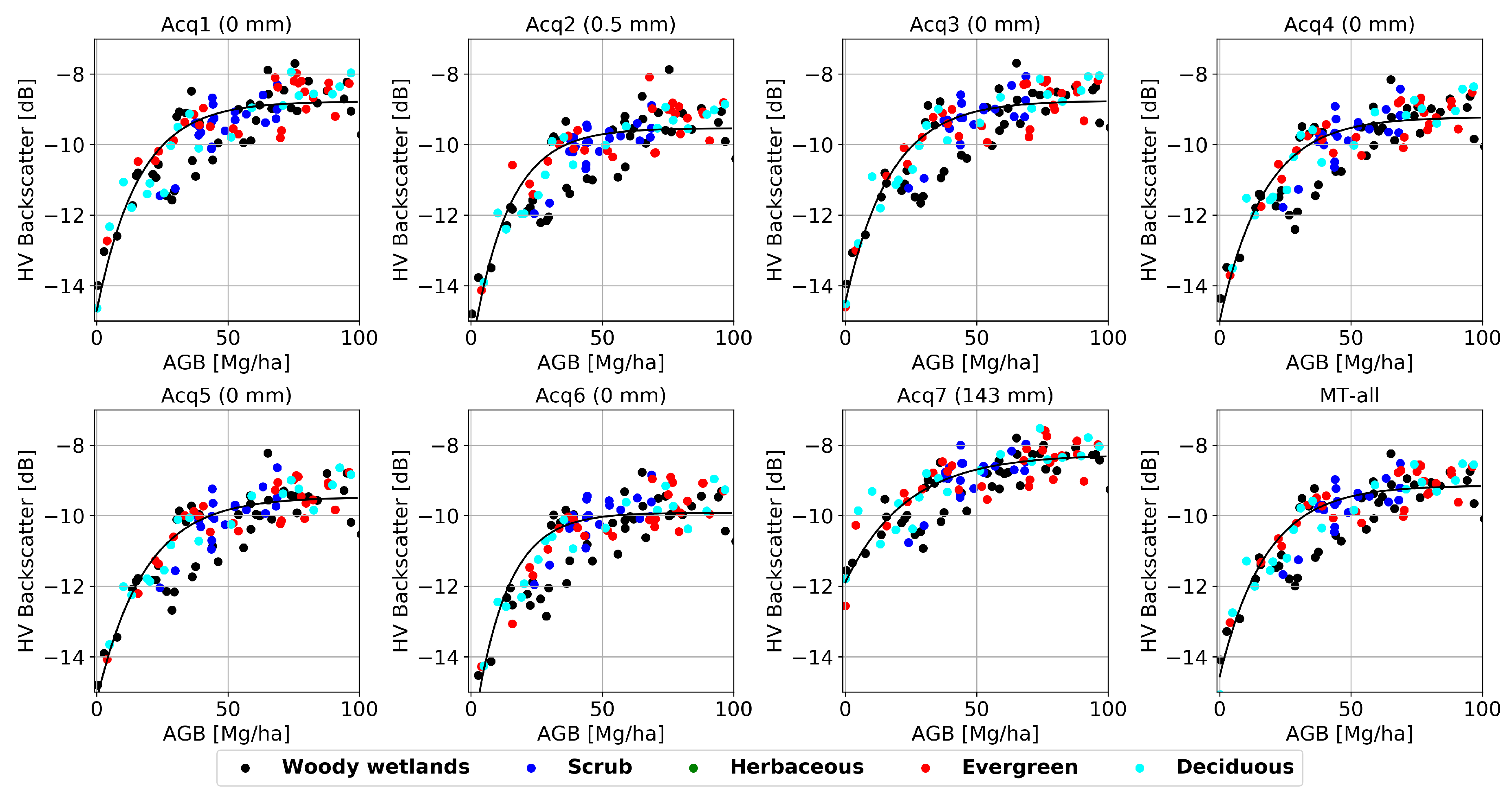
  • Single acquisition backscatter: The model is trained and validated using the seven L-band cross-polarized backscatter with different acquisition conditions (case 1).
  • Multi-temporal averaged backscatter: The temporal mean of HV backscatter over all the seven acquisitions (MT-all, case 2) and the temporal mean of HV backscatter over acquisitions without rainfall in the 24 h preceding the acquisition time (MT-24, case 3)
  • The multi-temporal weighted average (WA) of AGB is estimated from the seven acquisitions (case 4) with the weights explained below.
Case 1 addresses the first objective (see Section 1) of this study, while the other three cases (case 2–case 4) address the second objective and explore the ability of multi-temporal data to improve the AGB estimation performance. For the first three cases, the backscatter is modeled to estimate AGB, while for case 4, the modeled AGB from case 1 is the input to estimate the weighted average AGB. Hence, the WCM model parameters are reported for the first three cases.
To map AGB for the first three cases, the WCM model is calibrated using 60% randomly-selected polygons and validated over the remaining 40% polygons. The calibration and validation process is iterated 30 times with the data split randomly into training and test sets to allow robust estimation of the error. The WCM model is calibrated for each case by estimating the model parameters a, b and c. The root mean squared deviation (RMSD), coefficient of determination ( R 2 ), saturation level, and number of valid solutions are used to compare the performance obtained for each case. The backscatter saturation level β s a t for a given WCM model is obtained by deriving the value of biomass that gives a change in backscatter due to speckle equal to the backscatter associated with the desired biomass error (20 Mg/ha according to the NISAR requirements) [19]. For a WCM model characterized by parameters a, b and c, solving (1) for β = β s a t provides the backscatter ( γ s a t 0 ) at which the WCM curve saturates. The valid solution space is the region between the modeled backscatter values ranging from a to γ s a t 0 . In case a polygon has backscatter outside this valid range [39] a biomass value is assigned. Polygons with backscatter lower than the ground scattering component a are assumed to have 0 Mg/ha biomass and polygons with backscatter higher than γ s a t 0 are assigned the maximum AGB.
Multi-temporal data stack can improve the AGB retrieval results using a weighted combination of the AGB estimated from individual acquisitions as shown by [2,13,23,24,39]. The multi-temporal biomass, β m t is computed for a particular polygon from a weighted combination of biomass estimates ( β i ) from the seven acquisitions as:
β m t = i = 1 N w i β i i = 1 N w i
The weights w i are calculated using two approaches (1) the difference between the parameters a and b, i.e., the dynamic range between backscatter from the ground and from the forest with infinite biomass (WA-DR); (2) the inverse of the soil moisture measured for each acquisition (WA-SM).

3.2. Temporal Cross-Validation of the Model

The robustness of the model trained and validated under different acquisition conditions is analyzed by considering the scenario of calibrating the model from each of the first three cases and validating it with all the other cases. The WCM model parameters (a, b, and c) obtained for each of the first three cases listed above are applied to randomly-selected 80% polygons in the remaining cases to generate all cross-cases combinations of calibration and validation of the AGB. This means, for instance, that the model generated for one date (Acq 1) is evaluated on other dates (Acq2–Acq7) and the multi-temporal mean backscatter (MT-all and MT-24). This step is iterated 30 times with randomly selected validation polygons to provide a robust estimate of cross-validation and model stability.

4. Results and Discussion

4.1. Analysis of Backscatter versus Biomass

The variation of backscatter with respect to forest AGB is analyzed as a function of forest type and with acquisition conditions such as precipitation and soil moisture. Figure 3 shows the HV backscatter and the WCM model curves as a function of AGB for all 7 individual acquisitions (case 1 in Section 3.1) along with the mean backscatter for all the seven acquisitions (case 2 in Section 3.1). The SAR backscatter increases with increasing forest AGB, especially for low forest biomass. Overall, for the seven acquisitions, the SAR backscatter-AGB trends agree with previous L-band analysis reported in temperate as well as other forest environments [21,23,41,42,43,44,45,46,47]. Observation taken during significant rainfall event (Acq7) showed increased backscatter and lower dynamic range.
SAR backscatter magnitude changes with the dielectric constant as well as the surface roughness [48,49,50,51]. For a polygon representing a forested region, the backscatter varies over the seven acquisitions due to changes in soil moisture and precipitation. Overall, the backscatter increases for acquisitions during precipitation (Acq7) or with higher soil moisture (Acq1). Similarly, acquisitions with dry soil conditions (Acq6) have lower backscatter. Mean backscatter for Acq7 with wet soil conditions (0.48 cm3/cm3) is −9.2 dB ± 1.5 dB, whereas for Acq6 with dry soil conditions (0.08 cm3/cm3) it is about 2 dB lower (−11.1 dB ± 2.3 dB). The backscatter variation is also dependent on the forest AGB. The impact of precipitation and soil moisture is particularly visible in the low AGB range, where the WCM curve of Acq7 lies about 2 to 5 dB higher than the WCM curve of Acq6. The variation in backscatter is caused by the change in soil permittivity as a result of increased soil moisture. This is consistent with higher sensitivity for low AGB regions reported for tropical [27] and boreal forests [8].
The WCM model curves show that the model adapts to the variation in the backscatter in response to soil moisture or precipitation changes. We attempt to evaluate whether this backscatter change is influenced by the major forest-type of the polygons. The polygons covering herbaceous forests (see Figure 3) have low AGB (up to 20 Mg/ha) and the backscatter is more sensitive to soil moisture and precipitation due to sparser canopy cover. For Acq7, the backscatter for these herbaceous forests is about 2.23 dB lower. Polygons dominated by deciduous and mixed forests have AGB varying between 20 Mg/ha and 100 Mg/ha. These polygons show a uniform 1 dB decrease in backscatter for Acq7 and this decrease is uniform across the AGB range. The polygons dominated by woody wetlands also cover an AGB range between 20 Mg/ha and 100 Mg/ha. However, for Acq7 the backscatter decreases by almost 2 dB for low AGB (<20 Mg/ha) polygons and by 0.75 dB for polygons with AGB above 40 Mg/ha. This higher sensitivity of backscatter to lower AGB polygons is explained by the presence of wet soil or water in the woody wetlands and lower canopy density.

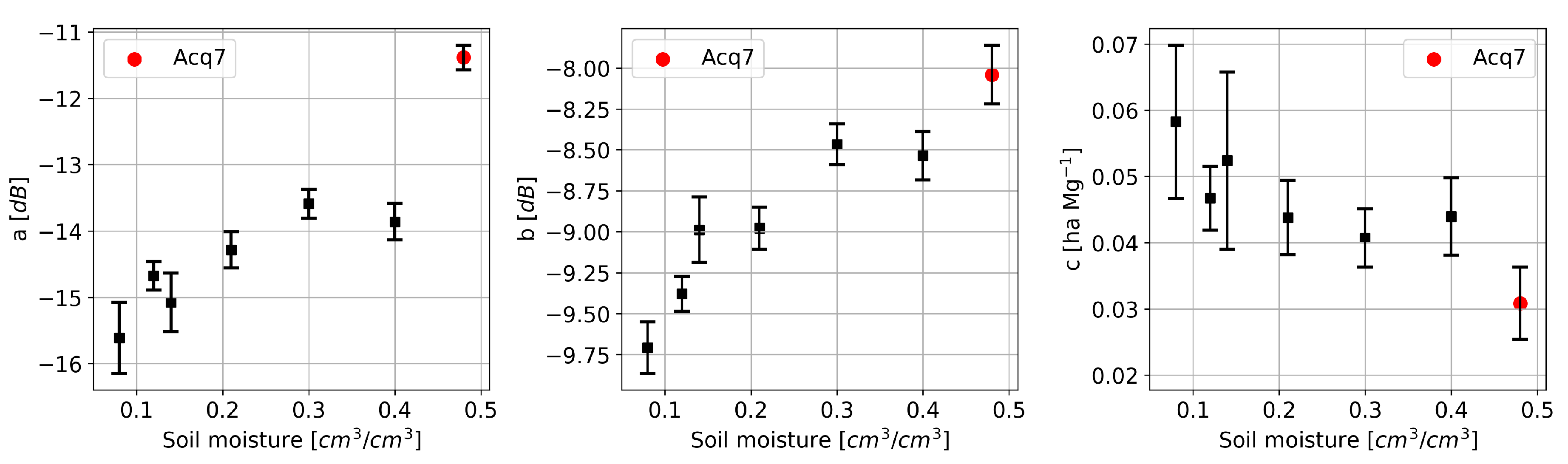
4.2. Estimates of WCM Parameters

Model training on the first three cases explained in Section 3.1 was carried out by estimating the WCM parameters a, b and c with a χ -squared minimization approach. Figure 4 shows the variation of WCM parameters with soil moisture for case 1. Parameters a, b and c represent the ground and canopy scattering contribution and the microwave extinction due to vegetation, respectively. Overall, with the increase in soil moisture, parameters a and b increase while c decreases. The parameters a and b are positively correlated with soil moisture having a correlation of 0.88 ( p < 0.05 ) and 0.96 ( p < 0.05 ), respectively. The parameter c is negatively correlated with soil moisture ( r = 0.71 ), however, the correlation is not statistically significant within the 95% confidence interval with p = 0.07 . Compared to other acquisitions, an additional increase in parameters a and b and a decrease in parameter c is observed for Acq7. This is attributed to high precipitation measured during the acquisition. The increase is highest in a with a 5 dB excursion from dry to wet conditions. This is expected as a represents the scattering contribution from the ground, and therefore it is more sensitive to changes in soil water content. The dynamic range of the WCM model decreases from 6 dB to 5 dB with an increase in soil moisture from 0.08 cm3/cm3 to 0.40 cm3/cm3. This reduction in dynamic range translates into smaller signal attenuation in the canopy modeled by the WCM model (parameter c). The dynamic range is a measure of the sensitivity of the backscatter to forest AGB [52]. Interestingly, for Acq7, the dynamic range of the WCM model reduces to 3.5 dB which shows the impact of precipitation in addition to soil moisture increase. As seen in Figure 3, the impact of precipitation on Acq7 backscatter is higher for low AGB polygons and reduces as AGB increases. Therefore, precipitation appears to reduce the range of the backscatter measured over the polygons and the WCM model’s dynamic range. The effect of these variations in WCM parameters on the estimated AGB is analyzed in the next section.

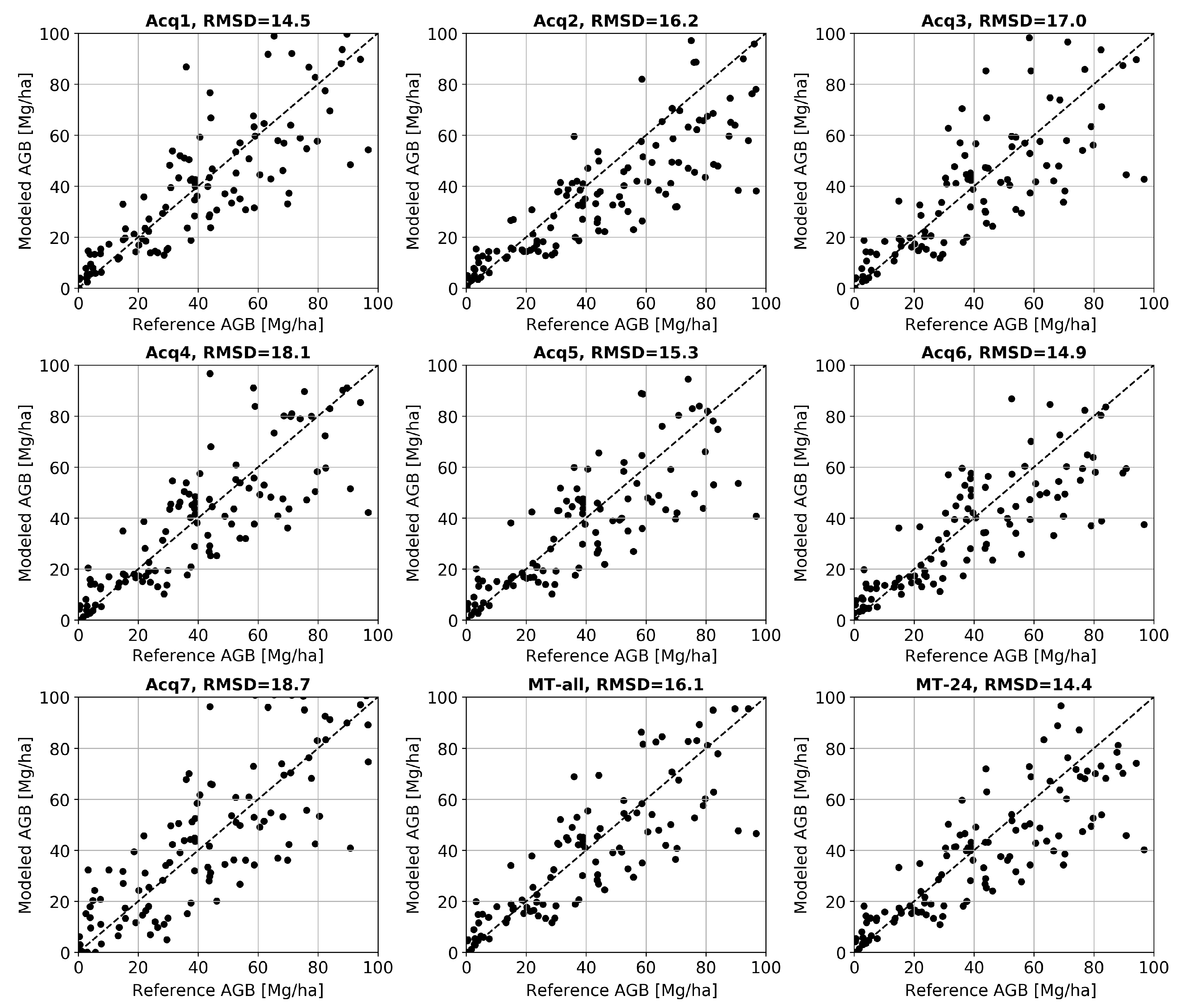
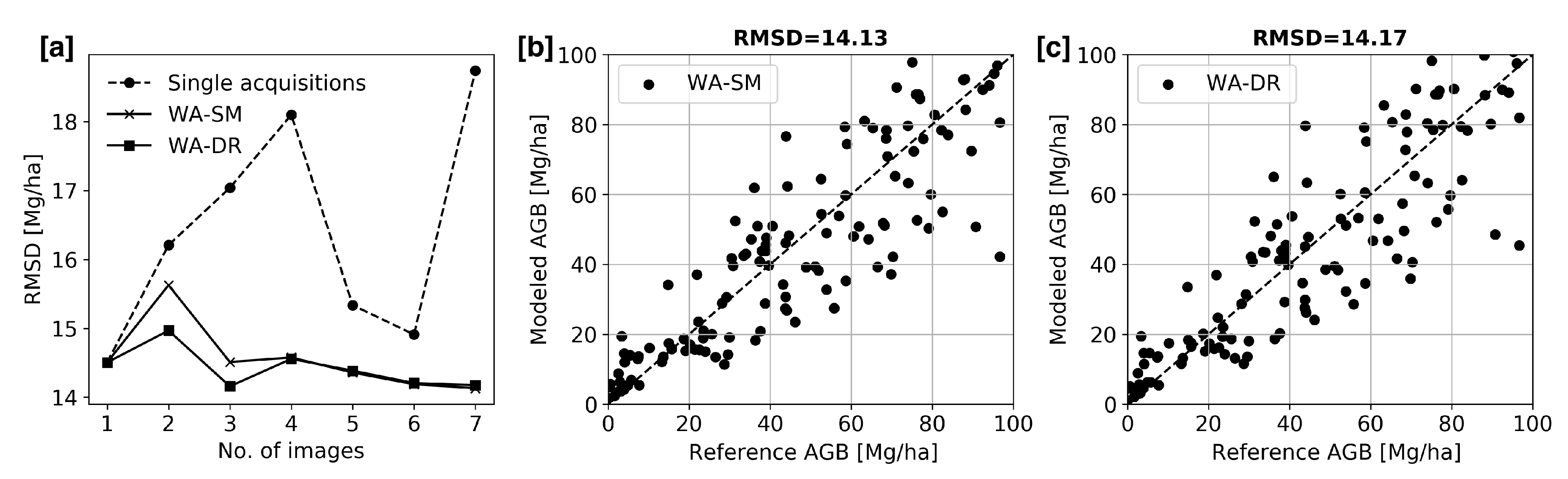
4.3. AGB Retrieval Performance

The estimated WCM parameters are used to invert the WCM model and estimate the forest AGB. The section first analyzes the AGB retrieval performance using single acquisitions (case 1) followed by multi-temporal average backscatter (case 2 and case 3) and multi-temporal weighted average of AGB (case 4). The AGB co-validation of models calibrated and validated for each backscatter case of Section 3.1 is shown in Table 2. The corresponding validation scatter-plots between the LIDAR AGB and WCM modeled AGB are shown in Figure 5. The figure clearly shows that the AGB retrieval performance varies for each acquisition. At 1 ha scale, AGB estimation from single acquisitions (case 1) leads to RMS deviation with respect to LIDAR AGB between 14.5 Mg/ha and 18.7 Mg/ha. Data acquired during precipitation and wet soil conditions (Acq7) has the highest error with RMSD of 18.7 Mg/ha. With multi-temporal average backscatter, the RMSD is 16.1 Mg/ha (MT-all, case 2) and further reduces to 14.4 Mg/ha (MT-24, case 3). From Figure 4 and Figure 5, it is observed that the dynamic range of the WCM model is related to the soil moisture and a lower dynamic range results in higher RMSD. These results are consistent with previous findings [2,47]. Excluding acquisitions with precipitation (MT-24) reduces the backscatter variations and improves the AGB estimate by 12% compared to the mean RMSD of individual acquisitions.
Figure 6 illustrates the advantage of having multi-temporal AGB estimates. The dashed line shows the RMSD for all seven single acquisitions (case 1) while the solid lines represent the improvement in RMSD when each acquisition is successively added to the multi-temporal weighted average. The multi-temporal weighted average of the AGB estimates from all seven acquisitions in case 1, weighted by the inverse of the soil moisture (WA-SM) or by the dynamic range (WA-DR) have higher accuracy with RMSD of 14.13 Mg/ha and 14.17 Mg/ha respectively. Although both the parameters used as weights for averaging result in the similar performance, it is important to note the advantage of using dynamic range over regions where soil moisture products are not available at sufficient temporal or spatial resolutions.
It is important to also discuss the impact of multi-temporal weighted average AGB estimates on valid solution range. As discussed in Section 3, the polygons with backscatter outside the range defined by parameter a and b are assigned an AGB value of either 0 Mg/ha or maximum biomass. However, this adds further uncertainty in AGB estimates as the true value of AGB is not known. The percentage of polygons with backscatter outside the dynamic range for each of the above cases is computed. It is observed that the weighted average AGB estimates have the least number of polygons outside the dynamic range (7%) while the corresponding values for single acquisition ranges between 24% to 16%. This demonstrates the impact of varying acquisition conditions on AGB estimation and the advantage of multi-temporal acquisitions.

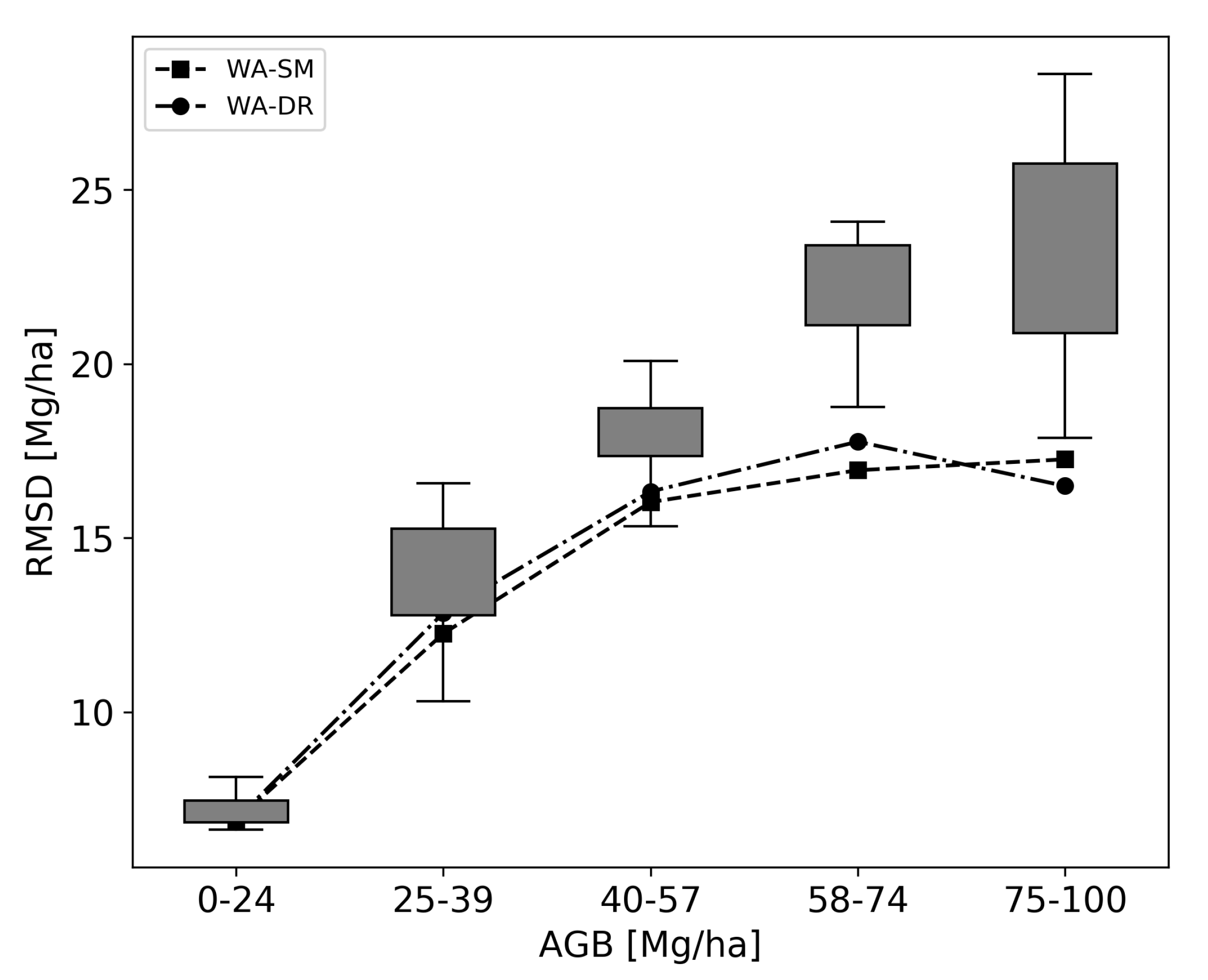
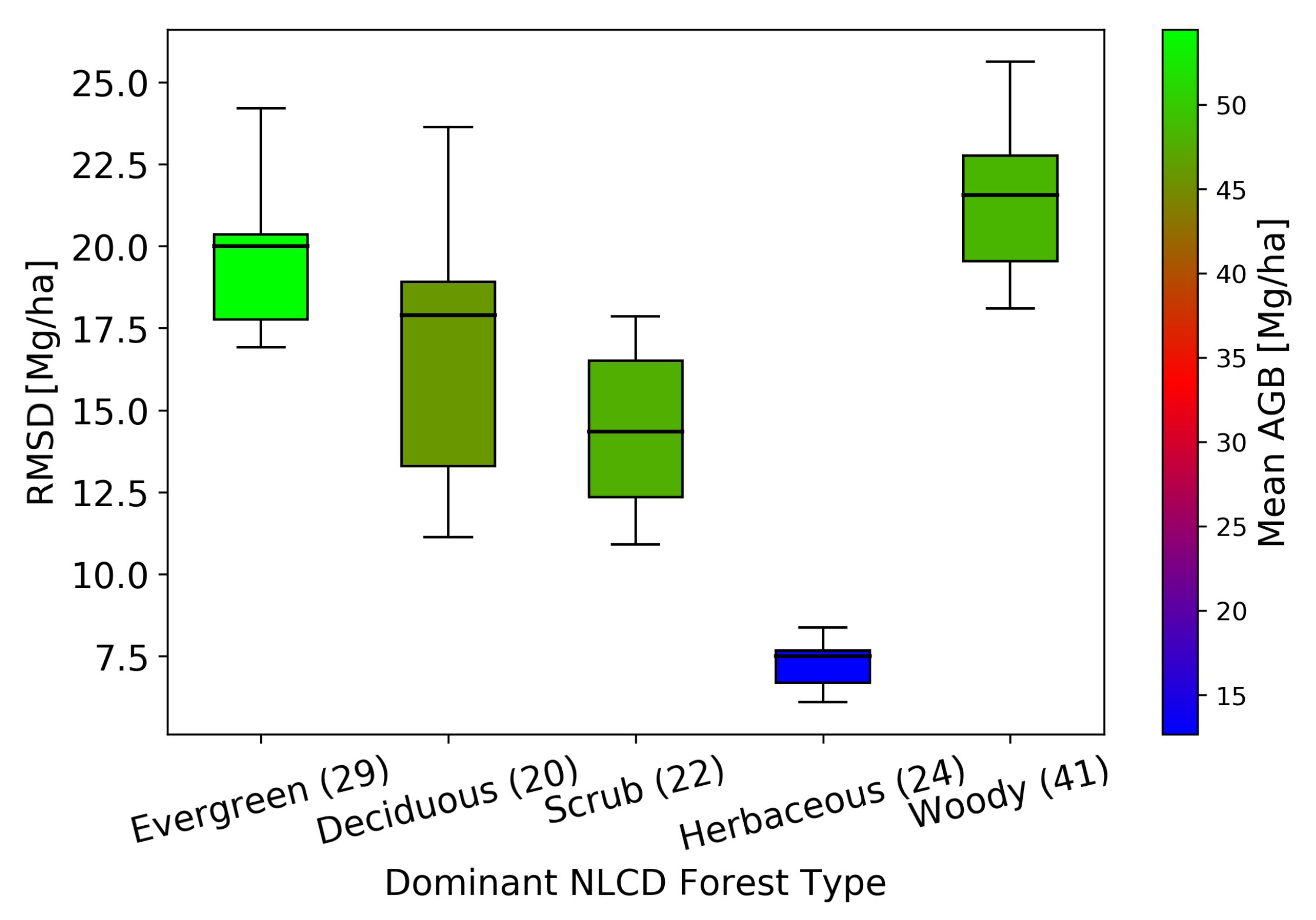
4.4. Factors Influencing AGB Retrieval

SAR backscatter is influenced by (1) forest structural parameters including forest density, tree species, shape of canopy, and (2) environmental parameters including soil moisture and precipitation [22]. Conifers and deciduous species have distinct canopy shape. However, the Lenoir Landing site is dominated by hardwood and woodland species with a small proportion (2%) of the 0.04 Ha plots dominated with coniferous species (see Section 2.1). The effect of acquisition conditions (soil moisture and precipitation) on WCM modeling parameters and AGB retrieval are discussed earlier. The accuracy of AGB retrieval across different AGB regions and for different NLCD forest types are analyzed in this section.

4.4.1. AGB Range or Density of Forest

Figure 7 shows the AGB inversion RMSD box-plots (mean, quantiles, and minimum and maximum RMSD values) for the seven single acquisitions over five AGB ranges. The AGB class boundary is selected such that equal sampling of polygons is possible across all regions. The dashed and dash-dotted lines show the RMSD for the weighted average RMSD. The advantage of having multi-temporal acquisitions and using a weighted average RMSD can be appreciated. The RMSD increases with AGB and stabilizes around a mean of 22.5 Mg/ha for case 1. With WA-SM and WA-DR, the RMSD is much lower at 17 Mg/ha which shows a significant improvement in AGB retrieval performance over single-acquisitions.

4.4.2. NLCD Forest Type

The NLCD provides a broad perspective regarding the major forest canopy type within the study area. Figure 8 shows the box plot of the RMSD for the seven acquisitions over five major NLCD classes. The colors represent the mean AGB for each NLCD class. Forests in all the major NLCD classes have RMSD below 25 Mg/ha with the woody wetlands having a higher deviation in AGB retrieval. This might be due to the presence of under-canopy wet soil not accurately modeled by the WCM model. The low-AGB forests (grassland NLCD class) have a relatively higher RMSD compared to their mean AGB. In these low-AGB regions, the changes in ground characteristics have a higher impact on SAR backscatter leading to higher RMSD.

4.5. Temporal AGB Cross-Validation

The RMSD from all cross-validation cases are computed and shown by the box-plot in Figure 9. For Acq7, cross-validation leads to the highest RMSD as backscatter is affected by precipitation. The cross-validation RMSD ranges between 22 and 33 Mg/ha in contrast to the co-validation RMSD of 18.70 Mg/ha. This shows that due caution is needed when applying models trained under wet acquisition conditions across multiple acquisitions. The model trained with Acq6 resulted in invalid solutions for about 60 % of cross-validation samples due to saturation of the backscatter-AGB curve. This suggests that the valid inversion backscatter interval needs to be considered for cross-validation. Backscatter does not increase significantly for biomass values beyond the saturation level β s a t (see Figure 3). γ s a t 0 is the backscatter at which the WCM curve saturates (see Section 3.1) and provides the upper limit of backscatter that can be inverted within a pre-defined error limit using the WCM model. This is important for cross-validation as the backscatter can vary between acquisitions due to changes in environmental conditions as shown in this analysis. The WCM curve saturates at −8.0 dB for acquisition with wet soil conditions (Acq7, see Figure 3) and at −9.8 dB for acquisition with dry soil conditions (Acq6). This implies that when the model calibrated using Acq6 is validated over other backscatter cases, all polygons with backscatter higher than −9.8 dB will not result in a valid solution. The percentage of polygons with valid solutions is shown by the color gradient in Figure 9.

4.6. Limitations of the Study

The results presented in this section show the impact of dry and wet acquisition conditions on AGB estimation performance and the advantage of multi-temporal data to mitigate this impact. It is essential to discuss a few limitations related to the data and methodology.
First, as mentioned in Section 3.1, we use data acquired during dry and wet imaging conditions. These conditions are assessed from precipitation and soil moisture measurements available from one location (flux tower). The conditions can deviate locally from those observed at the flux tower. However, as these measuring sensors are within the forest site, the spatial variability is reduced.
When using multiple SAR acquisitions, bias can be introduced due to temporal changes in forest or soil. In this study, this is minimized as all the acquisitions are collected within the summer and beginning of fall 2019. As no acquisitions are collected during the spring season when flooding occurs, the impact of standing water on the backscatter-AGB relationship is not analyzed in this paper. Extending this analysis with multi-temporal SAR data acquired through all seasons would provide a more extensive data-set to capture the combined impact of weather and seasonal changes (leaf on/off) on backscatter-AGB relation. The NISAR mission will provide dense time-series similar to the one used in this analysis, capable of generating multiple acquisitions over different seasons or growth cycles unique to each forest eco-region. This analysis is limited to forests with AGB less than 100 Mg/ha in agreement with the upper limit established by the NISAR mission science requirements.
The reported AGB accuracy does not include errors from field-estimated and LIDAR-derived AGB, which may be caused by uncertainties in allometry, geolocation, and relation between LIDAR Canopy Height Model (CHM) and field AGB. Chave [29] reported errors of 5% for allometric equations over tropical forests with field plots of 1 ha. This error is expected to be higher for smaller field plots. The GPS geolocation uncertainty for NEON field plots is below 1 m. For the small plot size (0.04 ha), this can lead to errors in highly heterogeneous forests when the field AGB is used to generate LIDAR AGB maps. For the Lenoir Landing site, the forest in most field plots is homogeneous, so we expect this error to be minimal.
Furthermore, the inherent difference in viewing geometry of LIDAR and SAR will impact the accuracy of LIDAR AGB-SAR backscatter relationship when LIDAR AGB is projected to slant-range geometry. The airborne geometry, motion compensation and processing may introduce small artifacts in the data. The accuracy of reference LIDAR AGB depends on the ability of field plots to represent the species diversity within the study site. For forests with higher heterogeneity within plots, the intra-plot tree-density distribution would lead to a higher variance of observed backscatter for similar AGB values. This leads to a larger variance in model coefficients and higher error in AGB estimates. These errors, however, do not affect the conclusions drawn from this analysis. To obtain an absolute AGB accuracy, propagation of errors, which is out of the scope of this paper, should be carried out [4,19].

5. Conclusions

This study reports quantitatively the impact of backscatter perturbations due to changes in acquisition conditions on AGB estimation performance over a temperate broadleaf forest using new airborne campaign data acquired during the 2019 UAVSAR AM-PM Campaign. The advantage of using multi-temporal data to reduce the AGB estimation errors is also assessed and confirmed in the context of upcoming SAR missions. Precipitation affects AGB retrieval accuracy with up to 20% increase in AGB estimation errors. The WCM model parameters are highly correlated with measured soil moisture with correlation (r) of 0.88 and 0.96 for parameters a and b, respectively. Furthermore, soil moisture changes do not significantly affect the co-validation AGB estimation accuracy. Models calibrated and validated using acquisitions with significantly different meteorological conditions provide erroneous AGB estimates, with the RMSD increasing by up to a factor of 2 compared with co-validation RMSD. This emphasizes the challenges of calibrating backscatter-AGB models coping with soil moisture changes and precipitation and expected to be valid over multiple acquisitions in a time-series. This is evident in the temporal cross-validation analysis shown in this study. Capitalizing on the time-series data, we used the weighted average of the AGB estimated from multiple acquisitions weighted by the dynamic range and soil moisture to reduce the impact of changing acquisition conditions. The analysis can be further expanded over other forest eco-regions and with the use of a denser SAR time-series data-set.

Author Contributions

Conceptualization, U.K. and M.L.; methodology, U.K. and M.L.; software, M.L. and G.H.X.S.; validation, U.K. and V.M.; formal analysis, U.K.; investigation, U.K. and M.L.; resources, M.L. and B.C.; data curation, U.K.; writing—original draft preparation, U.K. and M.L.; writing—review and editing, G.H.X.S. and V.M.; visualization, U.K.; supervision, M.L.; project administration, M.L.; funding acquisition, M.L. and B.C. All authors have read and agreed to the published version of the manuscript.

Funding

This work was conducted at the Jet Propulsion Laboratory, California Institute of Technology, under contract with NASA as part of the NISAR Project Science Team activities.

Acknowledgments

The authors would like to thank the UAVSAR and NISAR teams for designing the AM-PM Campaign and making the single-look complex SAR data available. A prototype of this work was developed and tested on the pilot version of the joint NASA-ESA Multi-Mission Algorithm and Analysis Platform (MAAP). The authors would like to thank the MAAP team for the technical support. The authors thank the NISAR Project and Algorithm Definition Team (ADT) for providing the InSAR Scientific Computing Environment (ISCE3) software that was used for co-registering and radiometric-terrain correcting the UAVSAR SLC stack. The authors thank the National Ecological Observatory Network (NEON) Program for the field, LIDAR, and meteorological data acquired over the study site.

Conflicts of Interest

The authors declare no conflict of interest.

References

  1. Santoro, M.; Cartus, O. Research Pathways of Forest Above-Ground Biomass Estimation Based on SAR Backscatter and Interferometric SAR Observations. Remote Sens. 2018, 10, 608. [Google Scholar] [CrossRef] [Green Version]
  2. Cartus, O.; Santoro, M.; Kellndorfer, J. Mapping forest aboveground biomass in the Northeastern United States with ALOS PALSAR dual-polarization L-band. Remote Sens. Environ. 2012, 124, 466–478. [Google Scholar] [CrossRef]
  3. Tanase, M.A.; Panciera, R.; Lowell, K.; Tian, S.; Hacker, J.M.; Walker, J.P. Airborne multi-temporal L-band polarimetric SAR data for biomass estimation in semi-arid forests. Remote Sens. Environ. 2014, 145, 93–104. [Google Scholar] [CrossRef]
  4. Bouvet, A.; Mermoz, S.; Le Toan, T.; Villard, L.; Mathieu, R.; Naidoo, L.; Asner, G.P. An above-ground biomass map of African savannahs and woodlands at 25 m resolution derived from ALOS PALSAR. Remote Sens. Environ. 2018, 206, 156–173. [Google Scholar] [CrossRef]
  5. Yu, Y.; Saatchi, S. Sensitivity of L-Band SAR Backscatter to Aboveground Biomass of Global Forests. Remote Sens. 2016, 8, 522. [Google Scholar] [CrossRef] [Green Version]
  6. Luckman, A.; Baker, J.; Kuplich, T.M.; Yanasse, C.d.C.F.; Frery, A. A study of the relationship between radar backscatter and regenerating tropical forest biomass for Spaceborne SAR Instruments. Remote Sens. Environ. 1997, 60, 1–13. [Google Scholar] [CrossRef]
  7. Luckman, A.; Baker, J.; Honzák, M.; Lucas, R. Tropical Forest Biomass Density Estimation Using JERS-1 SAR: Seasonal Variation, Confidence Limits, and Application to Image Mosaics. Remote Sens. Environ. 1998, 63, 126–139. [Google Scholar] [CrossRef]
  8. Salas, W.A.; Ducey, M.J.; Rignot, E.; Skole, D. Assessment of JERS-1 SAR for monitoring secondary vegetation in Amazonia: I. Spatial and temporal variability in backscatter across a chrono-sequence of secondary vegetation stands in Rondonia. Int. J. Remote Sens. 2002, 23, 1357–1379. [Google Scholar] [CrossRef]
  9. Takeuchi, S.; Suga, Y.; Oguro, Y.; Konishi, T. Monitoring of new plantation development in tropical rain forests using JERS-1 SAR data. Adv. Space Res. 2000, 26, 1151–1154. [Google Scholar] [CrossRef]
  10. Kasischke, E.S.; Melack, J.M.; Craig Dobson, M. The use of imaging radars for ecological applications—A review. Remote Sens. Environ. 1997, 59, 141–156. [Google Scholar] [CrossRef]
  11. Lucas, R.M.; Cronin, N.; Lee, A.; Moghaddam, M.; Witte, C.; Tickle, P. Empirical relationships between AIRSAR backscatter and LiDAR-derived forest biomass, Queensland, Australia. Remote Sens. Environ. 2006, 100, 407–425. [Google Scholar] [CrossRef]
  12. Watanabe, M.; Shimada, M.; Rosenqvist, A.; Tadono, T.; Matsuoka, M.; Romshoo, S.; Ohta, K.; Furuta, R.; Nakamura, K.; Moriyama, T. Forest Structure Dependency of the Relation Between L-Band sigma0 and Biophysical Parameters. IEEE Trans. Geosci. Remote Sens. 2006, 44, 3154–3165. [Google Scholar] [CrossRef]
  13. Kurvonen, L.; Pulliainen, J.; Hallikainen, M. Retrieval of biomass in boreal forests from multitemporal ERS-1 and JERS-1 SAR images. IEEE Trans. Geosci. Remote Sens. 1999, 37, 198–205. [Google Scholar] [CrossRef] [Green Version]
  14. Lucas, R.; Moghaddam, M.; Cronin, N. Microwave scattering from mixed-species forests, Queensland, Australia. IEEE Trans. Geosci. Remote Sens. 2004, 42, 2142–2159. [Google Scholar] [CrossRef]
  15. Burgin, M.; Clewley, D.; Lucas, R.M.; Moghaddam, M. A Generalized Radar Backscattering Model Based on Wave Theory for Multilayer Multispecies Vegetation. IEEE Trans. Geosci. Remote Sens. 2011, 49, 4832–4845. [Google Scholar] [CrossRef]
  16. Santi, E.; Paloscia, S.; Pettinato, S.; Chirici, G.; Mura, M.; Maselli, F. Application of Neural Networks for the retrieval of forest woody volume from SAR multifrequency data at L and C bands. Eur. J. Remote Sens. 2015, 48, 673–687. [Google Scholar] [CrossRef] [Green Version]
  17. Santi, E.; Paloscia, S.; Pettinato, S.; Cuozzo, G.; Padovano, A.; Notarnicola, C.; Albinet, C. Machine-Learning Applications for the Retrieval of Forest Biomass from Airborne P-Band SAR Data. Remote Sens. 2020, 12, 804. [Google Scholar] [CrossRef] [Green Version]
  18. Vafaei, S.; Soosani, J.; Adeli, K.; Fadaei, H.; Naghavi, H.; Pham, T.D.; Tien Bui, D. Improving Accuracy Estimation of Forest Aboveground Biomass Based on Incorporation of ALOS-2 PALSAR-2 and Sentinel-2A Imagery and Machine Learning: A Case Study of the Hyrcanian Forest Area (Iran). Remote Sens. 2018, 10, 172. [Google Scholar] [CrossRef] [Green Version]
  19. Hensley, S.; Oveisgharan, S.; Saatchi, S.; Simard, M.; Ahmed, R.; Haddad, Z. An Error Model for Biomass Estimates Derived From Polarimetric Radar Backscatter. IEEE Trans. Geosci. Remote Sens. 2014, 52, 4065–4082. [Google Scholar] [CrossRef]
  20. Mermoz, S.; Réjou-Méchain, M.; Villard, L.; Le Toan, T.; Rossi, V.; Gourlet-Fleury, S. Decrease of L-band SAR backscatter with biomass of dense forests. Remote Sens. Environ. 2015, 159, 307–317. [Google Scholar] [CrossRef]
  21. Santoro, M.; Eriksson, L.E.B.; Fransson, J.E.S. Reviewing ALOS PALSAR Backscatter Observations for Stem Volume Retrieval in Swedish Forest. Remote Sens. 2015, 7, 4290–4317. [Google Scholar] [CrossRef] [Green Version]
  22. Thiel, C.; Schmullius, C. The potential of ALOS PALSAR backscatter and InSAR coherence for forest growing stock volume estimation in Central Siberia. Remote Sens. Environ. 2016, 173, 258–273. [Google Scholar] [CrossRef]
  23. Rauste, Y. Multi-temporal JERS SAR data in boreal forest biomass mapping. Remote Sens. Environ. 2005, 97, 263–275. [Google Scholar] [CrossRef]
  24. Santoro, M.; Beer, C.; Cartus, O.; Schmullius, C.; Shvidenko, A.; McCallum, I.; Wegmüller, U.; Wiesmann, A. Retrieval of growing stock volume in boreal forest using hyper-temporal series of Envisat ASAR ScanSAR backscatter measurements. Remote Sens. Environ. 2011, 115, 490–507. [Google Scholar] [CrossRef]
  25. Harrell, P.A.; Kasischke, E.S.; Bourgeau-Chavez, L.L.; Haney, E.M.; Christensen, N.L. Evaluation of approaches to estimating aboveground biomass in Southern pine forests using SIR-C data. Remote Sens. Environ. 1997, 59, 223–233. [Google Scholar] [CrossRef]
  26. Huang, W.; Sun, G.; Ni, W.; Zhang, Z.; Dubayah, R. Sensitivity of Multi-Source SAR Backscatter to Changes in Forest Aboveground Biomass. Remote Sens. 2015, 7, 9587–9609. [Google Scholar] [CrossRef] [Green Version]
  27. Kasischke, E.S.; Tanase, M.A.; Bourgeau-Chavez, L.L.; Borr, M. Soil moisture limitations on monitoring boreal forest regrowth using spaceborne L-band SAR data. Remote Sens. Environ. 2011, 115, 227–232. [Google Scholar] [CrossRef]
  28. Mathieu, R.; Naidoo, L.; Cho, M.A.; Leblon, B.; Main, R.; Wessels, K.; Asner, G.P.; Buckley, J.; Van Aardt, J.; Erasmus, B.F.; et al. Toward structural assessment of semi-arid African savannahs and woodlands: The potential of multitemporal polarimetric RADARSAT-2 fine beam images. Remote Sens. Environ. 2013, 138, 215–231. [Google Scholar] [CrossRef]
  29. Chave, J.; Condit, R.; Aguilar, S.; Hernandez, A.; Lao, S.; Perez, R. Error propagation and scaling for tropical forest biomass estimates. Philos. Trans. R. Soc. Lond. Ser. B Biol. Sci. 2004, 359, 409–420. [Google Scholar] [CrossRef]
  30. Réjou-Méchain, M.; Muller-Landau, H.C.; Detto, M.; Thomas, S.C.; Le Toan, T.; Saatchi, S.S.; Barreto-Silva, J.S.; Bourg, N.A.; Bunyavejchewin, S.; Butt, N.; et al. Local spatial structure of forest biomass and its consequences for remote sensing of carbon stocks. Biogeosciences 2014, 11, 6827–6840. [Google Scholar] [CrossRef] [Green Version]
  31. Pulliainen, J.T.; Kurvonen, L.; Hallikainen, M.T. Multitemporal behavior of L- and C-band SAR observations of boreal forests. IEEE Trans. Geosci. Remote Sens. 1999, 37, 927–937. [Google Scholar] [CrossRef]
  32. Chapman, B.; Siqueira, P.; Saatchi, S.; Simard, M.; Kellndorfer, J. Initial results from the 2019 NISAR Ecosystem Cal/Val Exercise in the SE USA. In Proceedings of the 2019 IEEE International Geoscience and Remote Sensing Symposium (IGARSS), Yokohama, Japan, 28 July–2 August 2019. [Google Scholar]
  33. National Ecological Observatory Network. Data Products DP1.00094.001, DP1.10098.001, DP1.00002.001, DP1.00006.001 and DP3.30015.001; Battelle: Boulder, CO, USA, 2020; Available online: http://data.neonscience.org (accessed on 15 April 2020).
  34. Jenkins, J.C.; Chojnacky, D.C.; Heath, L.S.; Birdsey, R.A. National scale biomass estimators for United States tree species. For. Sci. 2003, 49, 24. [Google Scholar]
  35. Saatchi, S.S.; Harris, N.L.; Brown, S.; Lefsky, M.; Mitchard, E.T.A.; Salas, W.; Zutta, B.R.; Buermann, W.; Lewis, S.L.; Hagen, S.; et al. Benchmark map of forest carbon stocks in tropical regions across three continents. Proc. Natl. Acad. Sci. USA 2011, 108, 9899–9904. [Google Scholar] [CrossRef] [PubMed] [Green Version]
  36. Shiroma, G.H.X.; Agram, P.; Fattahi, H.; Burns, R.; Lavalle, M.; Buckley, S. An efficient area-based algorithm for SAR radiometric terrain correction and MAP projection. In Proceedings of the 2020 IEEE International Geoscience and Remote Sensing Symposium (IGARSS), Waikoloa, HI, USA, 26 September–2 October 2020; p. 4. [Google Scholar]
  37. Attema, E.P.W.; Ulaby, F.T. Vegetation modeled as a water cloud. Radio Sci. 1978, 13, 357–364. [Google Scholar] [CrossRef]
  38. Askne, J.; Dammert, P.; Ulander, L.; Smith, G. C-band repeat-pass interferometric SAR observations of the forest. IEEE Trans. Geosci. Remote Sens. 1997, 35, 25–35. [Google Scholar] [CrossRef]
  39. Santoro, M.; Askne, J.; Smith, G.; Fransson, J.E. Stem volume retrieval in boreal forests from ERS-1/2 interferometry. Remote Sens. Environ. 2002, 81, 19–35. [Google Scholar] [CrossRef]
  40. Kumar, S.; Pandey, U.; Kushwaha, S.P.; Chatterjee, R.S.; Bijker, W. Aboveground biomass estimation of tropical forest from Envisat advanced synthetic aperture radar data using modeling approach. J. Appl. Remote Sens. 2012, 6, 063588. [Google Scholar] [CrossRef]
  41. Robinson, C.; Saatchi, S.; Neumann, M.; Gillespie, T. Impacts of Spatial Variability on Aboveground Biomass Estimation from L-Band Radar in a Temperate Forest. Remote Sens. 2013, 5, 1001–1023. [Google Scholar] [CrossRef] [Green Version]
  42. Carreiras, J.; Melo, J.; Vasconcelos, M. Estimating the Above-Ground Biomass in Miombo Savanna Woodlands (Mozambique, East Africa) Using L-Band Synthetic Aperture Radar Data. Remote Sens. 2013, 5, 1524–1548. [Google Scholar] [CrossRef] [Green Version]
  43. Avtar, R.; Suzuki, R.; Takeuchi, W.; Sawada, H. PALSAR 50 m Mosaic Data Based National Level Biomass Estimation in Cambodia for Implementation of REDD+ Mechanism. PLoS ONE 2013, 8, e74807. [Google Scholar] [CrossRef]
  44. Mermoz, S.; Le Toan, T.; Villard, L.; Réjou-Méchain, M.; Seifert-Granzin, J. Biomass assessment in the Cameroon savanna using ALOS PALSAR data. Remote Sens. Environ. 2014, 155, 109–119. [Google Scholar] [CrossRef]
  45. Mitchard, E.T.A.; Saatchi, S.S.; Woodhouse, I.H.; Nangendo, G.; Ribeiro, N.S.; Williams, M.; Ryan, C.M.; Lewis, S.L.; Feldpausch, T.R.; Meir, P. Using satellite radar backscatter to predict above-ground woody biomass: A consistent relationship across four different African landscapes. Geophys. Res. Lett. 2009, 36. [Google Scholar] [CrossRef]
  46. Saatchi, S.; Marlier, M.; Chazdon, R.L.; Clark, D.B.; Russell, A.E. Impact of spatial variability of tropical forest structure on radar estimation of aboveground biomass. Remote Sens. Environ. 2011, 115, 2836–2849. [Google Scholar] [CrossRef]
  47. Lucas, R.; Armston, J.; Fairfax, R.; Fensham, R.; Accad, A.; Carreiras, J.; Kelley, J.; Bunting, P.; Clewley, D.; Bray, S.; et al. An Evaluation of the ALOS PALSAR L-Band Backscatter—Above Ground Biomass Relationship Queensland, Australia: Impacts of Surface Moisture Condition and Vegetation Structure. IEEE J. Sel. Top. Appl. Earth Obs. Remote Sens. 2010, 3, 576–593. [Google Scholar] [CrossRef]
  48. Wang, J.R.; Engman, E.T.; Mo, T.; Schmugge, T.J.; Shiue, J.C. The Effects of Soil Moisture, Surface Roughness, and Vegetation on L-Band Emission and Backscatter. IEEE Trans. Geosci. Remote Sens. 1987, GE-25, 825–833. [Google Scholar] [CrossRef]
  49. Ulaby, F.T.; Dubois, P.C.; van Zyl, J. Radar mapping of surface soil moisture. J. Hydrol. 1996, 184, 57–84. [Google Scholar] [CrossRef]
  50. De Roo, R.D.; Yang, D.; Ulaby, F.T.; Dobson, M.C. A semi-empirical backscattering model at L-band and C-band for a soybean canopy with soil moisture inversion. IEEE Trans. Geosci. Remote Sens. 2001, 39, 864–872. [Google Scholar] [CrossRef]
  51. Joseph, A.; van der Velde, R.; O’Neill, P.; Lang, R.; Gish, T. Effects of corn on C- and L-band radar backscatter: A correction method for soil moisture retrieval. Remote Sens. Environ. 2010, 114, 2417–2430. [Google Scholar] [CrossRef]
  52. Santoro, M.; Cartus, O.; Fransson, J.E.S.; Wegmüller, U. Complementarity of X-, C-, and L-band SAR Backscatter Observations to Retrieve Forest Stem Volume in Boreal Forest. Remote Sens. 2019, 11, 1563. [Google Scholar] [CrossRef] [Green Version]
Figure 1. Temperate deciduous forest of the Lenoir Landing (Alabama, US) study site imaged by airborne LIDAR (delineated by the white boundary) and the L-band UAVSAR (background image) instruments. The locations of the field plots, LIDAR-upscaled 1 ha polygons, and the flux tower used in this study are also shown.
Remotesensing 12 03397 g001
Figure 2. Lenoir Landing site forest canopy images captured from the phenology camera at the flux tower. The images are captured approximately one hour before the acquisition of UAVSAR AM-PM campaign data. The precipitation is visible for the last acquisition on 15 October 2019 (g).
Remotesensing 12 03397 g002aRemotesensing 12 03397 g002b
Figure 3. HV backscatter plotted as a function of forest AGB with the WCM model curve. The colors represent the major forest type. The acquisitions and the precipitation measured in the 24 h prior to acquisition are shown in brackets.
Remotesensing 12 03397 g003
Figure 4. The estimated WCM model parameters a, b, and c in (1) changes with soil moisture. Parameters a ( r = 0.88 ) and b ( r = 0.96 ) are positively correlated while c ( r = 0.71 ) is negatively correlated with soil moisture. The acquisition Acq7 with the highest precipitation (143 mm) is highlighted by the red dot.
Remotesensing 12 03397 g004
Figure 5. Scatter-plots show the reference LIDAR-derived AGB and WCM modeled AGB over the 1 ha polygons for all seven acquisitions and the multi-temporal averaged backscatter. The RMSD for each plot is also shown.
Remotesensing 12 03397 g005
Figure 6. (a) Improvement in RMSD with addition of each multi-temporal AGB estimate. The dotted line is RMSD for individual acquisitions and the solid lines are multi-temporal AGB estimates. Scatter-plots of reference LIDAR-derived AGB and WCM modeled AGB for multi-temporal weighted average of the AGB estimates from all seven acquisitions in case 1, weighted by (b) the inverse of the soil moisture (WA-SM) and (c) the dynamic range (WA-DR).
Remotesensing 12 03397 g006
Figure 7. The box-plots show the RMSD range for AGB estimated from all seven acquisitions across five AGB regions. Each region has the same number of 1 ha polygons. The lines show the weighted average (WA) AGB with the dynamic range (WA-DR) and soil moisture (WA-SM) used as weights. The advantage of using multi-temporal weighted average AGB is clearly observed, especially for higher AGB regions.
Remotesensing 12 03397 g007
Figure 8. The box-plots show the RMSD range for AGB estimated from the seven acquisitions over different NLCD forest types. The colors represent the mean AGB for 1 ha polygons for each forest type class. The numbers in brackets show the number of 1 ha polygons.
Remotesensing 12 03397 g008
Figure 9. Temporal cross-validation of the WCM model is shown by the box-plot. The horizontal line is the mean RMSD of cross-validation. Color gradient represents the valid solutions (%) obtained in cross-validation for the model calibrated with each backscatter.
Remotesensing 12 03397 g009
Table 1. Summary of UAVSAR AM-PM campaign data over Lenoir Landing (Alabama, US). Soil moisture and weather parameters are measured at the flux tower within the site shown in Figure 1.
AcquisitionAcq1Acq2Acq3Acq4Acq5Acq6Acq7
Date21 June3 July17 July26 July13 August1 October15 October
Temperature °C33273330353520
Soil moisture [cm3/cm3]0.400.140.300.210.120.080.48
Precipitation 0 h [mm]0000004
Precipitation 24 h [mm]00.50000143
Precipitation 48 h [mm]00.50000143
Precipitation 72 h [mm]130.51500.50143
Table 2. Accuracy assessment results from individual and multi-temporal SAR backscatter cases. RMSD are in Mg/ha. MT-all and MT-24 denotes the result when multi-temporal mean backscatter is used. WA-SM and WA-DR denote result from multi-temporal weighted average (see Section 3.1).
AcquisitionAcq 1Acq 2Acq 3Acq 4Acq 5Acq 6Acq 7MT-allMT-24WA-SMWA-DR
RMSD (mean)14.516.217.018.115.314.918.716.114.414.1314.17
R2 (mean)0.740.760.710.650.700.710.700.700.760.760.76
Saturation β s a t [Mg/ha]97871029792801119895--
Publisher’s Note: MDPI stays neutral with regard to jurisdictional claims in published maps and institutional affiliations.

