Article

Aboveground Biomass Changes in Tropical Montane Forest of Northern Borneo Estimated Using Spaceborne and Airborne Digital Elevation Data

1
Faculty of Science and Natural Resources, Universiti Malaysia Sabah, Kota Kinabalu 88400, Malaysia
2
Faculty of Engineering, Musashino University, 3-3-3 Ariake, Koto-ku, Tokyo 135-8181, Japan
3
Graduate School of Agriculture and Life Sciences, The University of Tokyo, Yayoi 1-1-1, Bunkyo-Ku, Tokyo 113-0032, Japan
*
Author to whom correspondence should be addressed.
Remote Sens. 2020, 12(22), 3677; https://doi.org/10.3390/rs12223677
Submission received: 14 October 2020 / Revised: 26 October 2020 / Accepted: 1 November 2020 / Published: 10 November 2020
(This article belongs to the Special Issue Forest Biomass and Carbon Observation with Remote Sensing)

Abstract

:
Monitoring anthropogenic disturbances on aboveground biomass (AGB) of tropical montane forests is crucial, but challenging, due to a lack of historical AGB information. We examined the use of spaceborne (Shuttle Radar Topographic Mission Digital Elevation Model (SRTM) digital surface model (DSM)) and airborne (Light Detection and Ranging (LiDAR)) digital elevation data to estimate tropical montane forest AGB changes in northern Borneo between 2000 and 2012. LiDAR canopy height model (CHM) mean values were used to calibrate SRTM CHM in different pixel resolutions (1, 5, 10, and 30 m). Regression analyses between field AGB of 2012 and LiDAR CHM means at different resolutions identified the LiDAR CHM mean at 1 m resolution as the best model (modeling efficiency = 0.798; relative root mean square error = 25.81%). Using the multitemporal AGB maps, the overall mean AGB decrease was estimated at 390.50 Mg/ha, but AGB removal up to 673.30 Mg/ha was estimated in the managed forests due to timber extraction. Over the 12 years, the AGB accumulated at a rate of 10.44 Mg/ha/yr, which was attributed to natural regeneration. The annual rate in the village area was 8.31 Mg/ha/yr, which was almost 20% lower than in the managed forests (10.21 Mg/ha/yr). This study identified forestry land use, especially commercial logging, as the main driver for the AGB changes in the montane forest. As SRTM DSM data are freely available, this approach can be used to estimate baseline historical AGB information for monitoring forest AGB changes in other tropical regions.

1. Introduction

Emissions from land-use changes, such as deforestation, logging, and intensive cultivation of cropland, are the second-largest anthropogenic emissions source after fossil fuel emissions [1]. Annually, 15–25% of global greenhouse gas emissions are produced by the loss of tropical rainforests due to human activities [2]. Although deforestation contributes to carbon emissions, forest degradation is the result of human-induced activities that lead to a long-term reduction in forest carbon stocks. In Borneo, most lowland primary forest has disappeared as a result of deforestation and forest degradation over the past decades [3,4]. The remaining upland rainforests are severely threatened by increasing anthropogenic activities, particularly in the mountains of the Malaysian Borneo adjacent to the Indonesian border (Sarawak) in which rates of loss are 10-times greater than across the border [5]. Much of the forest loss and degradation could affect cover, structure, and carbon stocks or biomass of the remaining forests. To monitor the change of carbon stocks caused by these human disturbances, it is necessary to obtain periodical information about the aboveground biomass (AGB) of a forest. However, historical forest structure information, such as diameter at breast height (DBH) and/or height that are needed for AGB calculations, are seriously lacking in this part of the tropics [6], and ground inventory for monitoring AGB in the area can be time-consuming and laborious. Alternatively, remote sensing coupled with field sampling plots can be used to estimate the AGB of a relatively large area at an acceptable cost [7].
Spaceborne optical and Synthetic Aperture Radar (SAR) data have been used to develop models to estimate above-ground biomass (AGB) in different types of forests on various spatial scales [8,9]. Optical satellite imagery is advantageous in terms of the acquisition cost, revisiting frequency, and broad spatial coverage. However, the capability of this type of imagery to estimate AGB is critically limited by the spectral saturation in high-biomass forests [10,11,12,13,14]. Backscatters from SAR data correlate with forest AGB, but this approach suffers from signal saturation at the high forest AGB, thus adversely affecting the AGB estimation [15,16,17,18]. Nevertheless, digital elevation data that were calculated using the interferometry SAR technique could contain rich forest canopy height information [19].
The Shuttle Radar Topographic Mission Digital Elevation Model (SRTM) is a fixed-baseline interferometry mission that was implemented in 2000. The 30 m digital elevation model (DEM) covers 80% of the Earth’s land surface with varying vertical height accuracies depending on several factors, such as topography and vegetation cover. The absorption and reflection effects of vegetation in steep areas may prevent the SRTM radar phase center from reaching the land surface [20]. Some studies have found that the SRTM elevation is located somewhere between the actual ground surface and canopy top [21,22]. For vegetated mountain areas, the SRTM DEM values were found at 10 to 20 m above ground levels as derived with airborne Light Detection and Ranging (LiDAR) [23]. Mean canopy height is an aggregation of trees in the overstory, and it can be estimated using the SRTM DEM [24,25,26,27].
Forest canopy height can be very accurately derived using LiDAR, a technology that emits laser pulses and measures the return time to directly capture the forest canopy vertical structure [28]. Forest canopy height is the three-dimensional (3D) determinant of a forest’s AGB [29]. Large-footprint LiDAR, such as the Geoscience laser Altimeter System (GLAS) sensor attached to the platform of ICESat, can generate a spatially explicit height and AGB information over a large area [30,31,32]. On the other hand, small-footprint LiDAR on an airborne platform (such as a helicopter or fixed-wing aircraft) has been increasingly used to accurately estimate and quantify forest AGB [33,34,35]. Combining texture variables from Landsat 8 with LiDAR variables could further improve AGB estimations in tropical forests [36].
These studies deal with a static spatial representation of AGB, but repetitive measurements are needed to provide an understanding of AGB changes over time. To date, very few studies deal with estimations of forest biomass changes for determining the trajectory of carbon storages over time. Multitemporal LiDAR data have been used to examine AGB changes in temperate forests [37,38,39,40,41], but such studies for tropical forests are rare. To our knowledge, only very few studies have examined AGB changes in tropical regions, which include a human-modified tropical lowland rainforest in the eastern Amazon in Brazil [42] and a neotropical forest in French Guiana [43]. Historical multi-temporal LiDAR data is rare because the technology is relatively new, and the technology is expensive to operate and collect data.
As remotely sensed digital elevation data, such as LiDAR and SRTM DEM, correlate well with forest canopy height, we took this opportunity to examine forest AGB changes using these datasets that are different in spatial resolution. Specifically, our objectives were to examine the correlation between the canopy height information in SRTM data and LiDAR canopy height model (CHM) for developing an SRTM-to-LiDAR canopy height calibration model and to determine the best spatial resolution for developing an AGB estimation model using field and LiDAR data that can be applied to the SRTM canopy height values. Using the developed model, we examined the AGB changes between 2000 and 2012 in the study area.

2. Materials and Methods

2.1. Study Area

The study area, Ulu Padas, is located at the northern part of Borneo Island near the border between Sabah and Sarawak of Malaysia and Kalimantan of Indonesia (4°23′–27′ N, 115°42′–47′ E; Figure 1). The topography of Ulu Padas varies from undulating to hilly. Muruk Miau (2049 m) is the highest peak. This area receives rainfall between 2000 and 3500 mm annually (Ministry of Tourism, Sabah, unpublished). Dominant forest types in the study area include hill dipterocarp, stunted montane mossy, swamp, and oak chestnut forests. Many endemic plant species are found in Virgin Jungle Reserves located in the northern part of the Ulu Padas [44]. Ulu Padas area consists of state land (approximately 16,935 ha) and managed forests: (1) Maligan Virgin Jungle Reserve (9055 ha), (2) Sipitang Forest Reserve (99,573 ha), and (3) Ulu Padas Forest Reserve (30,605 ha). While the Maligan Virgin Jungle Reserve is a protected forest under the management of the Sabah Forestry Department, Sipitang Forest and Ulu Padas Forest Reserves are commercial forest reserves managed by Sabah Forest Industries Sdn. Bhd. (SFI) under the Sustainable Forest Management License Agreement (SFMLA) for 100 years. Two study sites were established: (1) Site 1 (3 × 8 km), near Long Mio village and (2) site 2 (3 × 6 km) consisting mainly of the SFI compartments. The SFI compartments were logged with conventional logging techniques prior to the SFMLA, while forests around the villages have been disturbed by both logging and slash-and-burn cultivation.

2.2. Field Measurement

Field data were collected at both sites from October 2011 to October 2012. Within the two sites, a total of 64 plots were established with 49 and 15 plots at sites 1 and 2, respectively, with different plot sizes depending on DBH: (1) 59 plots of 30 × 30 m, (2) four plots of 20 × 20 m, and (3) one plot of 50 × 50 m. Coordinates of the plot centers were determined using the differential Global Navigation Satellite System (DGNSS) from Ashtech ProMark 100, Spectra Precision, and Triumph-1, Javad GNSS. Then, positions of the plot corners were determined using compass and laser rangefinder from the plot center. In total, 4611 trees were measured for DBH and tree height. Trees with a minimum DBH of 10 cm (5 cm for 20 × 20 m plots) were measured for tree height and DBH. Plant specimens were collected for species identification at the herbarium of Forest Research Center (FRC), Sandakan, Sabah. Tree species were identified to the genus or species level to obtain wood density values for AGB estimation. More than 400 species were found in the study area, including Macaranga spp. from the Euphorbiaceae family, Litsea spp. from the Lauraceae family, and Syzygium spp. from the Myrtaceae family. AGB was calculated using the allometric equation of Chave et al. (2014) as shown in Equation (1). Allometry has been widely used across the Afro-tropical region for both old-growth and secondary forests.
AGB = 0.0673 × (ρD2H)0.976
in which, ρ = wood specific gravity (g per cm3), D =DBH (cm)H = tree height (m)
The calculated AGB of all trees in a plot were then summed and converted to Mg per hectare (Mg/ha).

2.3. SRTM Data

The National Aeronautics and Space Administration (NASA) successfully implemented SRTM to collect a set of interferometric C-band SAR data in February 2000. The DEM produced by the mission had a ±16 m absolute vertical accuracy at a 90% confidence level. Since interferometric SAR signals transmitted from SRTM have a weak penetration rate, the DEM elevation values of vegetation areas likely represent the canopy level or a digital surface model (DSM). We, therefore, considered the DEM as DSM in this study. The SRTM DSM (30 m resolution) data were downloaded from USGS’s Earth Explorer website (http://earthexplorer.usgs.gov/). The downloaded SRTM DSM has a geo-reference of the World Geodetic system 1984 (WGS84) and EGM96 geoid height for horizontal and vertical datum, respectively.

2.4. LiDAR Data

LiDAR data acquisition was carried out from 5th to 8th of October in 2012 using Riegl LMS-Q560 laser measurement system (Riegl LMS GmbH, Horn, Austria) mounted on a helicopter (Bell 206B3) that flew approximately 400 m above ground level at a speed of 50 to 60 m/s with a 45° field of view (±22.5° scanning angle). The laser measurement system was operated using a near-infrared laser with a pulse repetition frequency of 240 kHz and less than 0.5 mrad beam divergence. The resulting point clouds had an average density of 14.9 shots/m2 at site 1 and 16.2 shots/m2 at site 2. Overall, 15 lines were scanned with 30% to 50% side overlap in site 1 and 20 lines with about 50% side overlap in site 2. Processed point clouds had a vertical accuracy of 0.15 and 0.25 m for clear ground and vegetated area, respectively. Ground return points were first classified while the remaining of the returns as vegetation points using TerraScan software. To compare the LiDAR data to the SRTM data, the elevation values of these datasets need to be assigned to the same horizontal and vertical datum. Hence, the vertical datum of LiDAR data was converted from WGS84 ellipsoid to Earth Gravitational Model (EGM96) geoid to match the vertical datum of SRTM DSM [45,46] using the ArcGIS Data Management Tools.

2.5. Remotely Sensed Digital Elevation Data Processing

For LiDAR data, the point clouds were classified as ground and vegetation points using the TerraScan software. The ground points were interpolated to a grid with 1 m spacing as a digital terrain model (LiDAR DTM), while a digital surface model (DSM) was generated using the return with the maximum altitude, also at a 1 m pixel resolution (LiDAR DSM). The LiDAR DSM and DTM models were resampled to 5, 10, and 30 m spatial resolutions using the nearest neighbor resampling method. A LiDAR canopy height model (LiDAR CHM) was calculated by subtracting the LiDAR DSM from the LiDAR DTM for each resolution.
We analyzed the Pearson correlation (r, Equation (2)) and compared the z or elevation value differences by calculating the root mean square error (RMSE, Equation (3)) of z, the bias of z (biasz, Equation (4)), and the relative bias of z (rbiasz, Equation (5)) of bare ground surfaces, such as bare land and roads, between LiDAR and SRTM DSM data. More than 200 points of bare land and roads were interpreted and digitized on sites 1 and 2. Pearson’s r showed that the SRTM DEM and LiDAR DTM had an almost one-to-one relationship (Figure 2). There were some expected differences in the z or elevation values between the SRTM DSM and LiDAR DTM as these were products of different remote sensing technologies on different platforms (Table 1).
r = n ( x y ) ( x ) ( y ) [ n x 2 ( x ) 2 ]   [ n y 2 ( y ) 2 ]
RMSE =   i = 1 n ( y i y ^ i ) 2 n
b i a s z =   i = 1 n ( y i y ^ i ) n
r b i a s z   ( % ) =   b i a s z y ¯ 100
where n   = sample size; x = elevation value of the SRTM DSM; y = elevation value of the LiDAR DTM; y i = mean elevation value of the LiDAR DTM for plot I; y ^ i = mean elevation value of the SRTM DSM for plot I; y ¯ = mean elevation value of the LiDAR DTM.
As our study emphasized forest AGB estimation, we focused on the calibration of canopy height values of the SRTM data using the LiDAR CHM. We resampled the SRTM DSM data (30 m) at 1, 5, and 10 m pixel resolutions to match the LiDAR data. A CHM for SRTM was derived by subtracting the LiDAR DTM from the SRTM DEM (SRTM CHM). As historical field data were unavailable, we used LiDAR CHM values of the old-growth forest plots for correlation analysis and linear regression analysis to derive an equation to calibrate the SRTM CHM values. The old-growth forest locations were checked in the field and confirmed with the local villagers to make sure no disturbance activities had occurred prior to our study. Table 2 shows correlations between LiDAR CHM mean and both SRTM CHM and mean height using the old-growth forest plots. As expected, the resampling of SRTM CHM to finer resolution almost did not affect the correlation with mean height. Correlations between LiDAR CHM mean and both mean height and SRTM CHM remained strong (r = 0.860–0.918) up to 10 m resolution, but resampling to 30 m resolution led to a great reduction in the Pearson’s r values.
Table 3 shows the calibration equations of SRTM CHM for all resolutions. All calibration models had fair to strong goodness-of-fit values (R2 = 0.740–0.843) except for 30 m resolution (R2 = 0.467). The calibrated SRTM CHM had an improved regression fit with R2 > 0.950 and was well distributed along the x = y line in all spatial resolutions (Figure 3).

2.6. AGB Estimation Models

Least-square regression analysis is widely used to derive a model for estimating the AGB of forests. In this study, we employed the regression analysis to develop an estimation model (Equation (6)) using LiDAR CHM mean as the predictor to estimate the AGB of 2012 (AGB 2012). The LiDAR CHM mean values of the plots were extracted for each pixel resolution. For each pixel resolution, the LiDAR CHM mean was regressed against field AGB using the following model:
A G B e s t =   β 0 + β 1 X 1 + ε
where AGBest is the estimated above-ground biomass in Mg/ha and X1 is the SRTM CHMcal in meters. β0, β1, and ε are intercept, regression coefficient, and additive error term, respectively. These independent and dependent variables were also natural-log transformed because height is known to have a nonlinear relationship with AGB [47].
We randomly selected 50 plots for the model development, and the remaining 14 plots were used to calculate RMSE and relative RMSE (RMSE divided by the mean AGB and expressed in percent) as independent validation (RMSESpliting). Splitting the field data into model and validation data is often done in cross-validation that evaluates goodness-of-fit of regression models [48]. Leave-one-out cross-validation (LOOCV) was also applied to the modeling plots to calculate the RMSE (RMSELOOCV). The best model was selected mainly based on modeling efficiency (EF) (Equation (7)) and RMSE of the modeling plots (RMSEModel). The EF, analogous to R², allows direct comparison of predicted values and observed values [49]. The RMSELOOCV and RMSESpliting were calculated for the best model to check for consistency. To account for the bias due to the back-transformation, a correction factor (Equation (8)) was applied when calculating the RMSE values [50].
E F =   1   i = 1 n ( y i y ^ i ) 2 i = 1 n ( y i   y ¯ ) 2
c o r r e c t i o n   f a c t o r = e [ i = 1 n ( y i y ^ i ) 2 n 2 2 ]
where n = sample size; y ¯ = mean field measured AGB; y ^ i = estimated AGB derived from the linear regression model; y i = field measured AGBi.
The best model was then applied to the calibrated SRTM CHM (SRTM CHMCal) to estimate the AGB of 2000 (AGB 2000). An AGB change map was generated by subtracting the AGB 2000 from AGB 2012.

3. Results

3.1. Field Measurements

Table 4 shows the summary statistics of DBH, tree H, wood density, and AGB. Although AGB can be calculated using DBH and/or tree height, an allometric equation that includes the wood density value of each tree is more accurate. Field AGB values calculated using Chave et al. (2014) in site 1 ranged between 41.26 and 901.29 Mg/ha. The lowest field AGB value at site 2 was 94.52 Mg/ha, almost twice the minimum value at site 1. However, the maximum field AGB at site 2 was only half the maximum value at site 1, which was 468.04 Mg/ha.

3.2. AGB Estimation

The regression analysis results showed that the field AGB could be estimated with LiDAR CHM mean as the predictor for all spatial resolutions except 30 m, which had a very low EF (Table 5). Overall, the model with LiDAR CHM mean at 10 m resolution predicted the field AGB with the lowest RMSEModel value at 74.04 Mg/ha (Relative RMSEModel = 25.79%), but the model with LiDAR CHM mean at 1 m resolution had the highest EF (EF = 0.798). The 1 m resolution model was selected as the best model because it performed better than the other resolution models in explaining the AGB variance, while its relative RMSEModel (25.81%) was only 0.02% higher than the 10 m resolution model. Validation of the best model using the leave-one-out cross-validation (LOOCV) method and data splitting yielded a slightly higher RMSE value of 77.10 (Relative RMSELOOCV = 26.86%) and 83.50 Mg/ha (RMSESplitting = 32.41%), respectively (Figure 4). The best model was applied to the SRTM CHM to estimate the AGB 2000.

3.3. Above-Ground Biomass Changes

AGB change maps were derived from the subtraction of AGB 2012 from AGB 2000 for sites 1 and 2 (Figure 5 and Figure 6, respectively) to assess the AGB changes over the 12 years. Both an increase and a decrease in AGB could be observed in the study area over the 12 years. AGB decrease (gradation of green color) ranged from 41.26 to 673.27 Mg/ha with a mean decrease of 390.49 Mg/ha (±133.53 Mg/ha). A decrease in AGB occurred in both the managed forests and village areas, but the highest decrease was found in the managed forests in which commercial logging is conducted. On the other hand, the AGB increase during the study period ranged between 21.60 and 901.30 Mg/ha. The mean AGB accumulation was 125.29 Mg/ha (±39.82 Mg/ha) over the years or an annual rate of 10.44 Mg/ha/yr (Table 6). In the managed forests, the mean AGB increase was 122.57 Mg/ha or an annual rate of 10.21 Mg/ha/yr. In contrast, the AGB increase in the village areas was almost 20% lower than that in the managed forests (99.70 Mg/ha or 8.31 Mg/ha/yr).

4. Discussion

This study investigated the use of LiDAR CHM and the canopy height information in SRTM data to estimate the AGB changes. Remotely sensed digital elevation data from different sensors, LiDAR and SRTM CHMs, correlate well with the mean canopy height of the forest [23,27]. In our study, we found a strong correlation between the LiDAR CHM mean and the mean tree height. LiDAR CHM mean has been widely used to estimate AGB in tropical forests [36,51,
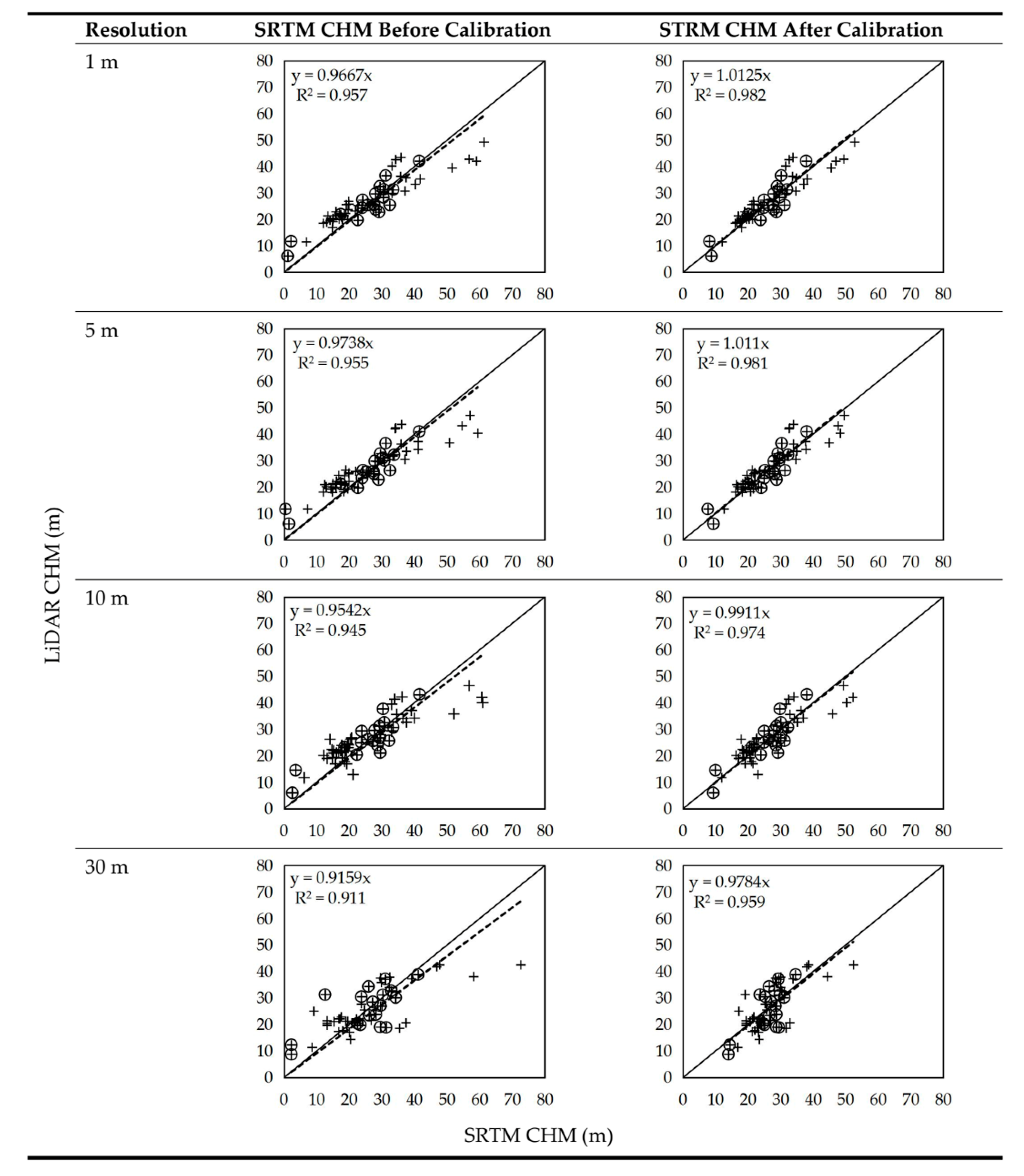
52]. This suggests that SRTM CHM can be calibrated using LiDAR CHM for AGB estimation if these CHMs are strongly correlated. In this study, the LiDAR CHM mean was strongly correlated with SRTM CHM except for 30 m resolution, thus allowing the calibration of SRTM CHM for spatial resolutions of 1, 5, and 10 m using the LiDAR CHM mean. While we found a high goodness-of-fit for the calibration models of the CHMs (R2 = 0.740–0.843) in the tropical montane forest, past studies indicate that the regression fit might depend on forest type. Notable regression fits were reported for the CHMs in mangrove and boreal pine forests [27,53] but not for the CHMs in boreal hardwood forests [53]. In this study, the calibrated SRTM CHMs showed an improved regression fit when plotted against the LiDAR CHMs (R2 ≥ 0.959) compared to the uncalibrated ones and became well distributed along the x = y line (Figure 3).
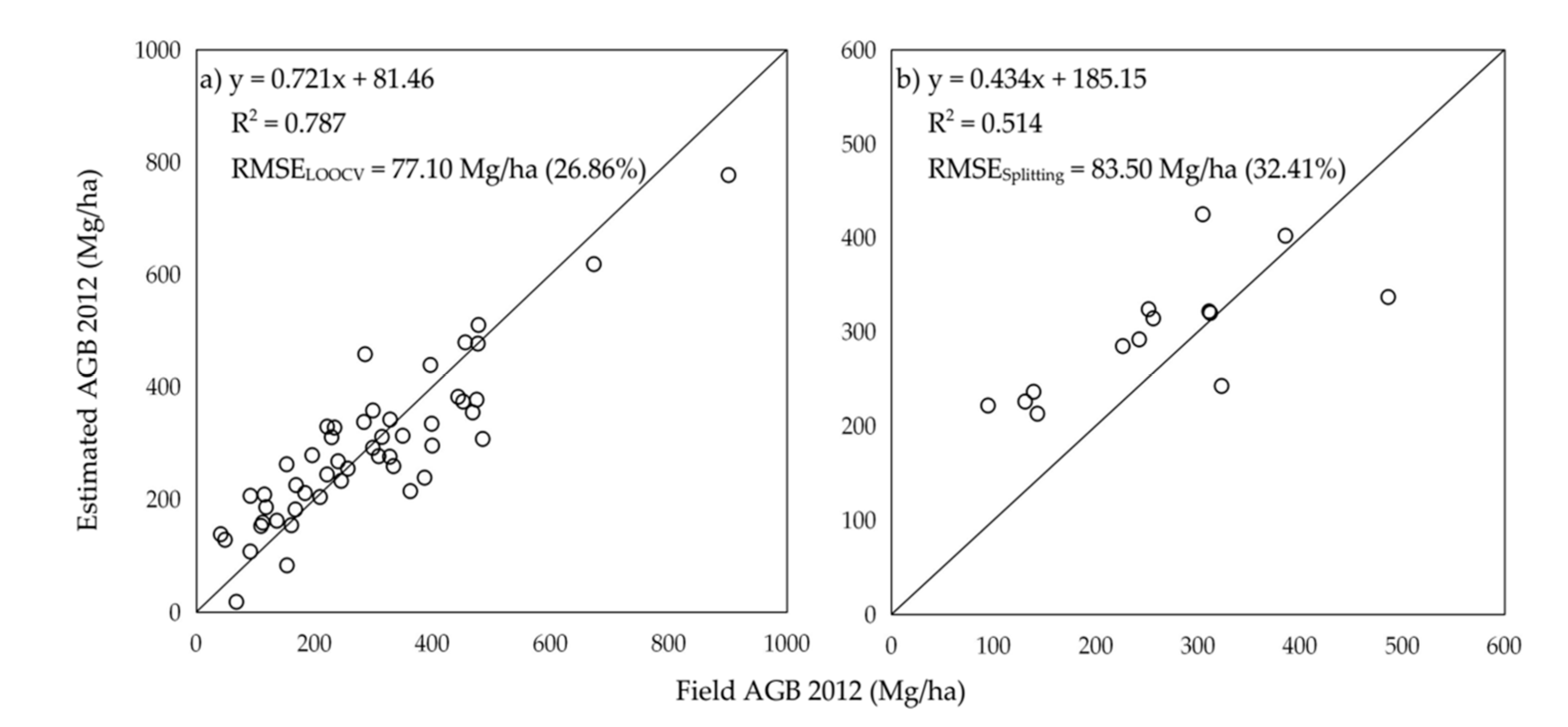
In the tropical montane forest, the LiDAR-CHM mean was examined as the estimator of field AGB for different spatial resolutions. The AGB estimation model using 1 m resolution LiDAR CHM had the best fit and explained the AGB variance better than other spatial resolutions in the regression analysis. The model EF decreased with decreasing the spatial resolution of the LiDAR CHM. When the LiDAR CHM resolution became coarser, the extracted information became more uncertain, thus leading to a decrease in spatial resolution. When the pixel size increased, the small forest canopy gaps could be overlooked, which could have led to an overestimation of the forest canopy height [54]. The best model using LiDAR CHM mean at 1 m resolution had a relatively low estimation error (RMSELOOCV = 77.10 Mg/ha, corresponding to about 26.86% of the average AGB). By randomly repeating the sample partitioning, we found that the relative RMSE of the independent validation ranged between 25.89% and 34.54%, with an average of 29.84%. Overall, these RMSE values were in a similar range to the RMSE of a multivariate AGB estimation model described by Ioki et al. (2014).
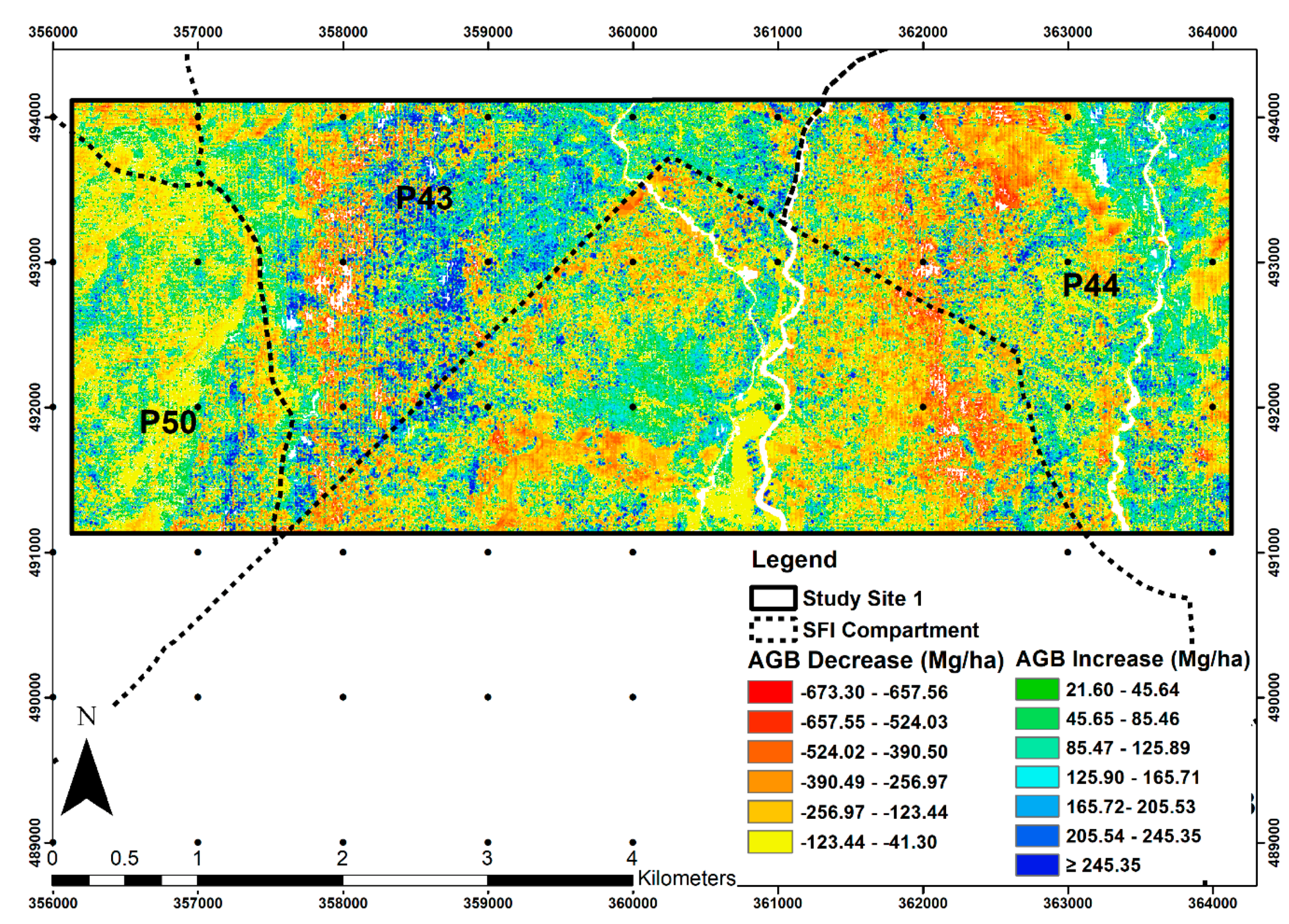
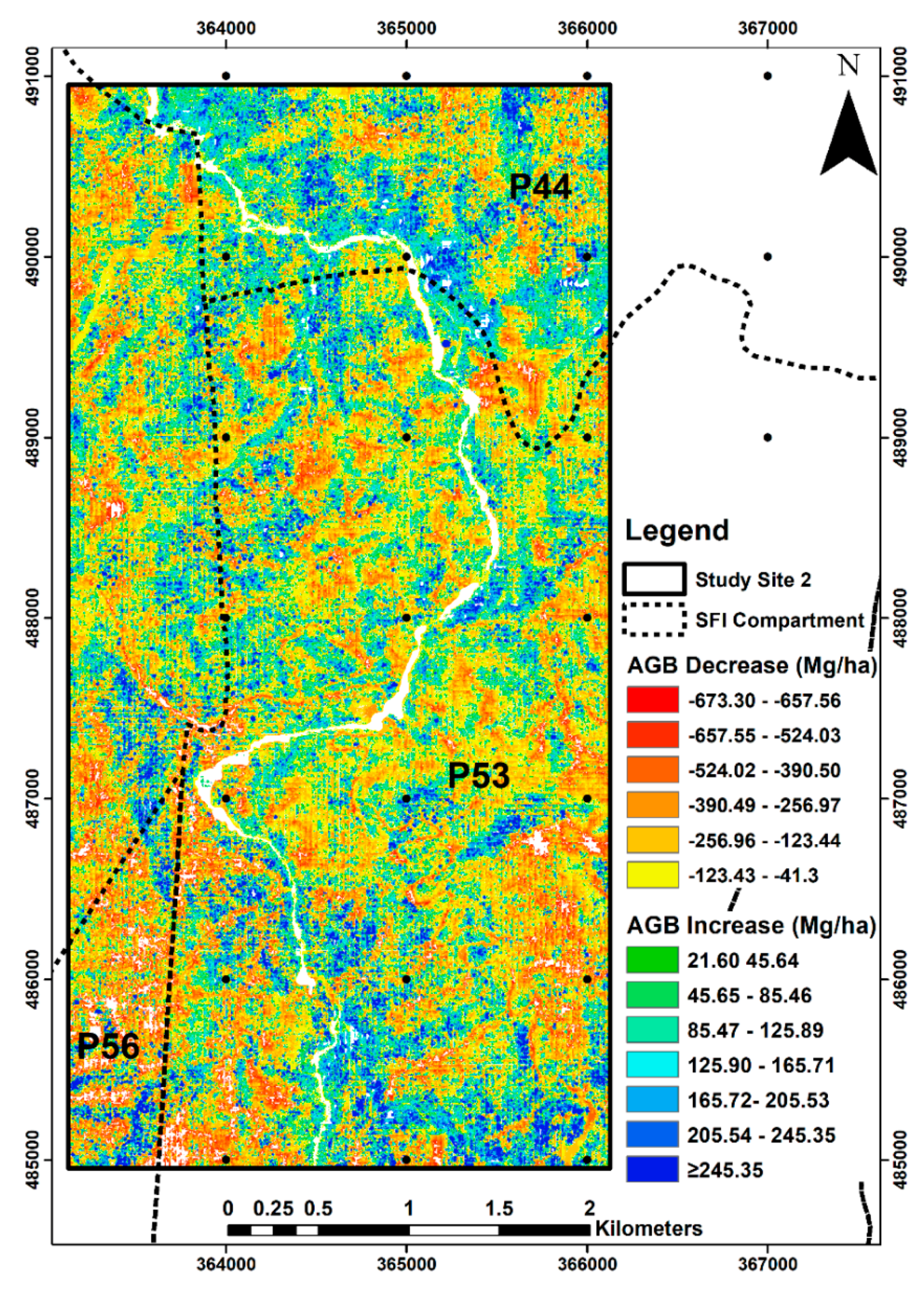
The time series AGB estimates allowed us to examine the pattern and driver of AGB changes in the study area. Most mountain communities in Sabah depend on slash-and-burn cultivation for their livelihoods, and this transforms the vegetation into a secondary forest landscape [
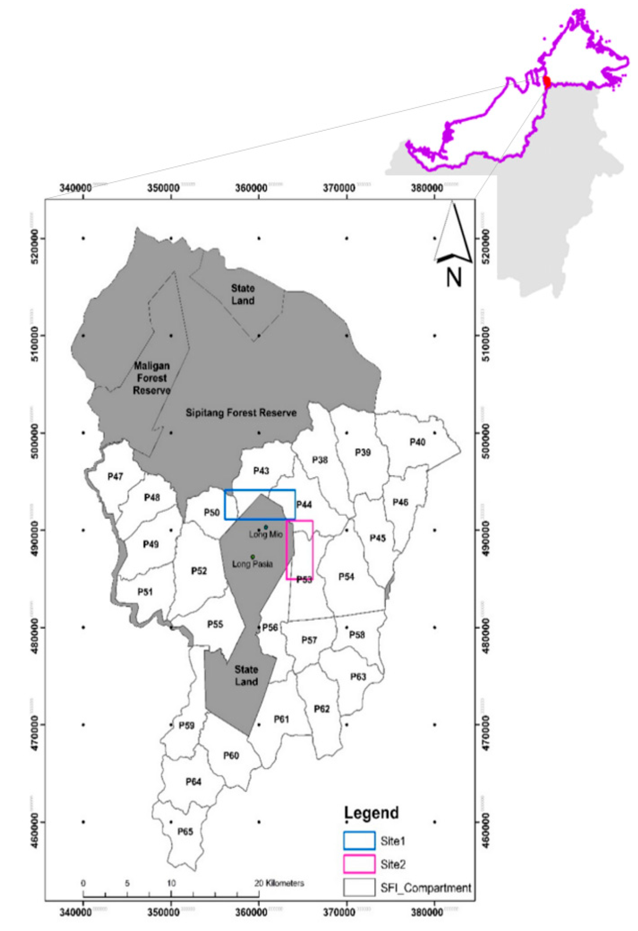
55]. Nevertheless, AGB removal by the local villagers is likely to be small-scale and limited to the immediately accessible areas. The main driver of AGB removal identified in this study was timber harvesting in the managed forests. The mean AGB decrease was 158.97 up to 673.30 Mg/ha, suggesting that timber extraction occurred in both logged-over and primary forests. The SFI confirmed that all compartments except compartment P50 at sites 1 and 2 were commercially logged. These logging activities started in 1997 and continued until the early 2000s when the state’s forestry policy changed from conventional logging to sustainable forest management [56].
Overall, there was a significant gain of AGB in the previously disturbed areas as a result of natural regeneration, especially in the managed forests. In a regenerating forest, small trees with DBH less than 10 cm can store up to 50% of the total AGB [57]. The mean AGB accumulation rate estimated in this study was 10.44 Mg/ha/yr over the 12 years. Our estimates match those reported elsewhere in the tropics. In a secondary tropical montane forest in southern Ecuador, the annual rate of AGB increase was estimated at 10 Mg/ha/yr [58]. In the montane forest of Mount Kinabalu, Sabah, the mean annual rates of aboveground net primary productivity range widely from 1.60 to 9.44 Mg C/ha/yr with a mean of 4.30 Mg C/ha/yr [59]. Figure 5 and 
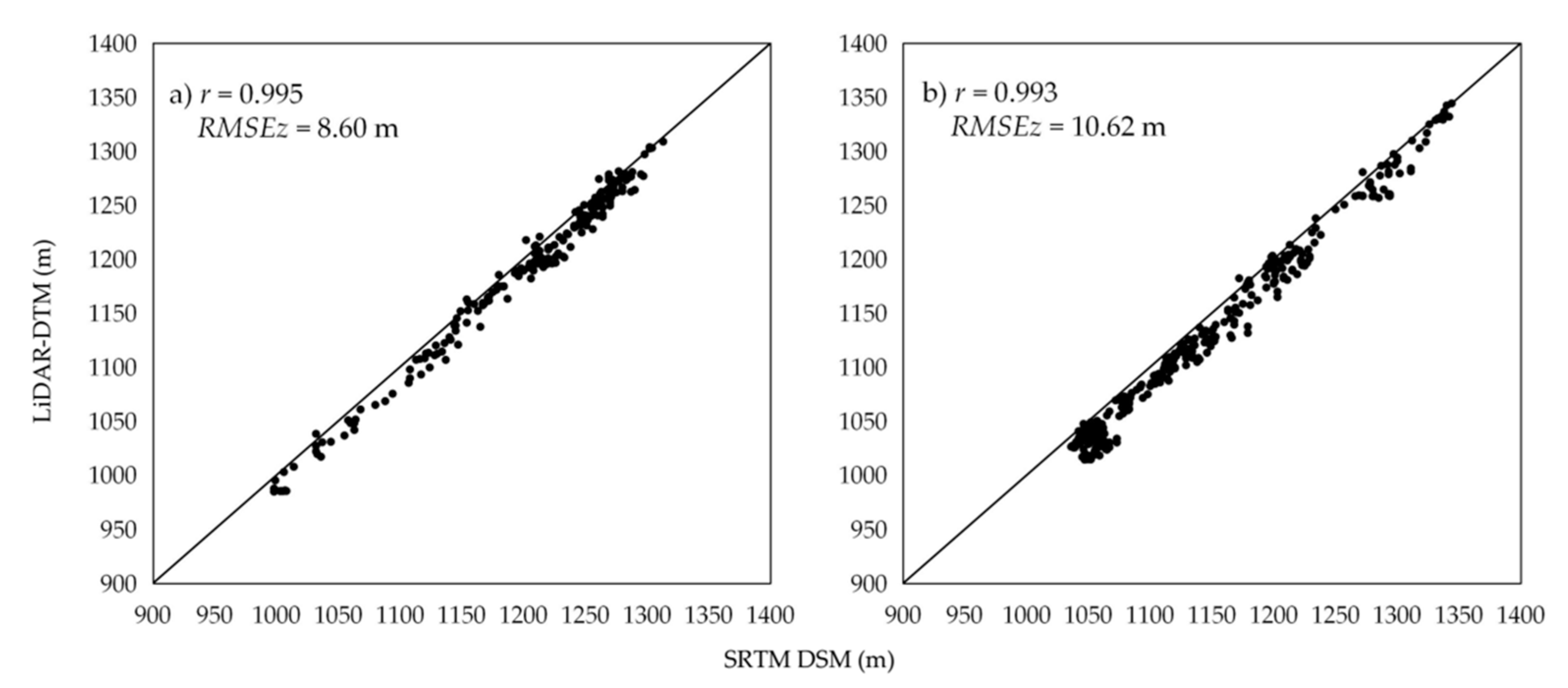
Figure 6 showed that some areas had AGB increases of more than three standard deviations (>20.4 Mg/ha/yr), which were likely to be overestimated. As LiDAR is currently the most accurate remote sensing method for estimating AGB, the overestimation was probably due to underestimation of the AGB 2000 values, especially in rugged terrain areas, because the accuracy of SRTM DSM of steep-sloped areas can be significantly affected by slope and aspect characteristics in relation to the incidence angle [60].

5. Conclusions

In the tropics, monitoring of AGB changes has been challenging due to a lack of historical AGB information. We examined the use of spaceborne (SRTM) and airborne (LiDAR) digital elevation data for estimating AGB changes in a tropical montane forest in northern Borneo between 2000 and 2012. Coupled with field data, an AGB estimation model was developed using the 1 m resolution LiDAR data. Not only was the AGB of 2012 estimated accurately, but the model can also be applied to estimate the historical AGB of 2000 by resampling and calibrating the SRTM DSM data. With the AGB estimates, it was possible to examine the AGB changes in two different land uses over the 12 years. As SRTM DSM data are freely available, this data can be used to estimate historical forest AGB as baseline information for monitoring forest changes in other tropical regions and to determine the main driver of AGB changes.

Author Contributions

M.-H.P. and S.T. framed the research questions and designed the study. M.-H.P., K.I. and W.V.C.W. designed the field data collection, which was carried out by D.J. and H.Y.L. Remotely sensed data processing and analysis were conducted by H.Y.L., D.J. and W.V.C.W. The first draft was prepared by H.Y.L. and M.-H.P. and K.I. reviewed and revised the manuscript. All authors have read and agreed to the published version of the manuscript.

Funding

This project was funded by the Ministry of Science, Technology and Innovation, Malaysia (Science Fund 04-01-10-SF0223) and Universiti Malaysia Sabah (GKP0005).

Acknowledgments

The authors would like to thank the generous assistance and cooperation of various parties involved in this study. We are grateful to Sabah Forestry Department for research permission and Sabah Forest Industries Sdn. Bhd. in particular for field supports. We are also thankful to the anonymous reviewers who provided valuable comments and suggestions for improvement of the manuscript.

Conflicts of Interest

The authors declare no conflict of interest.

References

  1. Le Quéré, C.; Raupach, M.R.; Canadell, J.G.; Marland, G.; Bopp, L.; Ciais, P.; Conway, T.J.; Doney, S.C.; Feely, R.A.; Foster, P.; et al. Trends in the sources and sinks of carbon dioxide. Nat. Geosci. 2009, 2, 831–836. [Google Scholar] [CrossRef]
  2. Eggleston, S.; Buendia, L.; Miwa, K.; Ngara, T.; Tanabe, K. (Eds.) 2006 IPCC Guidelines for National Greenhouse Gas Inventories; Institute for Global Environmental Strategies: Hayama, Japan, 2006; Volume 5. [Google Scholar]
  3. Langner, A.; Samejima, H.; Ong, R.C.; Titin, J.; Kitayama, K. Integration of carbon conservation into sustainable forest management using high resolution satellite imagery: A case study in Sabah, Malaysian Borneo. Int. J. Appl. Earth Obs. Geoinf. 2012, 18, 305–312. [Google Scholar] [CrossRef]
  4. Gaveau, D.L.A.; Salim, M.A.; Hergoualc’H, K.; Locatelli, B.; Sloan, S.; Wooster, M.; Marlier, M.E.; Molidena, E.; Yaen, H.; DeFries, R.; et al. Major atmospheric emissions from peat fires in Southeast Asia during non-drought years: Evidence from the 2013 Sumatran fires. Sci. Rep. 2014, 4, srep06112. [Google Scholar] [CrossRef] [PubMed] [Green Version]
  5. Broich, M.; Hansen, M.; Potapov, P.V.; Wimberly, M.C. Patterns of tree-cover loss along the Indonesia–Malaysia border on Borneo. Int. J. Remote Sens. 2013, 34, 5748–5760. [Google Scholar] [CrossRef]
  6. Maycock, C.R.; Nilus, R. Overview of the permanent vegetation plot network in Sabah. In Developing a Network of Long-Term Research Field Stations to Monitor Environmental Changes and Ecosystem Responses in Asian Forests; Kamata, N., Kuraji, K., Owari, T., Guan, B.T., Eds.; The University of Tokyo Forests Press: Tokyo, Japan, 2019; pp. 157–168. [Google Scholar]
  7. Stern, N. The Economics of Climate Change; Cambridge University Press: Cambridge, UK, 2007; p. 712. [Google Scholar]
  8. Gibbs, H.K.; Brown, S.; Niles, J.O.; Foley, J.A. Monitoring and estimating tropical forest carbon stocks: Making REDD a reality. Environ. Res. Lett. 2007, 2, 045023. [Google Scholar] [CrossRef]
  9. Koch, B. Status and future of laser scanning, synthetic aperture radar and hyperspectral remote sensing data for forest biomass assessment. ISPRS J. Photogramm. Remote Sens. 2010, 65, 581–590. [Google Scholar] [CrossRef]
  10. Dube, T.; Mutanga, O.; Elhadi, A.; Ismail, R.; Adam, E. Intra-and-Inter Species Biomass Prediction in a Plantation Forest: Testing the Utility of High Spatial Resolution Spaceborne Multispectral RapidEye Sensor and Advanced Machine Learning Algorithms. Sensors 2014, 14, 15348–15370. [Google Scholar] [CrossRef] [Green Version]
  11. Lu, D. The potential and challenge of remote sensing-based biomass estimation. Int. J. Remote Sens. 2006, 27, 1297–1328. [Google Scholar] [CrossRef]
  12. Mutanga, O.; Adam, E.; Cho, M.A. High density biomass estimation for wetland vegetation using WorldView-2 imagery and random forest regression algorithm. Int. J. Appl. Earth Obs. Geoinf. 2012, 18, 399–406. [Google Scholar] [CrossRef]
  13. Mutanga, O.; Skidmore, A.K. Narrow band vegetation indices overcome the saturation problem in biomass estimation. Int. J. Remote Sens. 2004, 25, 3999–4014. [Google Scholar] [CrossRef]
  14. Sarker, L.R.; Nichol, J.E. Improved forest biomass estimates using ALOS AVNIR-2 texture indices. Remote Sens. Environ. 2011, 115, 968–977. [Google Scholar] [CrossRef]
  15. Balzter, H.; Rowland, C.S.; Saich, P. Forest canopy height and carbon estimation at Monks Wood National Nature Reserve, UK, using dual-wavelength SAR interferometry. Remote Sens. Environ. 2007, 108, 224–239. [Google Scholar] [CrossRef]
  16. Englhart, S.; Keuck, V.; Siegert, F. Aboveground biomass retrieval in tropical forests—The potential of combined X- and L-band SAR data use. Remote Sens. Environ. 2011, 115, 1260–1271. [Google Scholar] [CrossRef]
  17. Mitchard, E.T.A.; Saatchi, S.S.; Woodhouse, I.H.; Nangendo, G.; Ribeiro, N.S.; Williams, M.; Ryan, C.M.; Lewis, S.L.; Feldpausch, T.R.; Meir, P. Using satellite radar backscatter to predict above-ground woody biomass: A consistent relationship across four different African landscapes. Geophys. Res. Lett. 2009, 36, 36. [Google Scholar] [CrossRef]
  18. Mitchard, E.T.A.; Saatchi, S.; Lewis, S.L.; Feldpausch, T.R.; Woodhouse, I.; Sonke, B.; Rowland, C.S.; Meir, P. Measuring biomass changes due to woody encroachment and deforestation/degradation in a forest–savanna boundary region of central Africa using multi-temporal L-band radar backscatter. Remote Sens. Environ. 2011, 115, 2861–2873. [Google Scholar] [CrossRef] [Green Version]
  19. Neeff, T.; Dutra, L.V.; dos Santos, J.R.; Freitas, C.D.C.; Araujo, L.S. Tropical forest measurement by interferometric height modeling and P-band radar backscatter. For. Sci. 2005, 51, 585–594. [Google Scholar] [CrossRef]
  20. Farr, T.G.; Rosen, P.A.; Caro, E.; Crippen, R.; Duren, R.; Hensley, S.; Kobrick, M.; Paller, M.; Rodriguez, E.; Roth, L.; et al. The Shuttle Radar Topography Mission. Rev. Geophys. 2007, 45, 45. [Google Scholar] [CrossRef] [Green Version]
  21. Bhang, K.J.; Schwartz, F.W.; Braun, A. Verification of the Vertical Error in C-Band SRTM DEM Using ICESat and Landsat-7, Otter Tail County, MN. IEEE Trans. Geosci. Remote Sens. 2006, 45, 36–44. [Google Scholar] [CrossRef]
  22. Hofton, M.; Dubayah, R.; Blair, J.B.; Rabine, D. Validation of SRTM Elevations over Vegetated and Non-vegetated Terrain Using Medium Footprint Lidar. Photogramm. Eng. Remote Sens. 2006, 72, 279–285. [Google Scholar] [CrossRef] [Green Version]
  23. Su, Y.; Guo, Q. A practical method for SRTM DEM correction over vegetated mountain areas. ISPRS J. Photogramm. Remote Sens. 2014, 87, 216–228. [Google Scholar] [CrossRef]
  24. Fatoyinbo, T.; Simard, M. Height and biomass of mangroves in Africa from ICESat/GLAS and SRTM. Int. J. Remote Sens. 2012, 34, 668–681. [Google Scholar] [CrossRef]
  25. Goïta, K.; Mouloungou, J.; Bénié, G.B. Estimation of aboveground biomass and carbon in a tropical rain forest in Gabon using remote sensing and GPS data. Geocarto Int. 2017, 34, 243–259. [Google Scholar] [CrossRef]
  26. Kellndorfer, J.; Walker, W.; Pierce, L.; Dobson, C.; Fites, J.A.; Hunsaker, C.T.; Vona, J.; Clutter, M. Vegetation height estimation from Shuttle Radar Topography Mission and National Elevation Datasets. Remote Sens. Environ. 2004, 93, 339–358. [Google Scholar] [CrossRef]
  27. Lagomasino, D.; Fatoyinbo, T.; Lee, S.-K.; Feliciano, E.; Trettin, C.C.; Simard, M. A Comparison of Mangrove Canopy Height Using Multiple Independent Measurements from Land, Air, and Space. Remote Sens. 2016, 8, 327. [Google Scholar] [CrossRef] [Green Version]
  28. Dubayah, R.O.; Drake, J.B. Lidar remote sensing for forestry. J. For. 2000, 98, 44–46. [Google Scholar] [CrossRef]
  29. Asner, G.P.; Mascaro, J.; Muller-Landau, H.C.; Vieilledent, G.; Vaudry, R.; Rasamoelina, M.; Hall, J.S.; Van Breugel, M. A universal airborne LiDAR approach for tropical forest carbon mapping. Oecologia 2011, 168, 1147–1160. [Google Scholar] [CrossRef]
  30. Hayashi, M.; Saigusa, N.; Yamagata, Y.; Hirano, T. Regional forest biomass estimation using ICESat/GLAS spaceborne LiDAR over Borneo. Carbon Manag. 2015, 6, 19–33. [Google Scholar] [CrossRef]
  31. Keller, M.; Lefsky, M.A.; Pang, Y.; De Camargo, P.B.; Hunter, M.O. Revised method for forest canopy height estimation from Geoscience Laser Altimeter System waveforms. J. Appl. Remote Sens. 2007, 1, 013537. [Google Scholar] [CrossRef]
  32. Sun, G.; Ranson, K.J.; Guo, Z.; Zhang, Z.; Montesano, P.; Kimes, D. Forest biomass mapping from lidar and radar synergies. Remote Sens. Environ. 2011, 115, 2906–2916. [Google Scholar] [CrossRef] [Green Version]
  33. Zhao, K.; Popescu, S. Hierarchical watershed segmentation of canopy height model for multi—Scale forest inventory. Proc. ISPRS Work. Group Laser Scanning 2007, XXXVI, 436–442. [Google Scholar]
  34. Phua, M.-H.; Hue, S.W.; Ioki, K.; Hashim, M.; Bidin, K.; Musta, B.; Suleiman, M.; Yap, S.W.; Maycock, C. Estimating Logged-Over Lowland Rainforest Aboveground Biomass in Sabah, Malaysia Using Airborne LiDAR Data. Terr. Atmos. Ocean. Sci. 2016, 27, 481. [Google Scholar] [CrossRef] [Green Version]
  35. Coomes, D.A.; Dalponte, M.; Jucker, T.; Asner, G.P.; Banin, L.; Burslem, D.F.; Lewis, S.L.; Nilus, R.; Phillips, O.L.; Phua, M.-H.; et al. Area-based vs tree-centric approaches to mapping forest carbon in Southeast Asian forests from airborne laser scanning data. Remote Sens. Environ. 2017, 194, 77–88. [Google Scholar] [CrossRef] [Green Version]
  36. Phua, M.-H.; Johari, S.A.; Wong, O.C.; Ioki, K.; Mahali, M.; Nilus, R.; Coomes, D.A.; Maycock, C.R.; Hashim, M. Synergistic use of Landsat 8 OLI image and airborne LiDAR data for above-ground biomass estimation in tropical lowland rainforests. For. Ecol. Manag. 2017, 406, 163–171. [Google Scholar] [CrossRef]
  37. Skowronski, N.S.; Clark, K.L.; Gallagher, M.; Birdsey, R.A.; Hom, J.L. Airborne laser scanner-assisted estimation of aboveground biomass change in a temperate oak–pine forest. Remote Sens. Environ. 2014, 151, 166–174. [Google Scholar] [CrossRef]
  38. Takagi, K.; Yone, Y.; Takahashi, H.; Sakai, R.; Hojyo, H.; Kamiura, T.; Nomura, M.; Liang, N.; Fukazawa, T.; Miya, H.; et al. Forest biomass and volume estimation using airborne LiDAR in a cool-temperate forest of northern Hokkaido, Japan. Ecol. Inform. 2015, 26, 54–60. [Google Scholar] [CrossRef]
  39. McRoberts, R.E.; Næsset, E.; Gobakken, T.; Bollandsås, O.M. Indirect and direct estimation of forest biomass change using forest inventory and airborne laser scanning data. Remote Sens. Environ. 2015, 164, 36–42. [Google Scholar] [CrossRef]
  40. Bollandsås, O.M.; Gregoire, T.G.; Næsset, E.; Øyen, B.-H. Detection of biomass change in a Norwegian mountain forest area using small footprint airborne laser scanner data. J. Ital. Stat. Soc. 2012, 22, 113–129. [Google Scholar] [CrossRef]
  41. Hudak, A.T.; Strand, E.K.; Vierling, L.A.; Byrne, J.C.; Eitel, J.U.; Martinuzzi, S.; Falkowski, M.J. Quantifying aboveground forest carbon pools and fluxes from repeat LiDAR surveys. Remote Sens. Environ. 2012, 123, 25–40. [Google Scholar] [CrossRef] [Green Version]
  42. De Moura, Y.M.; Balzter, H.; Galvão, L.S.; Dalagnol, R.; Espírito-Santo, F.; Santos, E.G.; García, M.; Bispo, P.D.C.; De Oliveira, R.C.; Shimabukuro, Y.E. Carbon Dynamics in a Human-Modified Tropical Forest: A Case Study Using Multi-Temporal LiDAR Data. Remote Sens. 2020, 12, 430. [Google Scholar] [CrossRef] [Green Version]
  43. Réjou-Méchain, M.; Tymen, B.; Blanc, L.; Fauset, S.; Feldpausch, T.R.; Monteagudo, A.; Phillips, O.L.; Richard, H.; Chave, J. Using repeated small-footprint LiDAR acquisitions to infer spatial and temporal variations of a high-biomass Neotropical forest. Remote Sens. Environ. 2015, 169, 93–101. [Google Scholar] [CrossRef]
  44. Vaz, J. An Analysis of International Law, National Legislation, Judgements, and Institutions as they Interrelate with Territories and Areas Conserved by Indigenous Peoples and Local Communities: No. 15 Malaysia; Natural Justice in Bangalore and Kalpavriksh: Delhi, India, 2012. [Google Scholar]
  45. Wong, W.V.C.; Tsuyuki, S.; Ioki, K.; Phua, M.H. Accuracy assessment of global topographic data (SRTM & ASTER GDEM) in comparison with lidar for tropical montane forest. In Proceedings of the 35th Asian Conference on Remote Sensing 2014, ACRS 2014: Sensing for Reintegration of Societies, Nay Pyi Taw, Myanmar, 27–31 October 2014; pp. 27–31. [Google Scholar]
  46. Simard, M.; Zhang, K.; Rivera-Monroy, V.H.; Ross, M.S.; Ruiz, P.L.; Castañeda-Moya, E.; Twilley, R.R.; Rodriguez, E. Mapping Height and Biomass of Mangrove Forests in Everglades National Park with SRTM Elevation Data. Photogramm. Eng. Remote Sens. 2006, 72, 299–311. [Google Scholar] [CrossRef]
  47. Chave, J.; Réjou-Méchain, M.; Búrquez, A.; Chidumayo, E.; Colgan, M.S.; Delitti, W.B.C.; Duque, A.; Eid, T.; Fearnside, P.M.; Goodman, R.C.; et al. Improved allometric models to estimate the aboveground biomass of tropical trees. Glob. Chang. Biol. 2014, 20, 3177–3190. [Google Scholar] [CrossRef]
  48. Giancristofaro, R.A.; Salmaso, L. Model Performance Analysis and Model Validation in Logistic Regression. Statistica 2007, 63, 375–396. [Google Scholar] [CrossRef]
  49. Vanclay, J.K.; Skovsgaard, J. Evaluating forest growth models. Ecol. Model. 1997, 98, 1–12. [Google Scholar] [CrossRef] [Green Version]
  50. Baskerville, G.L. Use of Logarithmic Regression in the Estimation of Plant Biomass. Can. J. For. Res. 1972, 2, 49–53. [Google Scholar] [CrossRef]
  51. Clark, M.L.; Roberts, D.A.; Ewel, J.J.; Clark, D.B. Estimation of tropical rain forest aboveground biomass with small-footprint lidar and hyperspectral sensors. Remote Sens. Environ. 2011, 115, 2931–2942. [Google Scholar] [CrossRef]
  52. Jochem, A.; Hollaus, M.; Rutzinger, M.; Höfle, B.; Schadauer, K.; Maier, B. Estimation of aboveground biomass using airborne LiDAR data. In Proceedings of the 10th International Conference on LiDAR Applications for Assessing Forest Ecosystems (Silvilaser 2010), Freiburg, Germany, 14–17 September 2010; pp. 14–17. [Google Scholar]
  53. Sexton, J.O.; Bax, T.; Siqueira, P.; Swenson, J.J.; Hensley, S. A comparison of lidar, radar, and field measurements of canopy height in pine and hardwood forests of southeastern North America. For. Ecol. Manag. 2009, 257, 1136–1147. [Google Scholar] [CrossRef]
  54. Mascaró, J.; Asner, G.P.; Muller-Landau, H.C.; Van Breugel, M.; Hall, J.; Dahlin, K. Controls over aboveground forest carbon density on Barro Colorado Island, Panama. Biogeosciences 2011, 8, 1615–1629. [Google Scholar] [CrossRef] [Green Version]
  55. Ioki, K.; Tsuyuki, S.; Hirata, Y.; Phua, M.-H.; Wong, W.V.C.; Ling, Z.-Y.; Saito, H.; Takao, G. Estimating above-ground biomass of tropical rainforest of different degradation levels in Northern Borneo using airborne LiDAR. For. Ecol. Manag. 2014, 328, 335–341. [Google Scholar] [CrossRef]
  56. Sabah Forestry Department. Identification of Potential Protected Areas: Ulu Padas Sabah Biodiversity Conservation Project Final Report; Sabah Forestry Department: Sandakan, Malaysia, 1998.
  57. Markesteijn, L.; Poorter, L. Seedling root morphology and biomass allocation of 62 tropical tree species in relation to drought- and shade-tolerance. J. Ecol. 2009, 97, 311–325. [Google Scholar] [CrossRef]
  58. Spracklen, D.V.; Righelato, R. Carbon storage and sequestration of re-growing montane forests in southern Ecuador. For. Ecol. Manag. 2016, 364, 139–144. [Google Scholar] [CrossRef] [Green Version]
  59. Kitayama, K.; Aiba, S.-I. Ecosystem structure and productivity of tropical rain forests along altitudinal gradients with contrasting soil phosphorus pools on Mount Kinabalu, Borneo. J. Ecol. 2002, 90, 37–51. [Google Scholar] [CrossRef]
  60. Gorokhovich, Y.; Voustianiouk, A. Accuracy assessment of the processed SRTM-based elevation data by CGIAR using field data from USA and Thailand and its relation to the terrain characteristics. Remote Sens. Environ. 2006, 104, 409–415. [Google Scholar] [CrossRef]
Figure 1. Map of the study area. Ulu Padas, Sabah, Malaysia.
Remotesensing 12 03677 g001
Figure 2. Scatterplot between Shuttle Radar Topographic Mission Digital Elevation Model (SRTM) digital surface model (DSM) and Light Detection and Ranging (LiDAR)-DTM for bare surfaces in (a) site 1 and (b) site 2.
Remotesensing 12 03677 g002
Figure 3. The relationship between LiDAR CHM and SRTM CHM before and after calibration in different spatial resolutions. The calibrated SRTM CHM values of 18 field plots of old-growth forest that were used for the calibration (circle) and additional 40 old-growth forest locations (cross) showed an improved regression fit to the LiDAR CHM values especially for 1 and 5 m resolutions (R2 ≥ 0.98).
Remotesensing 12 03677 g003
Figure 4. Scatterplot between field AGB and LiDAR estimated AGB using the best model for (a) Modelling plots. (b) Independent validation plots.
Remotesensing 12 03677 g004
Figure 5. AGB changes between 2000 and 2012 in site 1. The increase was mostly within three standard deviations, occurring at previously logged areas especially in compartment P43.
Remotesensing 12 03677 g005
Figure 6. AGB changes between 2000 and 2012 in site 2.
Remotesensing 12 03677 g006
Table 1. Correlation and differences between SRTM DSM and LiDAR DTM for bare grounds.
MeasuresStudy Site 1Study Site 2
r0.995 **0.993 **
RMSE8.60 m10.62 m
biasz6.66 m8.93 m
rbiasz0.56%0.79%
** Correlation is significant at the 0.01 level (2-tailed).
Table 2. Pearson’s correlations between the field measured mean height and the derived canopy height model (CHM) mean from airborne LiDAR and SRTM data (n = 18).
Resolution Mean Height (m)LiDAR CHM (m)SRTM CHM (m)
1 mMean height (m)1
LiDAR CHM (m)0.875 **1
SRTM CHM (m)0.846 **0.906 **1
5 mMean height (m)1
LiDAR CHM (m)0.874 **1
SRTM CHM (m)0.844 **0.918 **1
10 mMean height (m)1
LiDAR CHM (m)0.861 **1
SRTM CHM (m)0.838 **0.860 **1
30 mMean height (m)1
LiDAR CHM (m)0.701 **1
SRTM CHM (m)0.839 **0.683 **1
** Correlation is significant at the 0.01 level (2-tailed).
Table 3. SRTM CHM calibration models.
(Constant)Coefficient
ResolutionModelR2Std. Error of the EstimatetSig.tSig.
1 mSRTM CHMCal = 0.747(SRTM CHM) + 6.93670.8213.6072.9170.0018.5640.000
5 mSRTM CHMCal = 0.7418(SRTM CHM) + 7.23750.8433.3663.3280.0049.2840.000
10 mSRTM CHMCal = 0.7394(SRTM CHM) + 7.35530.7404.3122.4720.0256.7550.009
30 mSRTM CHMCal = 0.5557(SRTM CHM) + 12.0320.4676.2362.9940.0093.7450.002
SRTM CHMCal: Calibrated SRTM CHM.
Table 4. Summary of field measurements in the study area.
SiteDBH, (cm)Tree Height, (m)Wood Density, (g/cm3)AGB, (Mg/ha)
MeanMax *SD **MeanMax *SD **MeanMax *SD **MeanMax *SD **
119.33109.904.6817.6665.902.320.611.050.04292.15901.29164.45
218.98122.103.6117.0329.354.530.581.060.04243.01468.04118.01
* maximum; ** standard deviation.
Table 5. Aboveground biomass (AGB) estimation models using LiDAR CHM of different spatial resolutions.
ResolutionModelEFRMSEModel (Mg/ha)Relative RMSEModel (%)
1 mLn(AGB) = 1.721[Ln(CHMmean 1 m)] + 0.17190.79874.1025.81
5 mLn(AGB) = 1.6813[Ln(CHMmean 5 m)] + 0.290.76879.2827.62
10 mLn(AGB) = 1.719[Ln(CHMmean 10 m)] + 0.1670.79774.0425.79
30 mLn(AGB) = 0.501[Ln(CHMmean 30 m)] + 3.9610.288139.1048.45
Table 6. Summary of AGB changes in the study area.
AGB Increase (Mg/ha)
MinimumMeanMaximumSD 1
Overall21.60125.29901.3039.82
Managed forests82.50122.57901.3034.67
Village areas21.6099.70137.6533.54
AGB Decrease (Mg/ha)
Overall−41.30−390.50−673.30133.53
Managed forests−95.45−158.97−673.3058.42
Village areas−41.30−154.90−274.108.87
1 SD is standard deviation.
Publisher’s Note: MDPI stays neutral with regard to jurisdictional claims in published maps and institutional affiliations.

