Next Article in Journal
Combining Evolutionary Algorithms and Machine Learning Models in Landslide Susceptibility Assessments
Next Article in Special Issue
A Comprehensive Forest Biomass Dataset for the USA Allows Customized Validation of Remotely Sensed Biomass Estimates
Previous Article in Journal
Perspectives on the Structural Health Monitoring of Bridges by Synthetic Aperture Radar
Previous Article in Special Issue
Aboveground Biomass Changes in Tropical Montane Forest of Northern Borneo Estimated Using Spaceborne and Airborne Digital Elevation Data
 
 
Correction published on 10 October 2022, see Remote Sens. 2022, 14(19), 5044.
Article

High-Precision Stand Age Data Facilitate the Estimation of Rubber Plantation Biomass: A Case Study of Hainan Island, China

1
Danzhou Investigation & Experiment Station of Tropical Cops, State Key Laboratory Incubation Base for Cultivation & Physiology of Tropical Crops, Rubber Research Institute (RRI), Chinese Academy of Tropical Agricultural Sciences (CATAS), Haikou 571101, China
2
College of Forestry, Nanjing Forestry University, Nanjing 210037, China
3
Ministry of Education Key Laboratory for Biodiversity Science and Ecological Engineering, Institute of Biodiversity Science, Fudan University, No. 2005, Songhu Road, Shanghai 200438, China
4
College of Big Data and Intelligence Engineering, Southwest Forestry University, Kunming 650224, China
5
Institute of Scientific and Technical Information, Chinese Academy of Tropical Agricultural Sciences (CATAS), Haikou 571101, China
6
Department of Microbiology and Plant Biology, Center for Spatial Analysis, University of Oklahoma, Norman, OK 73019, USA
*
Author to whom correspondence should be addressed.
Remote Sens. 2020, 12(23), 3853; https://doi.org/10.3390/rs12233853
Submission received: 30 September 2020 / Revised: 14 November 2020 / Accepted: 18 November 2020 / Published: 24 November 2020 / Corrected: 10 October 2022
(This article belongs to the Special Issue Forest Biomass and Carbon Observation with Remote Sensing)

Abstract

:
Rubber (Hevea brasiliensis Muell.) plantations constitute one of the most important agro-ecosystems in the tropical region of China and Southeast Asia, playing an important role in the carbon budget there. Accurately obtaining their biomass over a large area is challenging because of difficulties in acquiring the Diameter at Breast Height (DBH) through remote sensing and the problem of biomass saturation. The stand age, which is closely related to the forest biomass, was proposed for biomass estimation in this study. A stand age map at an annual scale for Hainan Island, which is the second largest natural rubber production base in China, was generated using all Landsat and Sentinel-2 (LS2) data (1987–2017). Scatter plots and the correlation coefficient method were used to explore the relationship (e.g., biomass saturation) between rubber biomass and different LS2-based variables. Subsequently, a regression model fitted with the stand age (R2 = 0.96) and a Random Forest (RF) model parameterizing with LS2-based variables and/or the stand age were respectively employed to estimate rubber biomass for Hainan Island. The results show that rubber biomass was saturated around 65 Mg/ha with all LS2-based variables. The regression model estimated biomass accurately (R2 = 0.79 and Root Mean Square Error (RMSE) = 14.00 Mg/ha) and eliminated the saturation problem significantly. In addition to LS2-based variables, adding a stand age parameter to the RF models was found to significantly improve the prediction accuracy (R2 = 0.82–0.96 and RMSE = 4.08–10.59 Mg/ha, modeling using samples of different biomass sizes). However, all RF models overestimated the biomass of young plantations and underestimated the biomass of old plantations. A hybrid model integrating the optimal results of RF and regression models reduced estimation bias and generated the best performance (R2 = 0.83 and RMSE = 12.48 Mg/ha). The total rubber biomass of Hainan Island in 2017 was about 5.40 × 10⁷ Mg. The northward and westward expansions after 2000 had great impact on the biomass distribution, leading to a higher biomass density for the inland coastal strip from south to northeast and a lower biomass density in the northern and western regions.

Graphical Abstract

1. Introduction

The rubber tree (Hevea brasiliensis Muell.), which is widely planted in tropical regions such as Southeast Asia and the tropical region of China, is of great importance in producing natural rubber and in providing timber when the rubber latex harvest is finished [1,2]. The establishment of new rubber plantations—usually converted from old rubber plantations, tropical forest, and cropland [3]—and timber harvesting in old rubber plantations will greatly alter the carbon budget [4]. Therefore, accurately estimating biomass, which is an important indicator of the carbon storage capacity and the potential carbon pool size of a forest ecosystem [5,6], is a widespread concern of ecologists, plantation managers, and policy makers related to the rubber industry.
The biomass of rubber plantations at a plot level is usually estimated by allometric equation (AE) models, linked with field measurements of the Diameter at Breast Height (DBH) and Height (H), or a combination of other factors, such as the stand age and wood density [7,8,9,10,11]. In China, four rubber biomass allometric models have been developed thus far [8,10,12,13]. All these models use DBH or the combination of DBH and H as independent variables, yielding R2 values greater than 0.97. Three of these models were developed in Xishuangbanna prefecture, Yunnan Province [8,10,12], and one was developed in Leizhou Peninsula (close to Hainan island), Guangdong Province [13]. Jia et al.’s [12] model only considers the aboveground biomass but covers biomass variation at low (550–600 m), medium (750–800 m), and high (950–1050 m) elevations above the mean sea level (AMSL), while the other three models consider the belowground biomass [8,10,13]. These AE models are very valuable because the purpose of planting rubber trees is to harvest latex for a long period of time (usually 25–30 years) instead of wood. The cost of felling mature rubber trees in a large area to establish AE models is very high.
There are several ways to extend biomass at the tree/plot level to a landscape/regional scale. One of the commonly used methods is to convert tree volume data from forest inventories into biomass using biomass conversion and expansion factors (BCEFs) [14,15,16]. A generalized curve of BCEFs for different species or species groups by stand age and site index has been developed in most countries, such as Poland and China, which signed up for the United Nations Framework Convention on Climate Change (UNFCCC) and its supplementary Kyoto Protocol [14,17]. Another approach is to multiply the average or time-averaged biomass obtained at a plot scale by the area in a specific region [11,18]. For example, Petsri et al. [9] calculated the biomass per hectare through a meta-analysis of DBH and H against stand age and then estimated the national rubber biomass in Thailand with annual statistics for area data and a fixed rotation length of 25 years. The accuracy obtained in this way was much better than the result obtained from multiplying the average/time averaged biomass by the total area. However, large uncertainties may exist because the actual age structure is unknown and the rotation length is not fixed at 25 years. In addition, the use of remote sensing to estimate forest biomass over a large area is becoming increasingly popular. Many studies has been conducted to estimate different forest (e.g., broadleaf and coniferous) biomass through optical satellite imagery [19,20,21], the Synthetic Aperture Radar (SAR) [6,22,23], Light Detection and Ranging (LiDAR) [24,25], or their combination [23,26,27,28,29]. More recently, the European Space Agency planned to launch a fully polarimetric P-band SAR satellite—BIOMASS—for which the main tasks are mapping the global aboveground biomass, forest height, and severe forest disturbances [30]. Generally, LiDAR is the top-ranked approach for forest biomass estimation as it can remove data saturation, followed by longer wavelength radar and optical remote sensing [31]. However, the data availability is the opposite; LiDAR data are the scarcest due to limited satellites carrying LiDAR instruments, and optical remote sensing data are the most abundant.
Many studies have used remote sensing to estimate the biomass of rubber plantations. The relationship between rubber biomass, spectral bands, and vegetation indices derived from Landsat Thematic Mapper (TM) was explored in Xishuangbanna Prefecture, Yunnan Province, China, and different biomass models using stepwise regression [32,33] and Random Forest (RF) [34] were developed (R2 = 0.43–0.67 and Root Mean Square Error (RMSE) = 30.27–46.05 Mg/ha). The total rubber biomass in Xishuangbanna was about 1.97 × 10⁷ Mg, and the average biomass was 75.90 Mg/ha [32]. Yasen and Koedsin found that an artificial neural network based on WorldView-2 multispectral imagery could estimate biomass more accurately than stepwise multiple linear regression in Phuket Province, Thailand [2]. Charoenjit et al. [35] first estimated tree girth—using spectral bands, textural parameters, and vegetation indices from Thaichote multispectral imagery by a linear multiple regression model—and then used it with an AE model to estimate the rubber biomass in eastern Thailand. Avtar et al. [36] found that the Horizontal transmitting with Vertical receiving (HV) band of the Phase-Array L-band Synthetic Aperture Radar (PALSAR) positively correlated with the biomass of rubber plantations. The correlation was higher than for the Horizontal transmitting with Horizontal receiving (HH) band, but it began to saturate when the biomass was about 50 Mg/ha. Trisaongko and Paull estimated the biomass of rubber plantations with a very high accuracy (R2 = 0.98 and RMSE = 1.88 Mg/ha), indicating that the acquisition time of PALSAR-2 and the choice of AE model significantly affect the accuracy [37]. By summarizing this literature, two main approaches for estimating the biomass of rubber plantations on a large scale can be obtained: (1) establishing direct relationships between biomass and spectral/SAR bands, vegetation indices, and textural parameters and (2) obtaining proxy factors such as DBH from remote sensing data and then using them as the parameters of AE models. In fact, all these approaches use canopy features from optical or SAR satellite imagery to estimate biomass. As the relationship between rubber biomass and canopy features gradually weakens with an increase in the stand age [38], the estimated biomass of middle-aged and old rubber plantations often exhibits large deviations.
There is also a close relationship between rubber biomass and stand age [39]. Good models (R2 = 0.97–0.99) of the biomass/carbon stock of rubber plantations and stand age have been developed in Xishuangbanna, Yunnan Province [8,40,41] and in Thailand [9]. Compared to DBH, the rubber stand age is easier to acquire accurately from time-series satellite imagery. Thanks to the free access of Landsat data policy [42], the establishment year (same as the stand age) of rubber plantations can be accurately traced back to the end of the 1980s at an annual resolution and RMSE of about 2 years [3,43], demonstrating great potential for biomass estimation. In addition to the stand age, the rubber biomass is also closely related to the geographical environment in which it grows, such as light conditions, soil moisture, and fertility. Differences in the growth condition of rubber plantations may affect the intensity of the spectral reflectance that can be used to estimate the biomass [35]. Therefore, we assume that combining the stand age and spectral characteristics can more accurately estimate the biomass of rubber plantations. The objectives of this study are (1) to explore the relationship between rubber biomass and stand age and LS2-based variables (e.g., spectral bands and vegetation indices); (2) to develop biomass models using stand age and LS2-based variables; and (3) to generate a biomass map of rubber plantations in Hainan Island, China and to investigate its spatial distribution pattern.

2. Materials and Methods
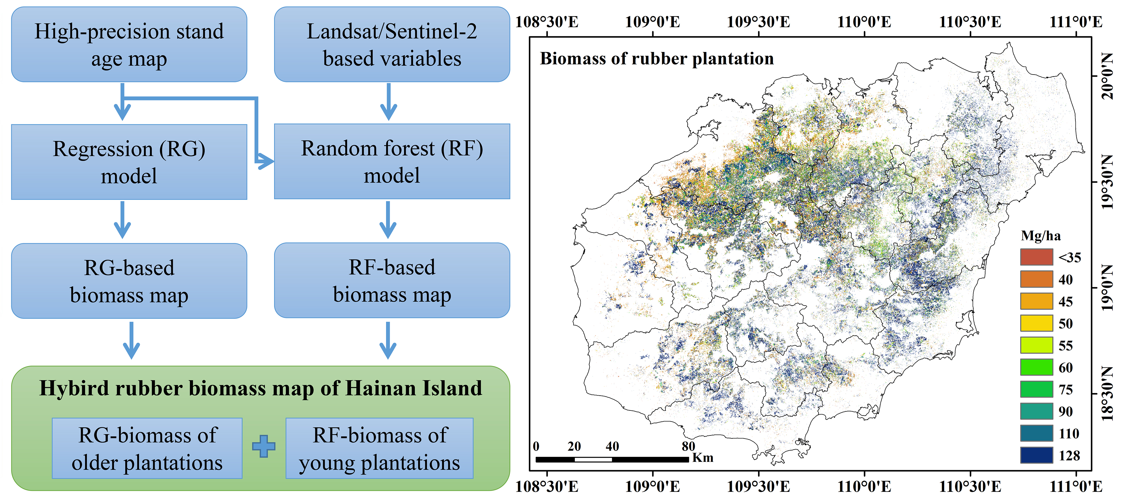
2.1. Study Area

Hainan Island (19°20′N–20°10′N, 108°21′E–111°03′E, Figure 1) is the second largest island in China and has an area of about 3.4 million ha. The topography of the island is mountainous in the interior, with lowlands along the coast. Wuzhi Mountain (1867 m AMSL) is the highest mountain on the island [44]. The climate varies from tropical to subtropical. The annual mean temperature is approximately 23–25 °C, and the monthly temperature varies between approximately 16 °C in January and approximately 30 °C from May to July. The average annual precipitation is 1500 to 2000 mm, about 80% of which occurs during the rainy season from May to October. However, the spatial distribution of precipitation can be as high as 2400 mm in the central and eastern area and as low as 900 mm in the coastal areas of the southwest [45].
Hainan Island is the second largest rubber plantation base in China. In the 1950s, a large area of rubber trees was planted to meet China’s national defense and economic needs. Statistics indicate that Hainan Island had about 5.43 × 10⁵ ha of rubber plantations by the end of 2017, accounting for more than a quarter of the total forest area, and is the largest plantation ecosystem there [44].

2.2. Data and Processing

2.2.1. Field Inventory Data

Field data consist of two parts: the main field data sampled in 2016 and supplementary data derived from [38] or collected from the experimental farm of the Chinese Academy of Tropical Agricultural Sciences (CATAS) from 2007 to 2014. The main field data are new and have a uniform acquisition time, so are used to explore the relationship between rubber biomass and remote sensing variables, to develop Random Forest (RF) models, and to evaluate their accuracy. Both the main field data and supplementary data were used to fit a biomass model using the stand age as the independent variable. The supplementary data were mainly collected for increasing samples in the 1990s—a period established with limited rubber plantations, which made it difficult to acquire wealthy field data by random sampling.
The main field data were collected in October of 2016 by randomly selecting rubber plantations with the aid of Google high-resolution satellite images. In each plantation, the DBH of each rubber tree at a 1.3 m height in an area of 25 × 25 m was measured, and the mean and standard deviation of the DBH were calculated. The stand age was obtained by interviewing farmers or was evaluated according to the height of tapped bark—a relatively fixed height of bark is consumed each year for latex harvest—and double checked with the plantation establishment year map of 2017 (described in Section 2.3). Field photos were taken by a Casio EX-H20G camera embedded with a Global Positioning System (GPS) receiver. The GPS information of the photos was extracted using these steps: (1) converting it into a Keyhole Markup Language (KML) file format by PhotoKML (v1.3) (https://www.softpedia.com/get/Multimedia/Graphic/Graphic-thers/PhotoKML.shtml), (2) importing the KML file in ArcGIS (v10.2, www.esri.com) and converting it into a shapefile format, and (3) extracting the latitude and longitude of each plot. A total of 51 rubber plantations were collected during the field campaign. The spatial distribution of field plots is shown in Figure 1 and descriptive statistics on the stand age and DBH are presented in Table 1. Among the 18 counties where rubber trees have been cultivated, 16 of them have sampling plots.
The DBH and stand age of rubber plantations included in the supplementary data were collected in a similar way, but accurate GPS information of some plantations was not clear. Actually, the stand age is the primary concern when building a stand age-based biomass model. The supplementary data consist of 19 rubber plantations with different stand ages. The total biomass (below + aboveground) for a single rubber tree was calculated by the AE model (Equation (1)) [13]:
ln B G _ t r e e = 2.4021 ln G 4.5803
where B G _ t r e e is the biomass (kg/tree) and G is the girth at 1.3 m (cm). This model has a good accuracy (R2 = 0.99, systematic error ≤ 1.469% [13]). On Hainan Island, rubber trees were generally planted at a density of 3 × 7 m or 4 × 5 m in columns and rows, resulting in about 495 trees/ha at the initial stage of plantation establishment. However, the tree density decreased with the year because of typhoons, which frequently hit the island and caused huge damage in the rubber industry [46]. Tree density data of more than 80 state farms (not distinguishing the stand age), from 1952 to 2001, were collected by Hainan State Farm Bureau [47], showing an average density of 381.45 trees/ha. Equation (1) was converted into Equation (2) at a hectare scale by multiplying the average tree density and by dividing it by 1000 (converting kg to Mg):
B G = 3.9105 G 2.4021 · 10 - 3
where B G is the biomass (Mg/ha). The girth and biomass of each plantation were stored in the attribute table of the shapefile. According to the size of biomass, the field data were split into eight groups (30, 40, 50, 60, 70, 80, 110, and 140 Mg/ha), which were further used as parameters for stratified k-fold cross-validation. Stratified k-fold cross-validation is similar to k-fold cross-validation, but it conducts stratified sampling instead of random sampling to ensure that relative class frequencies are approximately preserved in each train and validation fold. Then, the shapefile was uploaded to the Google Earth Engine (GEE, https://earthengine.google.com/) platform for subsequent analysis and modeling.

2.2.2. Satellite Imagery

Landsat 7/8 and Sentinel-2 multispectral imagery was used in this study. Landsat 7 Enhanced Thematic Mapper Plus (ETM+) and Landsat 8 Operational Land Imager (OLI) imagery were obtained from the U.S. Geological Survey (USGS, www.usgs.gov), and the Sentinel-2 MultiSpectral Instrument (MSI) imagery was obtained from the European Space Agency (ESA, https://sentinel.esa.int). All the top-of-atmosphere (TOA) reflectance data of Landsat 7/8 collection 1 Tier 1 and Sentinel-2 Level-1C were acquired during the day of year (DOY) between 120 and 330 (April 1 to November 30) and from 2016 to 2017. Surface Reflectance (SR) data were not used because Sentinel-2 SR (Level-2A) for the study area was not available at the GEE platform when we first carried out this study, and the mix use of Sentinel-2 TOA and Landsat SR may have the problem of cross-calibration between different sensors. Landsat 7/8 data have a 30-m spatial resolution, and Sentinel-2 MSI has a 10-m spatial resolution. These TOA reflectance data had already been orthorectified with a high geometric accuracy and reduced radiometric uncertainties between different acquisition dates and different sensors, such as ETM+ and OLI. All these data were available on the GEE cloud computing platform and could be readily accessed.
The cloud and cloud shadow of Landsat ETM+ and OLI were masked using bitmask information from the associated quality assessment band, which was generated by the widely used C Function of Mask (CFMask) algorithm [48]. Google’s cloudScore algorithm, together with the Temporal Dark Outlier Mask (TDOM), were used for masking the cloud and shadow of Sentinel imagery [49,50]. Regression models [50] were used to minimize TOA reflectance differences among the sensors of Sentinel-2 MSI, Landsat 7 ETM+, and Landsat 8 OLI, using Landsat 8 OLI TOA reflectance as a benchmark.
A median value composite (similar to a maximum value composite [51], but the median value in each band over time was selected) was applied to Landsat 7/8 and Sentinel-2 (LS2) to generate 20-m resolution cloud-free imagery. Then, two commonly used vegetation indices—the Normalized Difference Vegetation Index (NDVI) [52] and Enhanced Vegetation Index (EVI) [53]—were calculated using Equations (3) and (4), respectively:
NDVI = ρ NIR ρ red ρ NIR + ρ red
EVI = 2.5 × ρ NIR ρ red ρ NIR + 6 × ρ red 7.5 × ρ blue + 1
where ρ blue   , ρ green , ρ red , and ρ NIR are the blue, green, red, and near-infrared (NIR) bands of the composite image (Table 2). Previous studies indicated that principal component analysis (PCA) of Landsat images had stronger relationship with forest biomass than individual bands [31]. Therefore, PCA was computed based on the LS2 composite image.

2.2.3. Terrain Data

The Shuttle Radar Topography Mission (SRTM) digital elevation data (V3) at a resolution of 1 arc-second (approximately a 30-m spatial resolution) were provided by the National Aeronautics and Space Administration (NASA) Jet Propulsion Laboratory (JPL) [54]. The elevation was directly obtained from SRTM V3 data, and the corresponding slope was calculated using GEE’s Application Programming Interface (API).

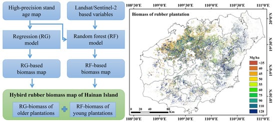
2.3. Rubber Plantation Biomass Estimation

Most AE biomass models are built on DBH, H, or their combination [12,13]. However, the biomass of rubber plantations also displays a close relationship with stand age—the R2 of the established biomass model exceeds 0.93 [8,18]. A stand age-based biomass model is more popular in the remote sensing community because the stand age can be estimated more accurately by dense time-series satellite images than DBH or H [3,43], which are more easily and precisely obtained on the ground. In addition to the stand age, factors such as geography and climatic will affect the growth, meaning that rubber plantations of the same age have different canopy characteristics and biomasses. We made a hypothesis that integrating the stand age and spectral signatures from satellite imagery acquired in the growing season (April to December) can improve the estimation accuracy of the biomass model. Two methods were used to estimate the biomass of rubber plantations, and their differences were compared. The first was a regression model solely fitted by stand age, and the second was a Random Forest (RF) model built on LS2-based variables and/or the stand age. To generate a wall-to-wall biomass map of Hainan Island, both models require a reliable stand age map of rubber plantations in advance.

2.3.1. Mapping the Stand Age of Rubber Plantations

In a previous study, we developed a new algorithm to identify the establishment year (same as the stand age, where the stand age equals the target year minus the establishment year) of rubber plantations based on all Landsat images of Hainan Island [3]. Specifically, signatures that topsoil exposed during plantation establishment and canopy closure linearly increased during nonproductive periods (rubber seedling to mature plantations) were employed to identify the establishment year. Annual images of the minimum and average Land Surface Water Index (LSWI) from 1987 to 2015 were respectively composited from all Landsat images (about 2000 scenes in total) acquired in the growing season of the corresponding year and were then used to generate an establishment year map of rubber plantations for Hainan Island in 2015. The establishment year map at an annual resolution since 1987 shows a very high accuracy (R2 = 0.85/0.99 and RMSE = 2.34/0.54 year at a pixel/plantation scale). The establishment year established before 1987 was uniformly set as 1986 because the earliest collection of Landsat 5 imagery of Hainan Island started in 1987. We used the same algorithm and thresholds to generate the stand age map in 2017, using the newly obtained map of rubber plantations in 2017 as a benchmark and adding annual composited images of 2016 and 2017 to the previous annual composited data set.

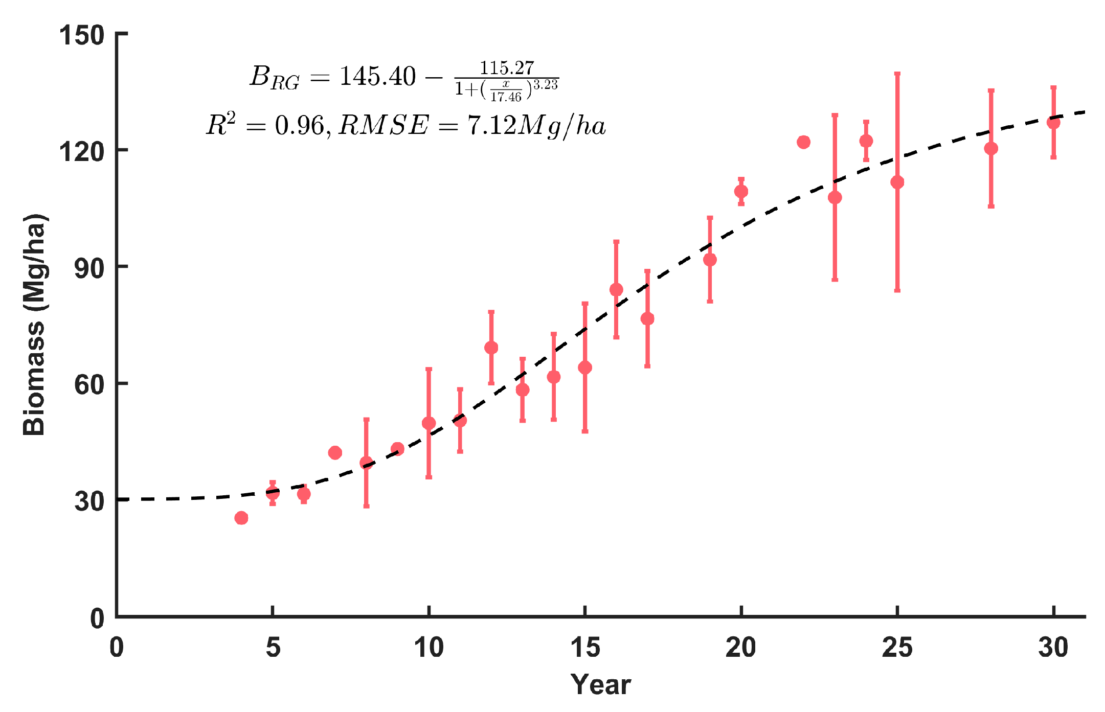
2.3.2. Regression Biomass Model

Both the main field data (51 plots) and supplementary field data (19 plots) were used to build a regression biomass model. The field data used were obtained from rubber plantations of less than 30 years old. It is difficult to accurately obtain a stand age of over 30 years from both remote sensing and ground surveys—the former case is because of a lack of time-series images for mapping (the earliest collection of Landsat 5 images of Hainan Island began in 1987), while the latter case is due to difficulties in determining the stand age from blurred tapping bark of old trees. The biomass was grouped according to stand age, and their average and standard deviation values were calculated. The stand age was used as the independent variable, and the average biomass was the dependent variable. An “S”-shaped sigmoidal biomass model was built using an online curve-fitting utility named MyCurveFit (mycurvefit.com). The biomass estimated by the regression model was referred to as B R G .

2.3.3. Random Forest (RF) Biomass Model

The RF machine learning algorithm is generally immune to data noise and overfitting [55] and has been widely used within the remote sensing community such as classification [56,57,58,59], biomass estimation [25,60], disease monitoring [61,62], and hazards detection [63]. The good performance of the RF model over other methods, such as maximum likelihood and single decision trees, has been demonstrated by many studies and was summarized by Belgiu et al. [64].
Three tests were conducted during RF model building: (1) biomass saturation (sensitivity to biomass is lost up to a point) with different variables from LS2 composite images, (2) model building using LS2-based variables, and (3) model building using LS2-based variables and the stand age. Based on previous studies on forest biomass [31], we selected variables such as B3, B4, B5, B7, PC1, PC2, PC3, NDVI, and EVI to construct an independent variable data set. A scatter plot and the Pearson correlation coefficient between different variables and biomass were used to assess the biomass saturation. We calculated multiple correlation coefficients using samples of different biomass sizes, starting from 40 Mg/ha, with 5 Mg/ha as the step until 80 Mg/ha.
Every possible variable combination by gradually adding a distinct variable from the independent variable set—B3 and B4, and B3 and B5 as combination examples—was used to build RF models. We also tested the model performance under conditions of with/without stand age as a fixed independent variable. We kept the best 10 RF models each time and finally compared their performance under different variable combinations. Considering the problem of biomass saturation, model building was also conducted for samples from different biomass groups (smaller than mean values of 50, 60, 70, 80, 110, and 140 Mg/ha, respectively). Due to the limited sample size, we did not perform model testing on samples with a biomass of less than 50 Mg/ha, even using k-fold cross-validation (K = 4 was used here). In order to improve the efficiency of the test, we downloaded the sample data containing LS2-based variables from GEE to a local computer and then used the scikit-learn (https://scikit-learn.org/stable/index.html) python package for model testing. The number of trees in the forest was set as 100 and random_state was set as 1. The biomass estimated by the RF model was referred to as B R F .

2.4. Accuracy Assessment

Stratified k-fold cross-validation (StratifiedKFold) was used to evaluate the model accuracy. The 51 samples were split into four smaller sets (each set is called a fold) using grouping field (values close to 30, 40, 50, 60, 70, 80, 110, and 140 Mg/ha) for stratification. The model was trained using k-1 of the folds as training data and was validated with the remaining part. The performance measure reported by k-fold cross-validation was then the average of the values computed in the loop. Model performances were evaluated by the determination of coefficients (R2) and Root Mean Square Error (RMSE). The scatter of B G against B R G and B R F was plotted, respectively. Matplotlib (https://matplotlib.org) and Seaborn, which is a Python data visualization library based on matplotlib (https://seaborn.pydata.org), were used for plotting.

3. Results

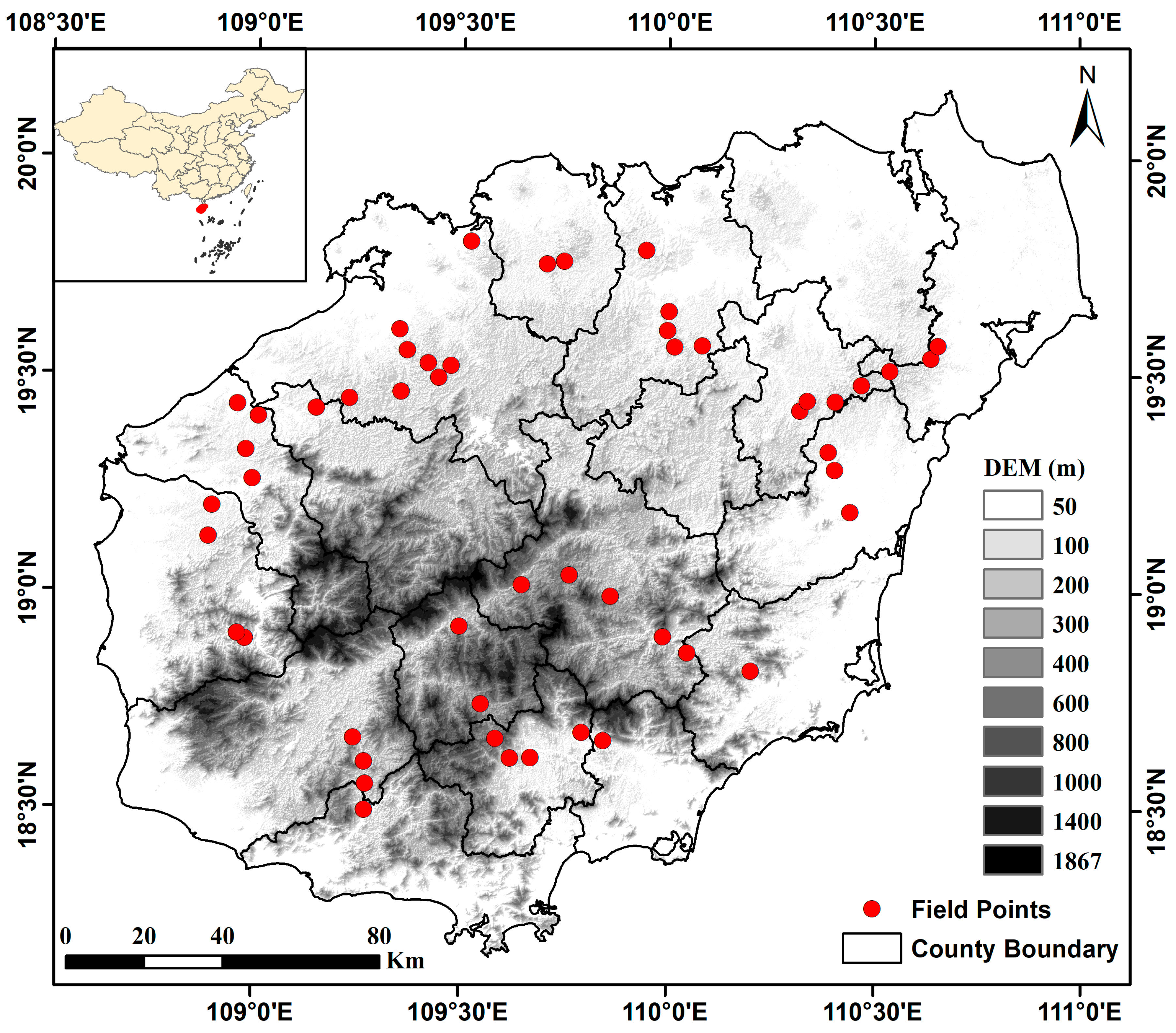
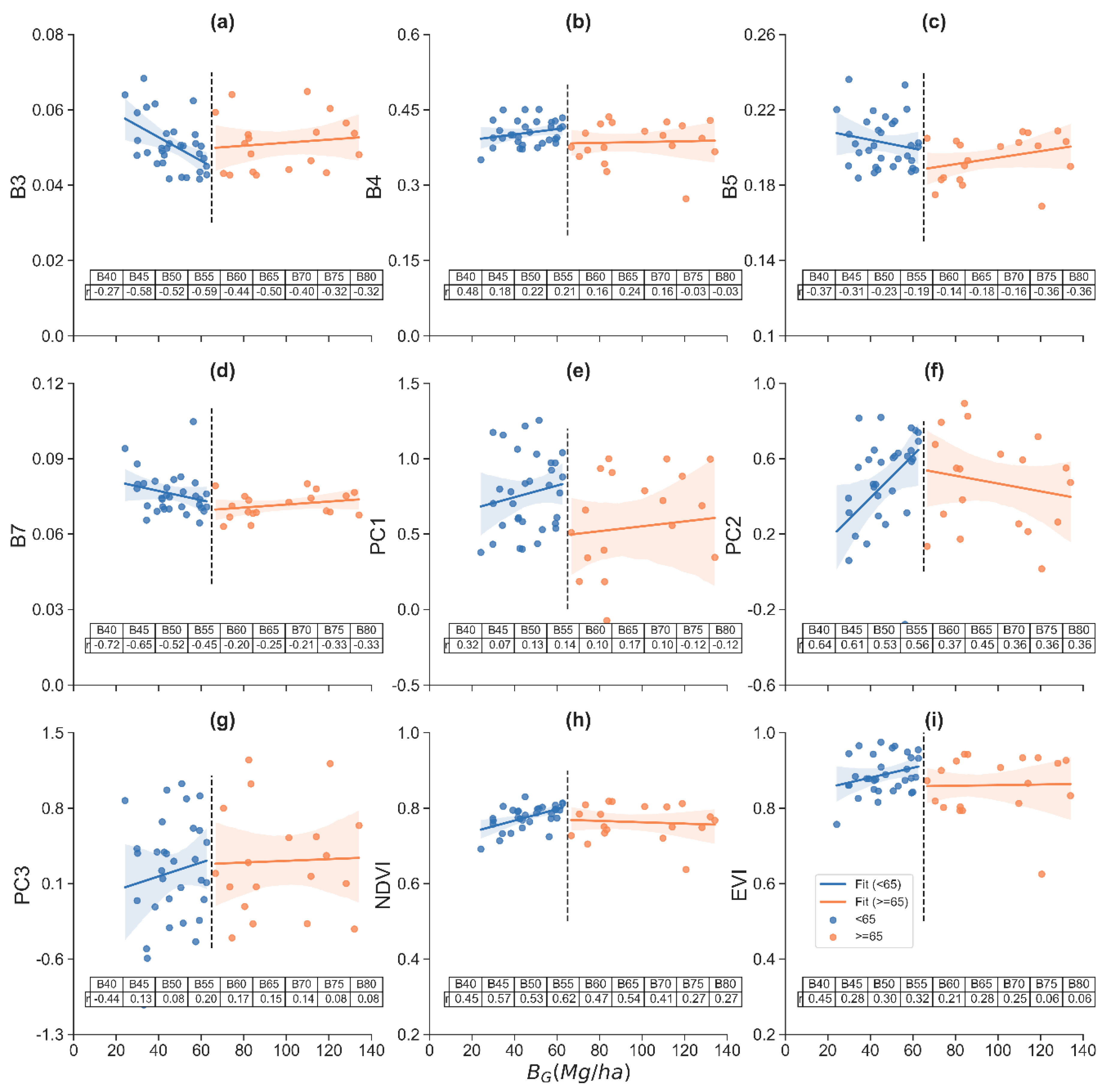
3.1. Variable Sensibility to the Biomass of Rubber Plantations

The scatter plots and correlation coefficients of biomass against different spectral bands, vegetation indices, and principal components are presented in Figure 2. The reflectance of B3, B5, and B7 decreases with biomass when the biomass is lower than 65 Mg/ha and then increases slowly. Among them, B3 drops more significantly, followed by B7 and B5. PC1, PC2, PC3, NDVI, and EVI first increase with the increase in biomass, but there are almost no changes after the biomass is greater than 65 Mg/ha, except for PC2, showing an obvious decrease in a high biomass range. The relationship between B4 and biomass is the weakest, even if the biomass is divided into two parts at 65 Mg/ha. When the biomass is lower than 65 Mg/ha, its correlation coefficient with B3, B7, PC2, and NDVI is quite high among these variables, ranging from −0.27 to −0.59, −0.20 to −0.72, 0.37 to 0.64, and 0.45 to 0.62, respectively. When the biomass continues to increase, the correlation coefficient between it and all variables weakens.

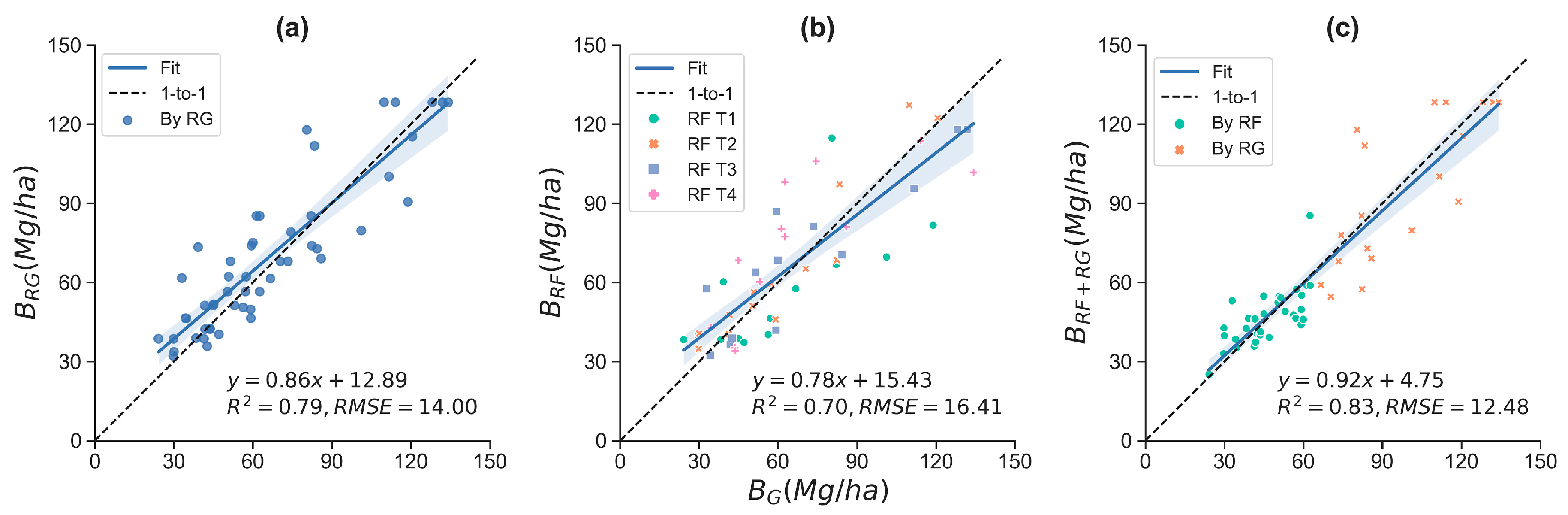
3.2. Biomass Estimated by the Regression Model

A nonlinear symmetrical sigmoidal model, named the four parameter logistic (4PL) regression model, was used to establish a regression model between the biomass of rubber plantations and stand age (Equation (5), 95% confidence) (Figure 3):
B R G = 145.40 115.27 1 + ( x 17.46 ) 3.23
where B R G is the biomass of rubber plantations (Mg/ha) and x is the stand age. The R2 is 0.963, adjusted R2 is 0.967, RMSE is 7.12 Mg/ha, and Sum of Square Error (SSE) is 911.12. A slight overestimation is observed in immature plantations for which the stand age is less than 5 years. The maximum biomass for this model is about 145.40 Mg/ha. When combined with the biomass model and latest stand age map, the biomass of rubber plantations on Hainan Island could be obtained. Validation by main ground reference data collected in 2016 shows that R2 reaches 0.79 and that RMSE is 14.00 Mg/ha (Figure 4a). The scatter plot of B R G against B G demonstrates that most points distributed along the 1-to-1 line, but the model exhibits a slight overestimation when rubber biomass is less than about 80 Mg/ha (Figure 4a).

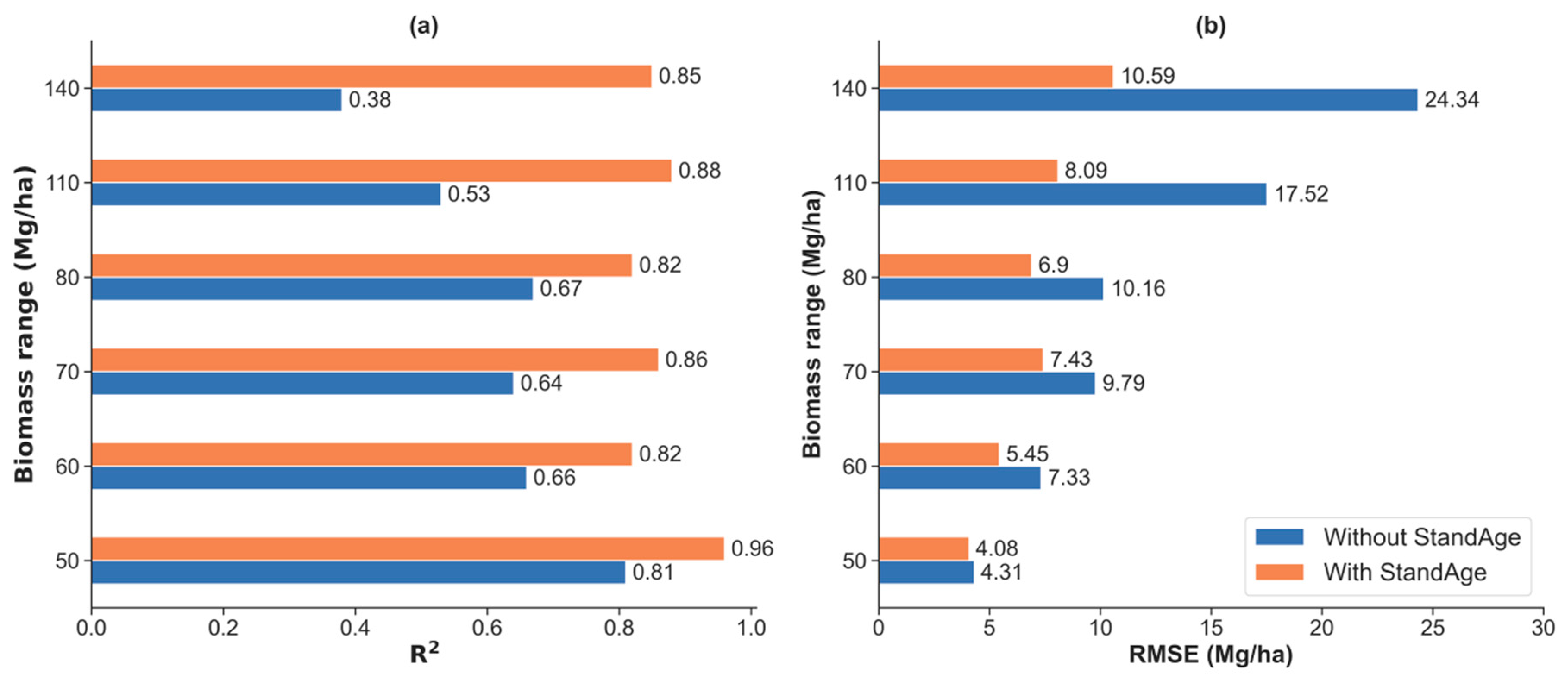
3.3. Biomass Estimated by RF Models

R2 of the best RF models developed by variable combinations of B3, B4, B5, B7, PC1, PC2, PC3, NDVI, and EVI ranges from 0.38 to 0.81, and the RMSE is between 4.31 and 24.34 Mg/ha (Figure 5). The RF model trained with samples of less than or equal to group 50 (specifically, all samples with a biomass < 55 Mg/ha) holds the highest R2 (0.81) and lowest RMSE (4.31 Mg/ha). R2 decreases to about 0.65 when sample groups less than 60, 70, and 80 are used for modeling and then gradually decreases to about 0.38 when the samples of a higher biomass (groups 110 and 140) are added to the models. However, the RMSE of the RF models generally increases from 4.31 to 24.34 Mg/ha with the addition samples of a higher biomass.
When the stand age is a fixed independent variable, the prediction accuracies of RF models are significantly improved. R2 ranges from 0.81 to 0.96, and the RMSE is between 4.08 and 10.59 Mg/ha (Figure 5). The accuracy of the RF model built with samples of less than and equal to the 50 group is the highest, where R2 reaches 0.96 (0.15 higher than that without using the stand age) and RMSE drops to 4.08 Mg/ha. When the sample biomass is high, the increase in R2 is more obvious. For example, R2 of a model built with samples of less than or equal to the 140 group increases from 0.38 to 0.85 and the RMSE decreases from 24.34 to 10.59 Mg/ha. The RMSE of the RF models generally increases with the addition of higher biomass samples.
The scatter plot of the best RF model developed by stand age and LS2-based variables with k-fold cross-validation is shown in Figure 4b. The points are more densely distributed near the 1-to-1 line when the biomass of rubber plantations is less than about 65 Mg/ha, and most points are then more scattered afterwards. The R2, RMSE, and slope of the fit line are 0.70, 16.41 Mg/ha, and 0.78, respectively. A slight underestimation is observed for plantations which exhibit a higher biomass.
Since the RF models have a higher prediction accuracy for plantations with a lower biomass (Figure 5) and the regression model presents a high accuracy for plantations with a higher biomass (Figure 4a), a hybrid model integrating the optimal results of these two models can better predict the accuracy. The scatter plot of B G against results obtained from the hybrid model (BRG + RF) is shown in Figure 4c. The prediction results are more closely distributed around the 1-to-1 line. The slope of the fit line, R2, and RMSE are 0.92, 0.83, and 12.48 Mg/ha, respectively.

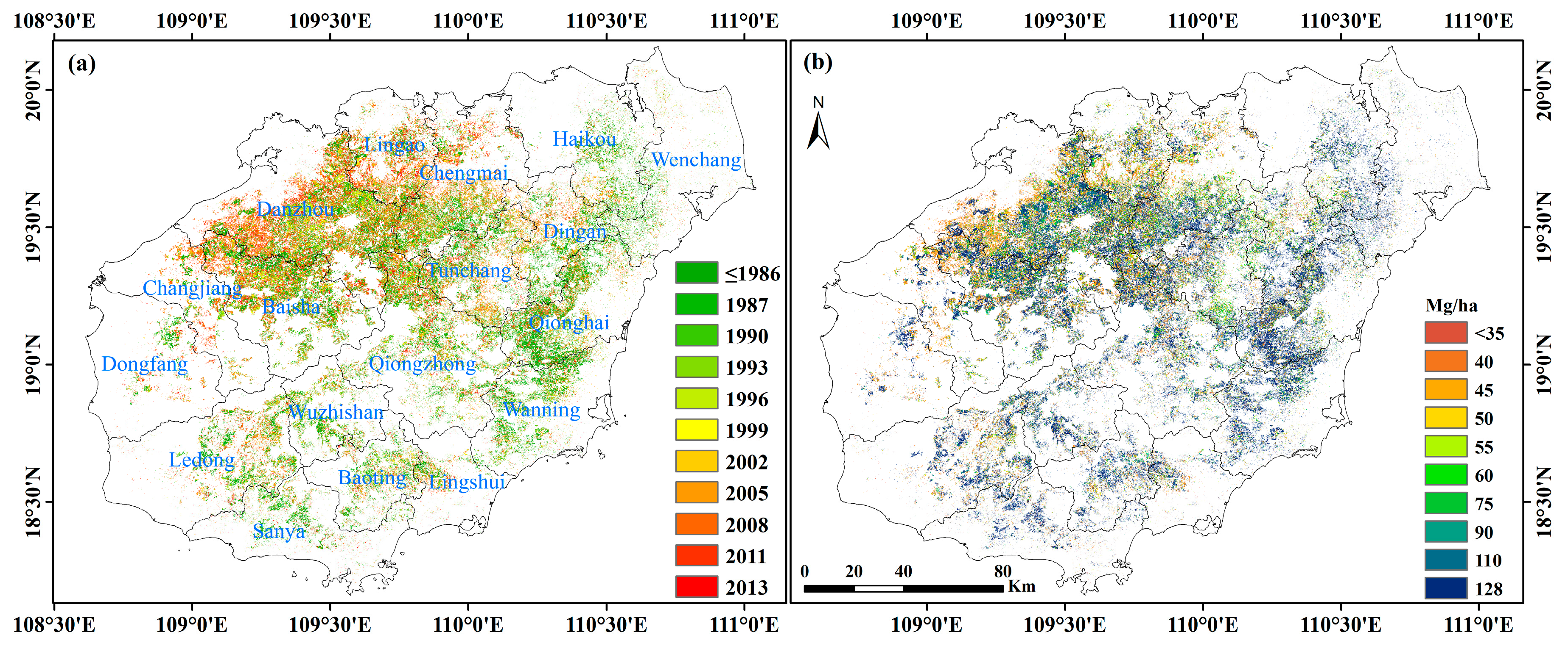
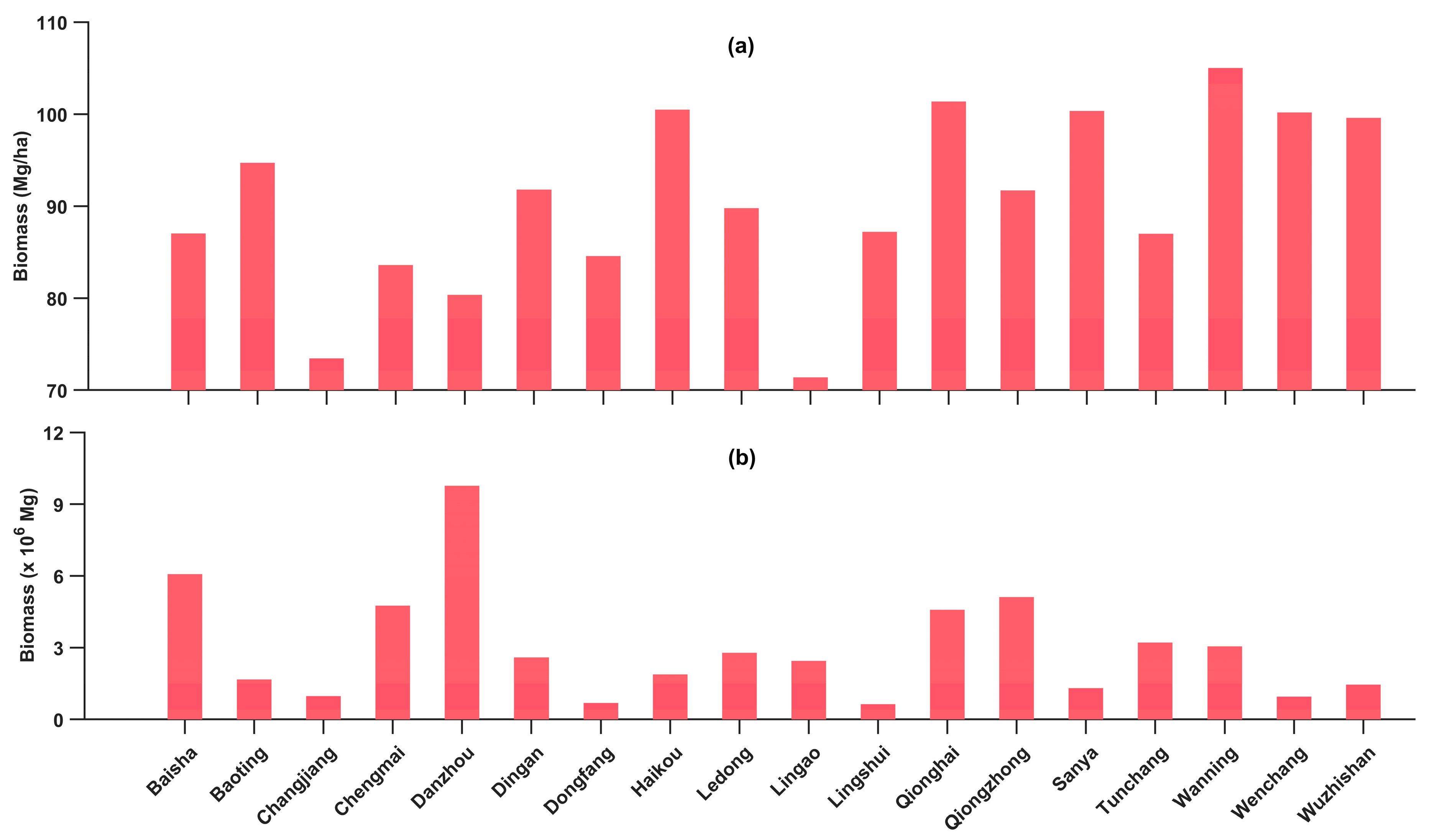
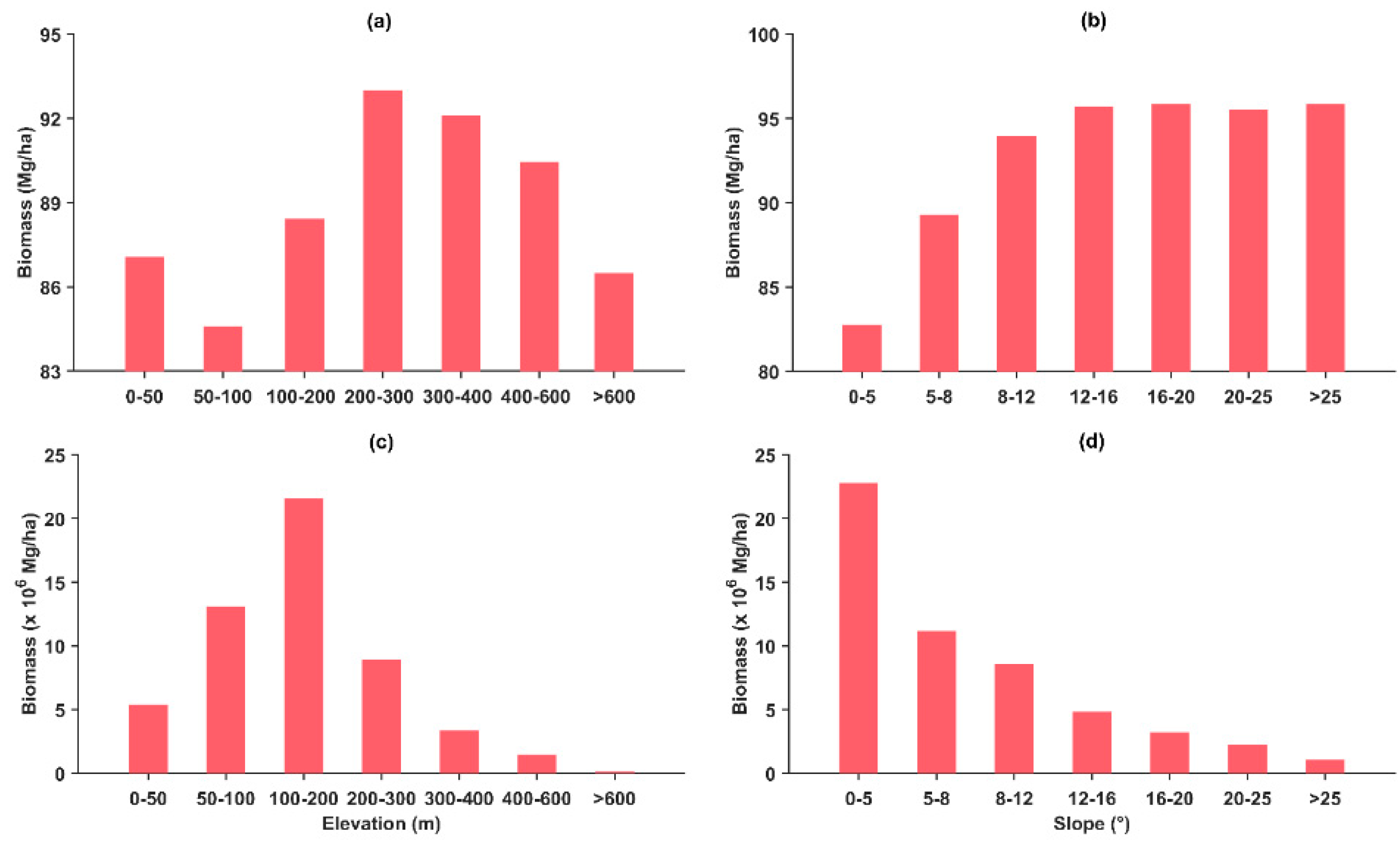
3.4. The Spatial Distribution of Rubber Plantations and Biomass

The establishment year map of rubber plantations on Hainan Island by the end of 2017 is shown in Figure 6a. Immature plantations with a stand age of less than four years were excluded from this map because of larger mapping uncertainties. Rubber plantations are densely distributed in northern and center-to-east regions. Danzhou city possesses the largest area of rubber plantations, whilst other counties, such as Baisha, Chengmai, Qiongzhong, and Qionghai, also have dense distributions. The establishment year map shows an interesting distribution: A considerable number of rubber plantations have been established in the western and northern regions since 2000, whereas the old rubber plantations are mainly distributed along the coastal strip from south to northeast.
The spatial distribution of the biomass of rubber plantations generated by the hybrid model is shown in Figure 6b. The spatial distribution pattern is quite consistent with the spatial distribution of the establishment year. The biomass of newly established rubber plantations in the western and northern regions is generally below 60 Mg/ha, while the biomass of aging plantations distributed along the coastal strip from south to northeast and some border regions such as Danzhou city and Baisha county usually exceeds 110 Mg/ha. The biomass of some rubber plantations discretely distributed in Danzhou city and counties of Baisha and Qiongzhong is greater than 90 Mg/ha.
The average biomass of rubber plantations varies in different counties or cities (Figure 7a). Wanning city possesses an average biomass of about 105 Mg/ha and tops the rankings, followed by the cities of Qionghai, Haikou, Wenchang, Sanya, and Wuzhishan, all of which have an average biomass of about 100 Mg/ha. Baoting county has an average biomass of about 95 Mg/ha, followed by the counties of Dingan, Qiongzhong, and Ledong, possessing an average biomass that is slightly greater than 90 Mg/ha. The average biomass of Danzhou city, representing the largest production base on Hainan Island, is about 80 Mg/ha. Changjiang and Lingao county exhibit the lowest values among the 18 counties or cities, displaying an average biomass of about 72 Mg/ha.
The total biomass of rubber plantations varies dramatically among different counties or cities (Figure 7b). Danzhou city possesses a total biomass of 9.77 × 10⁶ Mg, which is far higher than other counties or cities, followed by the counties of Baisha, Qiongzhong, Chengmai, and Qionghai city, all of which have a total biomass of rubber plantations greater than 4.50 × 10⁶ Mg. The total biomasses of rubber plantations in Tunchang county, Wanning city, Ledong county, Dinan city, and Lingao county are about 3.21 × 10⁶, 3.05 × 10⁶, 2.78 × 10⁶, 2.59 × 10⁶, and 2.45 × 10⁶, respectively, while the remaining counties or cities have values of less than 2.00 × 10⁶ Mg. Dongfang city and Lingshui county have the smallest biomass of rubber plantations, possessing values of 6.88 × 10⁵ and 6.37 × 10⁵ Mg, respectively. The total biomass of rubber plantations on Hainan Island in 2017 was 5.40 × 10⁷ Mg.
The average biomass of rubber plantations varies greatly at different elevations and slopes (Figure 8a,b). The highest average biomass is located at an elevation between 200 and 300 m, which is about 93 Mg/ha, followed by rubber plantations distributed in an elevation range from 300 to 400 m and from 400 to 600 m. The lowest average biomass is located at an elevation between 50 to 100 m, which is about 85 Mg/ha. In areas with a slope below 12 degrees, the average biomass of rubber plantations increases with an increase in the slope, gradually increasing from about 83 Mg/ha within five degrees to about 94 Mg/ha at regions of 8–12 degrees. After the slope exceeds 12 degrees, the average biomass of rubber plantations is maintained at about 96 Mg/ha.
The total biomass of rubber plantations on Hainan Island is mainly distributed in low elevation and flat areas (Figure 8c,d). At an elevation of 100 to 200 m, the total rubber biomass is the highest, exceeding 2.16 × 10⁷ Mg, followed by areas of 50 to 100 and 200 to 300 m, with values of about 1.31 × 10⁷ Mg and 8.95 × 10⁶ Mg, respectively. The total biomass in areas above a 600-m elevation is extremely low. The total biomass of rubber plantations gradually decreases with an increasing slope. In flat areas of less than five degrees, the total biomass is close to 2.28 × 10⁷ Mg, followed by areas of 5–8 degrees, for which the total biomass is 1.12 × 10⁷ Mg.

4. Discussion

4.1. Biomass Saturation with Different LS2-Based Variables

Many studies have reported that the saturation point between the biomass of rubber plantations and different variables from remote sensing was very low. In this study, the saturation point of rubber plantations with B3, B4, B5, B7, PC1, PC2, PC3, NDVI, and EVI from LS2-based composite images was about 65 Mg/ha, which was higher than in studies conducted in Cambodia [36] and Thailand [2]. Avtar et al. [36] found that the PALSAR HV band positively correlated with the aboveground biomass of rubber plantations but was saturated at 50 Mg/ha. Yasen and Koedsin [2] found that the aboveground biomass of rubber plantations was saturated with WorldView-2 images at 40 Mg/ha in Phuket Province, Thailand. The main reason for the higher saturation point we monitored was that it contains belowground biomass. If the underground biomass was deducted at a rate of 20% [13], the saturation point of the aboveground biomass was also around 50 Mg/ha, which was consistent with these studies. Since the most LS2-based variables were saturated when the rubber biomass was very low, it was difficult to accurately estimate the biomass of rubber plantations from these variables. For example, only one model we developed using samples less than 55 Mg/ha had an R2 of 0.81. The R2 of other models built on samples with a biomass of less than 85 Mg/ha was about 0.65 and decreased to 0.38 when all samples were used for modeling (Figure 5a).

4.2. Biomass Estimation Using Stand Age and Remote Sensing Parameters

The regression biomass model fitted by stand age had a high accuracy (R2 = 0.96 and RMSE = 7.12 Mg/ha), which was consistent with previous studies [8,10,18]. The high accuracy of the model could be explained by the fact that rubber plantations have a shorter economic life cycle (about 25–30 years). The growth of biomass only became slow after more than 20 years [38], so the biomass had a close relationship with stand age. The maximum biomass from this regression model (145.40 Mg/ha) was similar to studies such as [9,65], reporting 63.70 and 65.10 Mg C/ha of carbon stock for rubber plantations with rotation periods of 38 and 25 years, respectively. However, this value was much higher than the value from Trisasongko’s model—the maximum biomass of a 30-year-old rubber plantation was about 70 Mg/ha [37]. In addition to stand age, the planting density also affects biomass accumulation greatly [10]. We have incorporated planting density in the regression model, according to 50 years of extensive surveys from Hainan State Farm Bureau.
Obtaining a high-precision stand age map was essential for estimating the biomass of rubber plantations over a large area. Currently, most studies use one or several satellite images to estimate stand age, obtaining a stand age map of different age groups (e.g., <7, 5–15, and >15) [66,67,68]. In this study, the stand age map of rubber plantations in 2017 was generated at annual steps using all LS2 images acquired from 1987 to 2017 and a novelty algorithm developed in a previous study [3]. With this reliable stand age map, the biomass map through the regression model of Hainan Island exhibited high accuracy (R2 = 0.79 and RMSE = 14.00 Mg/ha), better than models without the stand age—for example, higher than the regression model (R2 = 0.43) developed in Cambodia [36]; artificial network model (R2 = 0.66 and RMSE = 11.97 Mg/ha) established in Phuket Province, Thailand [2]; and RF model (R2 = 0.43 and RMSE = 34.05 Mg/ha) built in Xishuangbanna, Yunnan Province, China [34]. Using an accurate stand age map and models, the wall-to-wall biomass map could be obtained. Theoretically, this method was superior to the traditional BCEF approach since it was difficult to establish a yearly scale conversion factor [14].
In addition to the stand age, signatures from satellite images contributed to the improvement of biomass estimation. However, the model built based on all samples had a large estimation bias especially in plantations which have higher biomass (Figure 4b) because the biomass of rubber plantations was saturated at around 65 Mg/ha (Figure 2). Previous research also found a similar estimation bias. For example, Yasen and Koedsin [2] found that the artificial neural network model was seriously underestimated after the biomass of rubber plantations exceeded about 50 Mg/ha, and Wang et al. [34] found that the stepwise regression model showed severe underestimation after 200 Mg/ha. The estimation bias issue in the RF model could be solved by replacing the prediction results of aging plantations (biomass of over 65 Mg/ha) with corresponding results from the regression model (estimated solely by stand age). R2 of the hybrid model was improved from 0.79 to 0.83, and the RMSE was decreased from 14.00 to 12.48 Mg/ha (Figure 4b).
RF was widely used and proven to have a higher prediction accuracy than other algorithms because of its many advantages, such as the fact that it is not sensitive to noise or overtraining and requires less computational resources [69]. In this study, RF also showed a high prediction accuracy. For example, the R2 of RF models developed with samples of biomass less than 85 Mg/ha and LS2-based variables reached about 0.65, although the biomass of rubber plantations was saturated at about 65 Mg/ha. However, as reported in previous studies [64], the RF model was also very sensitive to the sample design. Initially, we randomly divided the samples into training and validation sets, but the estimation accuracy was quite low because sample sizes of different age groups varied greatly. After we adopted the stratified k-fold cross-validation method, the accuracy and stability of the RF models improved greatly since more samples could be used for modeling and cross-validation. In addition, cross-sensor calibration among LS2 images also promoted high accuracy of RF models since the differences in band values among MSI, ETM+, and OLI were significant for all cross-sensor band pairs [50]. In the future, more data sources, such as PALSAR-2 radar data, and more influence factors, such as the altitude and slope, can be included to further improve the prediction accuracy of the models. For example, terrain factors affect not only the light and temperature environment of the forest plantations but also the signal strength of remote sensing, which is used for modeling [22].

4.3. Biomass of Rubber Plantations on Hainan Island

Rubber plantations account for more than one fourth of the total forest area on Hainan Island and are the largest forest plantation ecosystem there. Therefore, it is of vital importance to evaluate their biomass at a province scale. The average rubber biomass for the island is 90.53 Mg/ha, which is higher than the 83.25 Mg/ha [33] and 75.90 ± 58.75 Mg/ha [32] values estimated in Xishuangbanna, Yunnan Province, China. The main reason for the higher average biomass is the introduction of stand age during model building, which greatly reduced the signal saturation problem commonly encountered in the remote sensing community. The average rubber biomass was smaller than 108.35 ± 11.48 Mg/ha in 14-year-old plantations at a low elevation but higher than 79.71 ± 14.48 Mg/ha in plantations of the same age at a medium elevation in Xishuangbanna, Yunnan Province, China [12].
Since many rubber plantations were established after 2003, the biomass density in the northern and western areas of Hainan Island was relatively low and was mostly less than 75 Mg/ha (Figure 6). Danzhou city, which is the largest rubber production base on Hainan Island, is mixed with plenty of young and aging rubber plantations, leading to a higher average biomass (about 80 Mg/ha) than that of Lingao county (about 71 Mg/ha, representing the lowest average biomass), where most rubber plantations were established after 2003 (Figure 7). The highest biomass density along the coastal strip from south to northeast (e.g., the average biomass in the cities of Sanya, Wanning, Qionghai, and Wenchang is about 100 Mg/ha, Figure 7) can be explained by the large number of aging rubber plantations there. It was previously found that farmers were no longer willing to plant rubber trees in these regions, frequently hit by severe typhoons [46,70], even if the natural rubber price was rising rapidly. The expansion trend of rubber plantations in the western and northern areas was very obvious, leading to great changes in the biomass spatial pattern. However, rubber plantations have not expanded to high elevations and steep areas in the past few decades, so the average biomass in areas with a slope higher than 12 degrees has hardly changed, and the total biomass is concentrated in areas 400 m above sea level (Figure 8). Our previous study indicated that a large number of rubber plantations converted from cropland were concentrated in the northwestern part, which has relatively low elevations (Figure 1) and a large amount of flat cropland [3], causing a very low average biomass in low elevation and flat areas (Figure 8). The total biomass of rubber plantations by the end of 2017 was 5.40 × 10⁷ Mg, which is equivalent to 2.70 × 10⁷ Mg carbon if 0.5 is taken as the conversion factor [9].

4.4. Uncertainties in Biomass Estimation on a Large Scale

There are several factors affecting the estimation accuracy of rubber plantation biomass, including the accuracy of the stand age map, landscape fragmentation, and the tree density.

4.4.1. The Accuracy of the Stand Age Map

Although we used all LS2 images and an algorithm based on changes of land use and the biophysical canopy of rubber plantations to generate the stand age map [3], there are still many uncertainties, especially for plantations established before 2000—a stage of acquiring a limited number of images from the Landsat 5 satellite. In addition, the establishment year of rubber plantations established earlier than 1987 was uniformly set to 1986, leading to an underestimation of the stand age and biomass (estimated by the regression model).

4.4.2. Landscape Fragmentation

Due to the strong interference from human activities, rubber plantation patches were quite small and often mixed with different crop patches. The severely fragmented landscape has brought many difficulties to the accurate mapping rubber plantations and their stand age [3]. This is why we used a single pixel instead of the average value of the 3 × 3 pixel window of the field data for modeling.

4.4.3. Tree Density

Due to being frequently affected by severe typhoons, the tree density of rubber plantations on Hainan Island gradually decreases as the stand age increases [46,70]. However, we could not establish a model of the tree density and stand age because of the lack of abundant field data. Instead, a fixed density of 381.45 trees/ha, according to field data collected by Hainan State Farm Bureau, was used to estimate the biomass of rubber plantations. This tree density was smaller than the 418.99 tree/ha value used in Thailand, which is rarely hit by typhoons [9]. Using a fixed tree density underestimates the biomass of young and middle-aged plantations but overestimates the biomass of aged plantations. However, the biomass of rubber plantations established before 1987 was underestimated due to the underestimation of stand age (uniformly set to 1986), which, to some extent, offsets the overestimated biomass of old rubber plantations.

5. Conclusions

Biomass is a crucial variable for estimating the carbon storage capacity and the potential carbon pool size of a forest ecosystem. It is of great importance to estimate the biomass of rubber plantations that are widely distributed in tropical regions. Our results show that the biomass of rubber plantations is closely related to stand age and that R2 of the stand age-based biomass model (regression model) can reach 0.97. When the biomass of plantations is small, they are closely related to the LS2-based variables, especially B3, B7, PC2, and NDVI, and the absolute value of most correlation coefficients is around 0.55. However, the biomass of rubber plantations is saturated with all LS2-based variables at around 65 Mg/ha. Combined with the annual-scale high-precision map of the rubber stand age in 2017 and regression model, the biomass of rubber plantations on Hainan Island was estimated with a satisfactory accuracy (BRG, R2 = 0.79 and RMSE = 14.00 Mg/ha). However, the hybrid model with joint results of regression and RF models has a higher accuracy and low estimation bias (BRG + RF, R2 = 0.83 and RMSE = 12.48 Mg/ha). The introduction of stand age into the models significantly solved the problem of biomass saturation, which occurs at about 65 Mg/ha with satellite-based signatures.
The results showed that there were a large number of rubber plantations with a low biomass distributed in the western and northern areas of Hainan Island, usually below 75 Mg/ha, because of rapid expansion since 2003. High-biomass rubber plantations were mainly distributed in the inner region of the coastal strip from south to northeast, which have frequently suffered from severe typhoons in the past few decades. For example, the average biomass of rubber plantations in Wanning city, southeast of Hainan Island, was close to 105 Mg/ha, ranking top among all cities and counties. Danzhou city, representing the largest rubber production base on Hainan Island, possessed the largest total biomass of 9.77 × 10⁶ Mg, followed by Baisha and Qiongzhong counties. The total biomass of rubber plantations on Hainan Island by the end of 2017 was 5.40 × 10⁷ Mg, indicating a great carbon pool there. The maps of stand age and biomass are of great value for regional carbon budget evaluation and can assist in the development of sustainable management policies to maximize the potential benefits of rubber tree resources.

Author Contributions

Conceptualization: B.C., X.X., and G.X.; methodology: B.C., J.M., and W.K.; software: B.C.; validation: B.C. and C.Y.; formal analysis: B.C. and R.S.; investigation: B.C., J.M., X.Z., and C.Y.; resources: T.Y. and H.L.; data curation: B.C. and X.X.; writing—original draft preparation: B.C.; writing—review and editing: B.C., X.X., and T.Y.; visualization: B.C. and R.S.; supervision: Z.W., W.K., and G.X.; project administration: Z.W.; funding acquisition: B.C., T.Y., W.K., and Z.W. All authors commented on the manuscript. All authors have read and agreed to the published version of the manuscript.

Funding

This research was funded in part by the Natural Science Foundation of Hainan Province (2019RC329), by the National Natural Science Foundation of China (41701510, 31770591, and 31760181), by the Earmarked Fund for China Agriculture Research System (CARS-33-ZP3 and CARS-33-ZP1), and by the Joint Special Project of Agricultural Basic Research in Yunnan Province (2017FG001-034).

Acknowledgments

We thank the U.S Geological Survey (USGS) EROS Data Center and European Space Agency (ESA) for their data sources and Google for their GEE platform.

Conflicts of Interest

The authors declare no conflict of interest.

References

  1. Suratman, M.N.; Bull, G.Q.; Leckie, D.G.; Lemay, V.M.; Marshall, P.L.; Mispan, M.R. Prediction models for estimating the area, volume, and age of rubber (Hevea brasiliensis) plantations in Malaysia using Landsat TM data. Int. For. Rev. 2004, 6, 1–12. [Google Scholar] [CrossRef]
  2. Yasen, K.; Koedsin, W. Estimating Aboveground Biomass of Rubber Tree Using Remote Sensing in Phuket Province, Thailand. J. Med. Bioeng. 2015, 4, 451–456. [Google Scholar] [CrossRef]
  3. Chen, B.; Xiao, X.; Wu, Z.; Yun, T.; Gan, S.; Ye, H.; Lin, Q.; Doughty, R.; Dong, J.; Xiao, X.; et al. Identifying Establishment Year and Pre-Conversion Land Cover of Rubber Plantations on Hainan Island, China Using Landsat Data during 1987. Remote Sens. 2018, 10, 1240. [Google Scholar] [CrossRef]
  4. Carlson, K.M.; Curran, L.M.; Ratnasari, D.; Pittman, A.M.; Soares-Filho, B.S.; Asner, G.P.; Trigg, S.N.; Gaveau, D.A.; Lawrence, D.; Rodrigues, H.O. Committed carbon emissions, deforestation, and community land conversion from oil palm plantation expansion in West Kalimantan, Indonesia. Proc. Natl. Acad. Sci. USA 2012, 109, 7559–7564. [Google Scholar] [CrossRef]
  5. Li, L.; Guo, Q.; Tao, S.; Kelly, M.; Xu, G. Lidar with multi-temporal MODIS provide a means to upscale predictions of forest biomass. ISPRS J. Photogramm. 2015, 102, 198–208. [Google Scholar] [CrossRef]
  6. Thapa, R.B.; Watanabe, M.; Motohka, T.; Shimada, M. Potential of high-resolution ALOS–PALSAR mosaic texture for aboveground forest carbon tracking in tropical region. Remote Sens. Environ. 2015, 160, 122–133. [Google Scholar] [CrossRef]
  7. Zheng, G.; Tian, Q.; Chen, J.; Ju, W.; Xia, X. Combining remote sensing imagery and forest age inventory for biomass mapping. J. Remote Sens. 2006, 10, 932–940. [Google Scholar] [CrossRef] [PubMed]
  8. Tang, J.; Pang, J.; Chen, M.; Guo, X.; Zeng, R. Biomass and its estimation model of rubber plantations in Xishuangbanna, Southwest China. Chin. J. Ecol. 2009, 28, 1942–1948. [Google Scholar]
  9. Petsri, S.; Chidthaisong, A.; Pumijumnong, N.; Wachrinrat, C. Greenhouse gas emissions and carbon stock changes in rubber tree plantations in Thailand from 1990 to 2004. J. Clean. Prod. 2013, 52, 61–70. [Google Scholar] [CrossRef]
  10. Yang, X.; Blagodatsky, S.; Liu, F.; Beckschäfer, P.; Xu, J.; Cadisch, G. Rubber tree allometry, biomass partitioning and carbon stocks in mountainous landscapes of sub-tropical China. For. Ecol. Manag. 2017, 404, 84–99. [Google Scholar] [CrossRef]
  11. Brahma, B.; Nath, A.J.; Sileshi, G.W.; Das, A.K. Estimating biomass stocks and potential loss of biomass carbon through clear-felling of rubber plantations. Biomass Bioenergy 2018, 115, 88–96. [Google Scholar] [CrossRef]
  12. Jia, K.; Zheng, Z.; Zhang, Y. Changes of rubber plantation aboveground biomass along elevation gradient in Xishuangbanna. Chin. J. Ecol. 2006, 25, 1028–1032. [Google Scholar]
  13. Zhou, Z.; Zheng, H.; Yin, G.; Yang, Z.; Chen, K. Biomass equations for rubber tree in Southern China. For. Res. 1995, 8, 624–629. [Google Scholar]
  14. Jagodziński, A.M.; Zasada, M.; Bronisz, K.; Bronisz, A.; Bijak, S. Biomass conversion and expansion factors for a chronosequence of young naturally regenerated silver birch (Betula pendula Roth) stands growing on post-agricultural sites. For. Ecol. Manag. 2017, 384, 208–220. [Google Scholar] [CrossRef]
  15. Petersson, H.; Holm, S.; Ståhl, G.; Alger, D.; Fridman, J.; Lehtonen, A.; Lundströma, A.; Mäkipääb, R. Individual tree biomass equations or biomass expansion factors for assessment of carbon stock changes in living biomass—A comparative study. For. Ecol. Manag. 2012, 270, 78–84. [Google Scholar] [CrossRef]
  16. Teobaldelli, M.; Somogyi, Z.; Migliavacca, M.; Usoltsev, V.A. Generalized functions of biomass expansion factors for conifers and broadleaved by stand age, growing stock and site index. For. Ecol. Manag. 2009, 257, 1004–1013. [Google Scholar] [CrossRef]
  17. Luo, Y.; Zhang, X.; Wang, X.; Ren, Y. Dissecting variation in biomass conversion factors across China’s forests: Implications for biomass and carbon accounting. PLoS ONE 2014, 9, e94777. [Google Scholar] [CrossRef]
  18. Song, Q.; Zhang, Y. Biomass, carbon sequestration and its potential of rubber plantation in Xishuangbanna, Southwest China. Chin. J. Ecol. 2010, 29, 1887–1891. [Google Scholar]
  19. Du, H.; Cui, R.; Zhou, G.; Shi, Y.; Xu, X.; Fan, W.; Lü, Y. The responses of Moso bamboo (Phyllostachys heterocycla var. pubescens) forest aboveground biomass to Landsat TM spectral reflectance and NDVI. Acta Ecol. Sin. 2010, 30, 257–263. [Google Scholar] [CrossRef]
  20. Gasparri, N.I.; Parmuchi, M.G.; Bono, J.; Karszenbaum, H.; Montenegro, C.L. Assessing multi-temporal Landsat 7 ETM+ images for estimating above-ground biomass in subtropical dry forests of Argentina. J. Arid Environ. 2010, 74, 1262–1270. [Google Scholar] [CrossRef]
  21. Sarker, L.R.; Nichol, J.E. Improved forest biomass estimates using ALOS AVNIR-2 texture indices. Remote Sens. Environ. 2011, 115, 968–977. [Google Scholar] [CrossRef]
  22. Ma, J.; Xiao, X.; Qin, Y.; Chen, B.; Hu, Y.; Li, X.; Zhao, B. Estimating aboveground biomass of broadleaf, needleleaf, and mixed forests in Northeastern China through analysis of 25-m ALOS/PALSAR mosaic data. For. Ecol. Manag. 2017, 389, 199–210. [Google Scholar] [CrossRef]
  23. Qi, W.; Saarela, S.; Armston, J.; Ståhl, G.; Dubayah, R. Forest biomass estimation over three distinct forest types using TanDEM-X InSAR data and simulated GEDI lidar data. Remote Sens. Environ. 2019, 232, 111283. [Google Scholar] [CrossRef]
  24. Nie, S.; Wang, C.; Zeng, H.; Xi, X.; Li, G. Above-ground biomass estimation using airborne discrete-return and full-waveform LiDAR data in a coniferous forest. Ecol. Indic. 2017, 78, 221–228. [Google Scholar] [CrossRef]
  25. Luo, S.; Wang, C.; Xi, X.; Nie, S.; Fan, X.; Chen, H.; Ma, D.; Liu, J.; Zou, J.; Lin, Y.; et al. Estimating forest aboveground biomass using small-footprint full-waveform airborne LiDAR data. Int. J. Appl. Earth Obs. 2019, 83, 101922. [Google Scholar] [CrossRef]
  26. Basuki, T.M.; Skidmore, A.K.; Hussin, Y.A.; Van Duren, I. Estimating tropical forest biomass more accurately by integrating ALOS PALSAR and Landsat-7 ETM+ data. Int. J. Remote Sens. 2013, 34, 4871–4888. [Google Scholar] [CrossRef]
  27. Næsset, E.; Ørka, H.O.; Solberg, S.; Bollandsås, O.M.; Hansen, E.H.; Mauya, E.; Zahabu, E.; Malimbwi, R.; Chamuya, N.; Olsson, H.; et al. Mapping and estimating forest area and aboveground biomass in miombo woodlands in Tanzania using data from airborne laser scanning, TanDEM-X, RapidEye, and global forest maps: A comparison of estimated precision. Remote Sens. Environ. 2016, 175, 282–300. [Google Scholar] [CrossRef]
  28. Su, Y.; Guo, Q.; Xue, B.; Hu, T.; Alvarez, O.; Tao, S.; Fang, J. Spatial distribution of forest aboveground biomass in China: Estimation through combination of spaceborne lidar, optical imagery, and forest inventory data. Remote Sens. Environ. 2016, 173, 187–199. [Google Scholar] [CrossRef]
  29. Phua, M.-H.; Johari, S.A.; Wong, O.C.; Ioki, K.; Mahali, M.; Nilus, R.; Coomes, D.A.; Maycock, C.R.; Hashim, M. Synergistic use of Landsat 8 OLI image and airborne LiDAR data for above-ground biomass estimation in tropical lowland rainforests. For. Ecol. Manag. 2017, 406, 163–171. [Google Scholar] [CrossRef]
  30. Quegan, S.; Le Toan, T.; Chave, J.; Dall, J.; Exbrayat, J.-F.; Minh, D.H.T.; Lomas, M.; D’Alessandro, M.M.; Paillou, P.; Papathanassiou, K.; et al. The European Space Agency BIOMASS mission: Measuring forest above-ground biomass from space. Remote Sens. Environ. 2019, 227, 44–60. [Google Scholar] [CrossRef]
  31. Lu, D.; Chen, Q.; Wang, G.; Liu, L.; Li, G.; Moran, E. A survey of remote sensing-based aboveground biomass estimation methods in forest ecosystems. Int. J. Digit. Earth 2014, 9, 63–105. [Google Scholar] [CrossRef]
  32. Xu, W.; Ma, Y.; Li, H.; Liu, W. Estimating biomass for rubber plantations in Xishuangbanna using remote sensing data. J. Yunnan Univ. 2011, 33, 317–323. [Google Scholar]
  33. Zhao, K.; Yang, C.; Pang, Y.; Shu, Q. Estimation of forest biomass in Jinghong by TM satellite. J. Yunnan Minzu Univ. 2013, 22, 87–90. [Google Scholar]
  34. Wang, Y.; Pang, Y.; Shu, Q. Counter-Estimation on Aboveground Biomass of Hevea brasiliensis Plantation by Remote Sensing with Random Forest Algorithm—A Case Study of Jinghong. J. Southwest For. Univ. 2013, 33, 38–45. [Google Scholar]
  35. Charoenjit, K.; Zuddas, P.; Allemand, P.; Pattanakiat, S.; Pachana, K. Estimation of biomass and carbon stock in Para rubber plantations using object-based classification from Thaichote satellite data in Eastern Thailand. J. Appl. Remote Sens. 2015, 9, 96072. [Google Scholar] [CrossRef]
  36. Avtar, R.; Suzuki, R.; Sawada, H. Natural forest biomass estimation based on plantation information using PALSAR data. PLoS ONE 2014, 9, e86121. [Google Scholar] [CrossRef]
  37. Trisasongko, B.H.; Paull, D.J. L-band SAR for estimating aboveground biomass of rubber plantation in Java Island, Indonesia. Geocarto Int. 2019, 35, 1327–1342. [Google Scholar] [CrossRef]
  38. Cao, J.; Jiang, J.; Lin, W.; Xie, G.; Tao, Z. Biomass of Hevea Clone PR. Chin. J. Trop. Agric. 2009, 29, 1–8. [Google Scholar]
  39. Wauters, J.B.; Coudert, S.; Grallien, E.; Jonard, M.; Ponette, Q. Carbon stock in rubber tree plantations in Western Ghana and Mato Grosso (Brazil). For. Ecol. Manag. 2008, 255, 2347–2361. [Google Scholar] [CrossRef]
  40. Yang, X.; Blagodatsky, S.; Lippe, M.; Liu, F.; Hammond, J.; Xu, J.; Cadisch, G. Land-use change impact on time-averaged carbon balances: Rubber expansion and reforestation in a biosphere reserve, South-West China. For. Ecol. Manag. 2016, 372, 149–163. [Google Scholar] [CrossRef]
  41. Sun, Y.; Ma, Y.; Cao, K.; Li, H.; Shen, J.; Liu, W.; Di, L.; Mei, C. Temporal Changes of Ecosystem Carbon Stocks in Rubber Plantations in Xishuangbanna, Southwest China. Pedosphere 2017, 27, 737–746. [Google Scholar] [CrossRef]
  42. Woodcock, C.E.; Allen, R.; Anderson, M.C.; Belward, A.; Bindschadler, R.; Cohen, W.; Gao, F.; Goward, S.N.; Helder, D.; Helmer, E.; et al. Free Access to Landsat Imagery. Science 2008, 320, 1011. [Google Scholar] [CrossRef] [PubMed]
  43. Beckschäfer, P. Obtaining rubber plantation age information from very dense Landsat TM&ETM+ time series data and pixel-based image compositing. Remote Sens. Environ. 2017, 196, 89–100. [Google Scholar]
  44. SBHP & SONBSH. Hainan Statistical Yearbook 2018; China Statistics Press: Beijing, China, 2018; p. 559.
  45. Chen, B.; Li, X.; Xiao, X.; Zhao, B.; Dong, J.; Kou, W.; Qin, Y.; Yang, C.; Wu, Z.; Sun, R.; et al. Mapping tropical forests and deciduous rubber plantations in Hainan Island, China by integrating PALSAR 25-m and multi-temporal Landsat images. Int. J. Appl. Earth Obs. 2016, 50, 117–130. [Google Scholar] [CrossRef]
  46. Chen, B.; Cao, J.; Wang, J.; Wu, Z.; Tao, Z.; Chen, J.; Yang, C.; Xie, G. Estimation of rubber stand age in typhoon and chilling injury afflicted area with Landsat TM data: A case study in Hainan Island, China. For. Ecol. Manag. 2012, 274, 222–230. [Google Scholar] [CrossRef]
  47. HSF (Ed.) Compilation of Statistics on Hainan State Farm. (1952–2001); Hainan State Farm (HSF): Haikou, China, 2003. [Google Scholar]
  48. Zhu, Z.; Wang, S.; Woodcock, C.E. Improvement and expansion of the Fmask algorithm: Cloud, cloud shadow, and snow detection for Landsats 4-7, 8, and Sentinel 2 images. Remote Sens. Environ. 2015, 159, 269–277. [Google Scholar] [CrossRef]
  49. Housman, I.; Chastain, R.; Finco, M. An Evaluation of Forest Health Insect and Disease Survey Data and Satellite-Based Remote Sensing Forest Change Detection Methods: Case Studies in the United States. Remote Sens. 2018, 10, 1184. [Google Scholar] [CrossRef]
  50. Chastain, R.; Housman, I.; Goldstein, J.; Finco, M.; Tenneson, K. Empirical cross sensor comparison of Sentinel-2A and 2B MSI, Landsat-8 OLI, and Landsat-7 ETM+ top of atmosphere spectral characteristics over the conterminous United States. Remote Sens. Environ. 2019, 221, 274–285. [Google Scholar] [CrossRef]
  51. Holben, B.N. Characteristics of maximum-value composite images from temporal AVHRR data. Int. J. Remote Sens. 1986, 7, 1417–1434. [Google Scholar] [CrossRef]
  52. Tucker, C.J. Red and photographic infrared linear combinations for monitoring vegetation. Remote Sens. Environ. 1979, 8, 127–150. [Google Scholar] [CrossRef]
  53. Huete, A.; Didan, K.; Miura, T.; Rodriguez, E.P.; Gao, X.; Ferreira, L.G. Overview of the radiometric and biophysical performance of the MODIS vegetation indices. Remote Sens. Environ. 2002, 83, 195–213. [Google Scholar] [CrossRef]
  54. Farr, T.G.; Rosen, P.A.; Caro, E.; Crippen, R.; Duren, R.; Hensley, S.; Kobrick, M.; Paller, M.; Rodriguez, E.; Roth, L.; et al. The Shuttle Radar Topography Mission. Rev. Geophys. 2007, 45, G2004. [Google Scholar] [CrossRef]
  55. Breiman, L. Random Forest. Mach. Learn. 2001, 1, 5–32. [Google Scholar] [CrossRef]
  56. Immitzer, M.; Atzberger, C.; Koukal, T. Tree Species Classification with Random Forest Using Very High Spatial Resolution 8-Band WorldView-2 Satellite Data. Remote Sens. 2012, 4, 2661–2693. [Google Scholar] [CrossRef]
  57. Jhonnerie, R.; Siregar, V.P.; Nababan, B.; Prasetyo, L.B.; Wouthuyzen, S. Random Forest Classification for Mangrove Land Cover Mapping Using Landsat 5 TM and ALOS PALSAR Imageries. Procedia Environ. Sci. 2015, 24, 215–221. [Google Scholar] [CrossRef]
  58. Teluguntla, P.; Thenkabail, P.S.; Oliphant, A.; Xiong, J.; Gumma, M.K.; Congalton, R.G.; Yadav, K.; Huete, A. A 30-m Landsat-derived cropland extent product of Australia and China using random forest machine learning algorithm on Google Earth Engine cloud computing platform. ISPRS J. Photogramm. 2018, 144, 325–340. [Google Scholar] [CrossRef]
  59. Oliphant, A.; Thenkabail, P.S.; Teluguntla, P.; Xiong, J.; Gumma, M.K.; Congalton, R.G.; Yadav, K. Mapping cropland extent of Southeast and Northeast Asia using multi-year time-series Landsat 30-m data using a random forest classifier on the Google Earth Engine Cloud. Int. J. Appl. Earth Obs. 2019, 81, 110–124. [Google Scholar] [CrossRef]
  60. Chen, L.; Wang, Y.; Ren, C.; Zhang, B.; Wang, Z. Assessment of multi-wavelength SAR and multispectral instrument data for forest aboveground biomass mapping using random forest kriging. For. Ecol. Manag. 2019, 447, 12–25. [Google Scholar] [CrossRef]
  61. Dash, J.P.; Watt, M.S.; Pearse, G.D.; Heaphy, M.; Dungey, H.S. Assessing very high resolution UAV imagery for monitoring forest health during a simulated disease outbreak. ISPRS J. Photogramm. 2017, 131, 1–14. [Google Scholar] [CrossRef]
  62. Vastaranta, M.; Kantola, T.; Lyytikäinen-Saarenmaa, P.; Holopainen, M.; Kankare, V.; Wulder, M.A.; Hyyppä, J.; Hyyppä, H. Area-Based Mapping of Defoliation of Scots Pine Stands Using Airborne Scanning LiDAR. Remote Sens. 2013, 5, 1220–1234. [Google Scholar] [CrossRef]
  63. Zeinab, S.; Omid, A.; Manfred, B. A Synergetic Analysis of Sentinel-1 and -2 for Mapping Historical Landslides Using Object-Oriented Random Forest in the Hyrcanian Forests. Remote Sens. 2019, 11, 2300. [Google Scholar]
  64. Belgiu, M.; Drăguţ, L. Random forest in remote sensing: A review of applications and future directions. ISPRS J. Photogramm. 2016, 114, 24–31. [Google Scholar] [CrossRef]
  65. Yang, J.; Huang, J.; Tang, J.; Pan, Q.; Han, X. Carbon sequestration in rubber tree plantations established on former arable lands in Xishuangbanna, SW China. Acta Phytoecol. Sin. 2005, 29, 296–303. [Google Scholar]
  66. Koedsin, W.; Huete, A. Mapping Rubber Tree Stand Age Using Pléiades Satellite Imagery: A Case Study in Thalang District, Phuket, Thailand. Eng. J. 2015, 19, 45–56. [Google Scholar] [CrossRef]
  67. Razak, J.A.B.A.; Shariff, A.R.B.M.; Ahmad, N.B.; Ibrahim Sameen, M. Mapping rubber trees based on phenological analysis of Landsat time series data-sets. Geocarto Int. 2018, 33, 627–650. [Google Scholar] [CrossRef]
  68. Chen, B.; Xie, G.; Wang, J.; Wu, Z.; Cao, J. Estimation of rubber stand age using statistical and artificial neutral network approaches with Landsat TM data. Chin. J. Trop. Crops. 2012, 33, 182–188. [Google Scholar]
  69. Gislason, P.O.; Benediktsson, J.A.; Sveinsson, J.R. Random Forests for land cover classification. Pattern Recognit. Lett. 2006, 27, 294–300. [Google Scholar] [CrossRef]
  70. Liu, S.; Zhang, J.; Cai, D.; Tian, G.; Zhang, G.; Zou, H. Spatial-temporal characteristics of rubber typhoon disaster in Hainan Island. Guangdong Agric. Sci. 2015, 42, 132–135. [Google Scholar]
Figure 1. Location and topography of Hainan Island with the spatial distribution of biomass inventory sites.
Remotesensing 12 03853 g001
Figure 2. Scatter plots and correlation analysis of the biomass of rubber plantations and variables of (a) B3, (b) B4, (c) B5, (d) B7, (e) PC1, (f) PC2, (g) PC3, (h) the Normalized Difference Vegetation Index (NDVI), and (i) the Enhanced Vegetation Index (EVI): correlation coefficients were calculated with samples of different biomass sizes, starting at a biomass of less than 40 Mg/ha, with steps of 5 Mg/ha, and ending at 80 Mg/ha. The shadows in (ai) are the 95% confidence interval.
Remotesensing 12 03853 g002
Figure 3. Regression biomass model of rubber plantations based on stand age.
Remotesensing 12 03853 g003
Figure 4. Scatter plots of observed biomass ( B G ) against biomass estimated by (a) a regression model solely on stand age ( B R G ); (b) Random Forest (RF) developed based on stand age, and Landsat and Sentinel-2 (LS2)-based variables ( B R F ); and (c) a hybrid result from B R F developed based on samples where biomasses are less than 65 Mg/ha and B R G for biomass is greater than 65 Mg/ha ( B R G + R F ): T1, T2, T3, and T4 in (b) represent four k-fold cross-validation results. The shadow is the 95% confidence interval of the mean data.
Remotesensing 12 03853 g004
Figure 5. The determination of coefficients (R2) (a) and Root Mean Square Error (RMSE) (b) of the best RF models trained with samples of different biomass groups (e.g., 60 means samples with a biomass ≤ 65 Mg/ha): R2 and RMSE are the best validated from one of the four folds.
Remotesensing 12 03853 g005
Figure 6. The spatial distribution of the (a) establishment year and (b) biomass of rubber plantations on Hainan Island.
Remotesensing 12 03853 g006
Figure 7. County level of the (a) average and (b) total biomass of rubber plantations on Hainan Island.
Remotesensing 12 03853 g007
Figure 8. Average and total biomass of rubber plantations on Hainan Island in different regions: (a) average biomass over elevation, (b) average biomass over slope, (c) total biomass over elevation, and (d) total biomass over slope.
Remotesensing 12 03853 g008
Table 1. Descriptive statistics of the stand age and Diameter at Breast Height (DBH) for the 51 samples acquired in 2016 (main field data set).
Mean ± StdMin25th Percentile50th Percentile75th PercentileMax
Stand Age14.49 ± 6.695.010.013.016.530.0
DBH (cm)17.83 ± 3.3112.0515.3317.4920.0624.60
Table 2. Spectral bands and their wavelengths of Landsat 7/8 and Sentinel-2 used in this study.
BlueGreenRedNIR
Landsat 7 ETM+B1 (0.45–0.52 µm)B2 (0.53–0.61 µm)B3 (0.63–0.69 µm)B4 (0.78–0.90 µm)
Landsat 8 OLIB2 (0.45–0.52 µm)B3 (0.53–0.60 µm)B4 (0.63–0.68 µm)B5 (0.85–0.89 µm)
Sentinel-2 MSIB2 (0.44–0.54 µm)B3 (0.54–0.58 µm)B4 (0.65–0.69 µm)B8 (0.77–0.91 µm)
Publisher’s Note: MDPI stays neutral with regard to jurisdictional claims in published maps and institutional affiliations.

