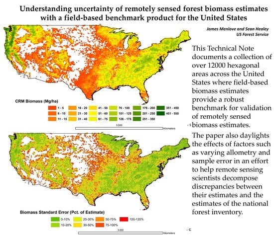
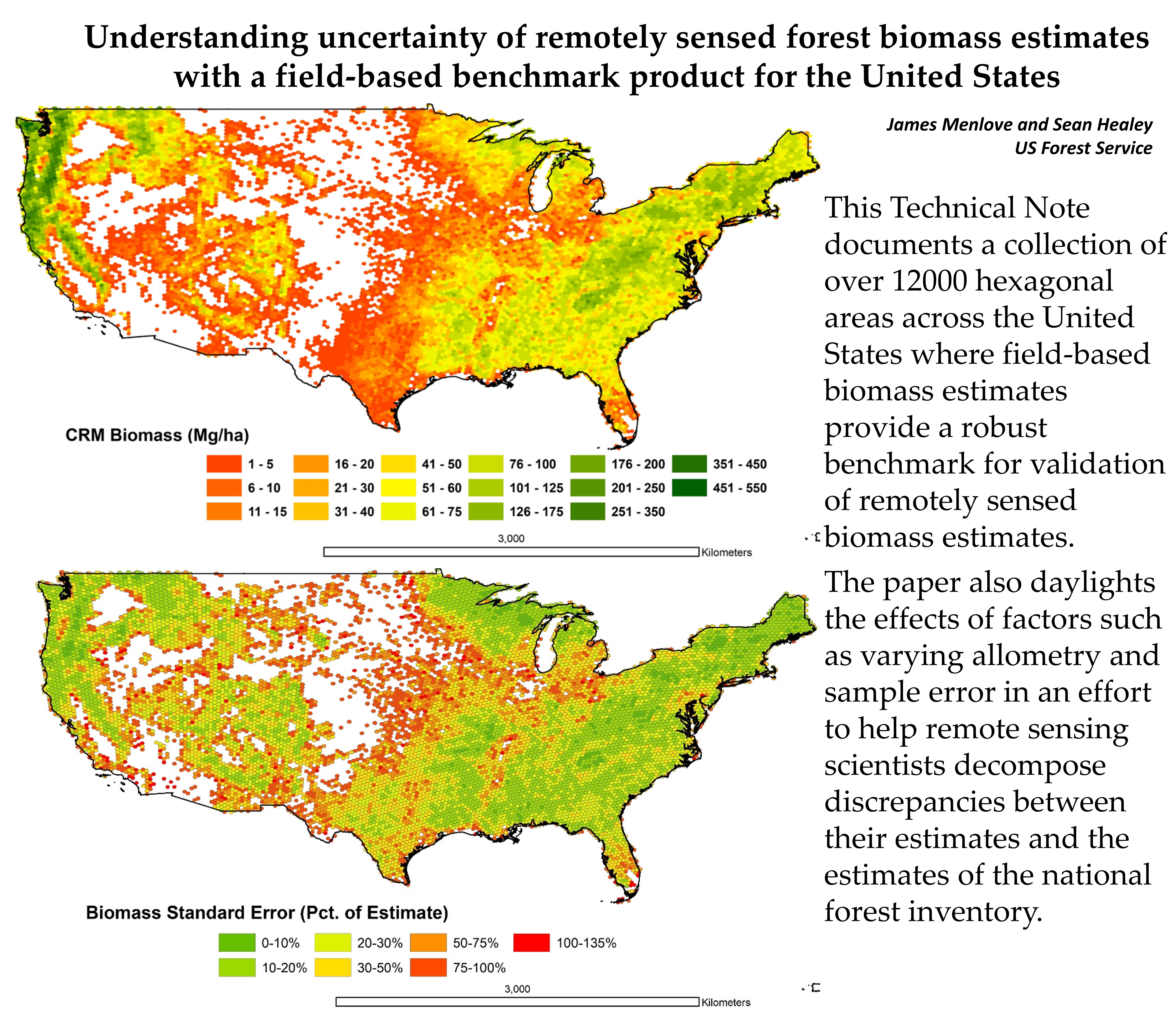
A Comprehensive Forest Biomass Dataset for the USA Allows Customized Validation of Remotely Sensed Biomass Estimates


Abstract
:
1. Introduction
2. Materials and Methods
2.1. Environmental Monitoring and Assessment Program (EMAP) Hexagons
2.2. FIA Measures of Biomass
3. Results
4. Discussion
5. Conclusions
Supplementary Materials
Author Contributions
Funding
Conflicts of Interest
References
- Bonan, G.B. Forests and climate change: Forcings, feedbacks, and the climate benefits of forests. Science (80-) 2008, 320, 1444–1449. [Google Scholar] [CrossRef] [Green Version]
- Schwaab, J.; Bavay, M.; Davin, E.; Hagedorn, F.; Hüsler, F.; Lehning, M.; Schneebeli, M.; Thürig, E.; Bebi, P. Carbon storage versus albedo change: Radiative forcing of forest expansion in temperate mountainous regions of Switzerland. Biogeosciences 2015, 12, 467–487. [Google Scholar] [CrossRef] [Green Version]
- Woodall, C.W.; Coulston, J.W.; Domke, G.M.; Walters, B.F.; Wear, D.N.; Smith, J.E.; Andersen, H.-E.; Clough, B.J.; Cohen, W.B.; Griffith, D.M. The US Forest Carbon Accounting Framework: Stocks and Stock Change, 1990–2016; USDA: Ashville, NC, USA, 2015; Volume 154, pp. 1–49. [Google Scholar]
- Woodall, C.W.; Walters, B.F.; Coulston, J.W.; D’Amato, A.W.; Domke, G.M.; Russell, M.B.; Sowers, P.A. Monitoring Network Confirms Land Use Change is a Substantial Component of the Forest Carbon Sink in the eastern United States. Sci. Rep. 2015, 5, 17028. [Google Scholar] [CrossRef] [Green Version]
- Thom, D.; Rammer, W.; Seidl, R. The impact of future forest dynamics on climate: Interactive effects of changing vegetation and disturbance regimes. Ecol. Monogr. 2017, 87, 665–684. [Google Scholar] [CrossRef] [Green Version]
- Zeng, W.; Tomppo, E.; Healey, S.P.; Gadow, K.V. The national forest inventory in China: History–results–international context. For. Ecosyst. 2015, 2, 23. [Google Scholar] [CrossRef] [Green Version]
- Neuenschwander, A.; Pitts, K. The ATL08 land and vegetation product for the ICESat-2 Mission. Remote Sens. Environ. 2019, 221, 247–259. [Google Scholar] [CrossRef]
- Dubayah, R.; Blair, J.B.; Goetz, S.; Fatoyinbo, L.; Hansen, M.; Healey, S.; Hofton, M.; Hurtt, G.; Kellner, J.; Luthcke, S.; et al. The Global Ecosystem Dynamics Investigation: High-resolution laser ranging of the Earth’s forests and topography. Sci. Remote Sens. 2020, 1, 100002. [Google Scholar] [CrossRef]
- Kimura, T.; Imai, T.; Sakaizawa, D.; Murooka, J.; Mitsuhashi, R. The overview and status of vegetation Lidar mission, MOLI. In Proceedings of the 2017 IEEE International Geoscience and Remote Sensing Symposium (IGARSS), Fort Worth, TX, USA, 23–28 July 2017; pp. 4228–4230. [Google Scholar]
- Quegan, S.; Le Toan, T.; Chave, J.; Dall, J.; Exbrayat, J.-F.; Minh, D.H.T.; Lomas, M.; D’Alessandro, M.M.; Paillou, P.; Papathanassiou, K.; et al. The European Space Agency BIOMASS mission: Measuring forest above-ground biomass from space. Remote Sens. Environ. 2019, 227, 44–60. [Google Scholar] [CrossRef] [Green Version]
- Yu, Y.; Saatchi, S. Sensitivity of L-Band SAR Backscatter to Aboveground Biomass of Global Forests. Remote Sens. 2016, 8, 522. [Google Scholar] [CrossRef] [Green Version]
- Gorelick, N.; Hancher, M.; Dixon, M.; Ilyushchenko, S.; Thau, D.; Moore, R. Google Earth Engine: Planetary-scale geospatial analysis for everyone. Remote Sens. Environ. 2017, 202, 18–27. [Google Scholar] [CrossRef]
- Healey, S.P.; Yang, Z.; Gorelick, N.; Ilyushchenko, S. Highly Local Model Calibration with a New GEDI LiDAR Asset on Google Earth Engine Reduces Landsat Forest Height Signal Saturation. Remote Sens. 2020, 12, 2840. [Google Scholar] [CrossRef]
- Armston, J.; Nickeson, J.; Duncanson, L.; Disney, M.; Camacho, F.; Roman, M. Overview and Status of the CEOS Land Product Validation Subgroup. In Proceedings of the EGU General Assembly Conference Abstracts, Vienna, Austria, 8–13 April 2018; p. 13297. [Google Scholar]
- Duncanson, L.; Neuenschwander, A.; Hancock, S.; Thomas, N.; Fatoyinbo, T.; Simard, M.; Silva, C.A.; Armston, J.; Luthcke, S.B.; Hofton, M.; et al. Biomass estimation from simulated GEDI, ICESat-2 and NISAR across environmental gradients in Sonoma County, California. Remote Sens. Environ. 2020, 242, 111779. [Google Scholar] [CrossRef]
- Bell, D.M.; Gregory, M.J.; Kane, V.; Kane, J.; Kennedy, R.E.; Roberts, H.M.; Yang, Z. Multiscale divergence between Landsat- and lidar-based biomass mapping is related to regional variation in canopy cover and composition. Carbon Balance Manag. 2018, 13, 15. [Google Scholar] [CrossRef] [Green Version]
- Bechtold, W.A.; Patterson, P.L. The Enhanced Forest Inventory and Analysis Program—National Sampling Design and Estimation Procedures; USDA Forest Service Southern Research Station: Ashville, NC, USA, 2005. [Google Scholar]
- Blackard, J.A.; Finco, M.V.; Helmer, E.H.; Holden, G.R.; Hoppus, M.L.; Jacobs, D.M.; Lister, A.J.; Moisen, G.G.; Nelson, M.D.; Riemann, R.; et al. Mapping U.S. forest biomass using nationwide forest inventory data and moderate resolution information. Remote Sens. Environ. 2008, 112, 1658–1677. [Google Scholar] [CrossRef]
- Wilson, B.T.; Knight, J.F.; McRoberts, R.E. Harmonic regression of Landsat time series for modeling attributes from national forest inventory data. ISPRS J. Photogramm. Remote Sens. 2018, 137, 29–46. [Google Scholar] [CrossRef]
- Brown, S.L.; Schroeder, P.E. Spatial patterns of aboveground production and mortality of woody biomass for Eastern U.S. Forests. Ecol. Appl. 1999, 9, 968–980. [Google Scholar] [CrossRef]
- Zhao, F.; Guo, Q.; Kelly, M. Allometric equation choice impacts lidar-based forest biomass estimates: A case study from the Sierra National Forest, CA. Agric. For. Meteorol. 2012, 165, 64–72. [Google Scholar] [CrossRef]
- Vorster, A.G.; Evangelista, P.H.; Stovall, A.E.L.; Ex, S. Variability and uncertainty in forest biomass estimates from the tree to landscape scale: The role of allometric equations. Carbon Balance Manag. 2020, 15, 8. [Google Scholar] [CrossRef]
- Domke, G.M.; Woodall, C.W.; Smith, J.E. Accounting for density reduction and structural loss in standing dead trees: Implications for forest biomass and carbon stock estimates in the United States. Carbon Balance Manag. 2011, 6, 14. [Google Scholar] [CrossRef] [Green Version]
- Healey, S.P.; Menlove, J. The stability of mean wood specific gravity across stand age in US forests despite species turnover. Forests 2019, 10, 114. [Google Scholar] [CrossRef] [Green Version]
- Schnell, S.; Altrell, D.; Ståhl, G.; Kleinn, C. The contribution of trees outside forests to national tree biomass and carbon stocks—A comparative study across three continents. Environ. Monit. Assess. 2014, 187, 4197. [Google Scholar] [CrossRef]
- Huang, W.; Swatantran, A.; Johnson, K.; Duncanson, L.; Tang, H.; O’Neil Dunne, J.; Hurtt, G.; Dubayah, R. Local discrepancies in continental scale biomass maps: A case study over forested and non-forested landscapes in Maryland, USA. Carbon Balance Manag. 2015, 10, 19. [Google Scholar] [CrossRef] [Green Version]
- White, D.; Kimerling, J.A.; Overton, S.W. Cartographic and Geometric Components of a Global Sampling Design for Environmental Monitoring. Cartogr. Geogr. Inf. Syst. 1992, 19, 5–22. [Google Scholar] [CrossRef]
- Woodall, C.W.; Perry, C.H.; Miles, P.D. The relative density of forests in the United States. For. Ecol. Manag. 2006, 226, 368–372. [Google Scholar] [CrossRef]
- Woudenberg, S.W.; Conkling, B.L.; O’Connell, B.M.; LaPoint, E.B.; Turner, J.A.; Waddell, K.L. The Forest Inventory and Analysis Database: Database Description and Users Manual Version 4.0 for Phase 2; RMRS-GTR-2; Forest Service Rocky Mountain Research Station: Fort Collins, CO, USA, 2010. [Google Scholar]
- Pugh, S.A.; Turner, J.A.; Burrill, E.A.; Davide, W. The Forest Inventory and Analysis Database: Population Estimation User Guide; USDA Forest Service: Ashville, NC, USA, 2018. [Google Scholar]
- Moisen, G.G.; McConville, K.S.; Schroeder, T.A.; Healey, S.P.; Finco, M.V.; Frescino, T.S. Estimating Land Use and Land Cover Change in North Central Georgia: Can Remote Sensing Observations Augment Traditional Forest Inventory Data? Forests 2020, 11, 856. [Google Scholar] [CrossRef]
- Jenkins, J.C.; Chojnacky, D.C.; Heath, L.S.; Birdsey, R.A. Comprehensive Database of Diameter-based Biomass Regressions for North American Tree Species; GTR-NE-319; USDA Forest Service, Northeastern Research Station: Newtown Square, PA, USA, 2004. [Google Scholar]
- Woodall, C.W.; Heath, L.S.; Domke, G.M.; Nichols, M.C. Methods and Equations for Estimating Aboveground Volume, Biomass, and Carbon for Trees in the US Forest Inventory; GTR-NRS-88; USDA Forest Service Northern Research Station: Newtown Square, PA, USA, 2011. [Google Scholar]
- Scott, C.T.; Bechtold, W.A.; Reams, G.A.; Smith, W.D.; Westfall, J.A.; Hansen, M.H.; Moisen, G.G. Sample-based estimators used by the forest inventory and analysis national information management system. In General Technical Report SRS-80; US Dept. Ag. For. Service: Ashville, NC, USA, 2005; pp. 53–77. [Google Scholar]
- Chen, Q.; McRoberts, R.E.; Wang, C.; Radtke, P.J. Forest aboveground biomass mapping and estimation across multiple spatial scales using model-based inference. Remote Sens. Environ. 2016, 184, 350–360. [Google Scholar] [CrossRef]
- Patterson, P.L.; Healey, S.P.; Ståhl, G.; Saarela, S.; Holm, S.; Andersen, H.E.; Dubayah, R.O.; Duncanson, L.; Hancock, S.; Armston, J.; et al. Statistical properties of hybrid estimators proposed for GEDI - NASA’s global ecosystem dynamics investigation. Environ. Res. Lett. 2019, 14, 065007. [Google Scholar] [CrossRef]
- Saarela, S.; Holm, S.; Healey, S.P.; Andersen, H.E.; Petersson, H.; Prentius, W.; Patterson, P.L.; Næsset, E.; Gregoire, T.G.; Ståhl, G. Generalized hierarchical model-based estimation for aboveground biomass assessment using GEDI and landsat data. Remote Sens. 2018, 10, 1–27. [Google Scholar] [CrossRef] [Green Version]
- Nelson, R.; Margolis, H.; Montesano, P.; Sun, G.; Cook, B.; Corp, L.; Andersen, H.E.; DeJong, B.; Pellat, F.P.; Fickel, T.; et al. Lidar-based estimates of aboveground biomass in the continental US and Mexico using ground, airborne, and satellite observations. Remote Sens. Environ. 2017, 188, 127–140. [Google Scholar] [CrossRef] [Green Version]
- Healey, S.P.; Patterson, P.L.; Saatchi, S.; Lefsky, M.A.; Lister, A.J.; Freeman, E.A. A sample design for globally consistent biomass estimation using lidar data from the Geoscience Laser Altimeter System (GLAS). Carbon Balance Manag. 2012, 7, 1–9. [Google Scholar] [CrossRef] [Green Version]
- Neeti, N.; Kennedy, R. Comparison of national level biomass maps for conterminous US: Understanding pattern and causes of differences. Carbon Balance Manag. 2016, 11, 19. [Google Scholar] [CrossRef] [Green Version]
- Huang, W.; Dolan, K.; Swatantran, A.; Johnson, K.; Tang, H.; O’Neil-Dunne, J.; Dubayah, R.; Hurtt, G. High-resolution mapping of aboveground biomass for forest carbon monitoring system in the Tri-State region of Maryland, Pennsylvania and Delaware, USA. Environ. Res. Lett. 2019, 14, 95002. [Google Scholar] [CrossRef] [Green Version]
- Domke, G.M.; Woodall, C.W.; Smith, J.E.; Westfall, J.A.; McRoberts, R.E. Consequences of alternative tree-level biomass estimation procedures on U.S. forest carbon stock estimates. For. Ecol. Manag. 2012, 270, 108–116. [Google Scholar] [CrossRef]
- Duncanson, L.; Huang, W.; Johnson, K.; Swatantran, A.; McRoberts, R.E.; Dubayah, R. Implications of allometric model selection for county-level biomass mapping. Carbon Balance Manag. 2017, 12, 18. [Google Scholar] [CrossRef]
- Negrón, J.F.; Cain, B. Mountain Pine Beetle in Colorado: A Story of Changing Forests. J. For. 2019, 117, 144–151. [Google Scholar] [CrossRef] [Green Version]
- Healey, S.P.; Cohen, W.B.; Spies, T.A.; Moeur, M.; Pflugmacher, D.; Whitley, M.G.; Lefsky, M. The relative impact of harvest and fire upon landscape-level dynamics of older forests: Lessons from the Northwest Forest Plan. Ecosystems 2008, 11, 1106–1119. [Google Scholar] [CrossRef] [Green Version]
- Ai, J.; Jia, G.; Epstein, H.E.; Wang, H.; Zhang, A.; Hu, Y. MODIS-Based Estimates of Global Terrestrial Ecosystem Respiration. J. Geophys. Res. Biogeosci. 2018, 123, 326–352. [Google Scholar] [CrossRef]
- Bater, C.W.; Coops, N.C.; Gergel, S.E.; LeMay, V.; Collins, D. Estimation of standing dead tree class distributions in northwest coastal forests using lidar remote sensing. Can. J. For. Res. 2009, 39, 1080–1091. [Google Scholar] [CrossRef]
- Pesonen, A.; Maltamo, M.; Eerikäinen, K.; Packalèn, P. Airborne laser scanning-based prediction of coarse woody debris volumes in a conservation area. For. Ecol. Manag. 2008, 255, 3288–3296. [Google Scholar] [CrossRef]
- Cohen, W.B.; Yang, Z.; Healey, S.P.; Kennedy, R.E.; Gorelick, N. A LandTrendr multispectral ensemble for forest disturbance detection. Remote Sens. Environ. 2018, 205, 131–140. [Google Scholar] [CrossRef]
- Birdsey, R.A.; Dugan, A.J.; Healey, S.P.; Dante-Wood, K.; Zhang, F.; Mo, G.; Chen, J.M.; Hernandez, A.J.; Raymond, C.L.; McCarter, J. Assessment of the Influence of Disturbance, Management Activities, and Environmental Factors on Carbon Stocks of US National Forests; Generatl, T., Ed.; USDA Forest Service Rocky Mountain Research Station: Fort Collins, CO, USA, 2019. [Google Scholar]


| EMAP_HEX | FIADB EMAP hexagon identifier. The same as USHEXES_ID in the original EMAP GIS layer. |
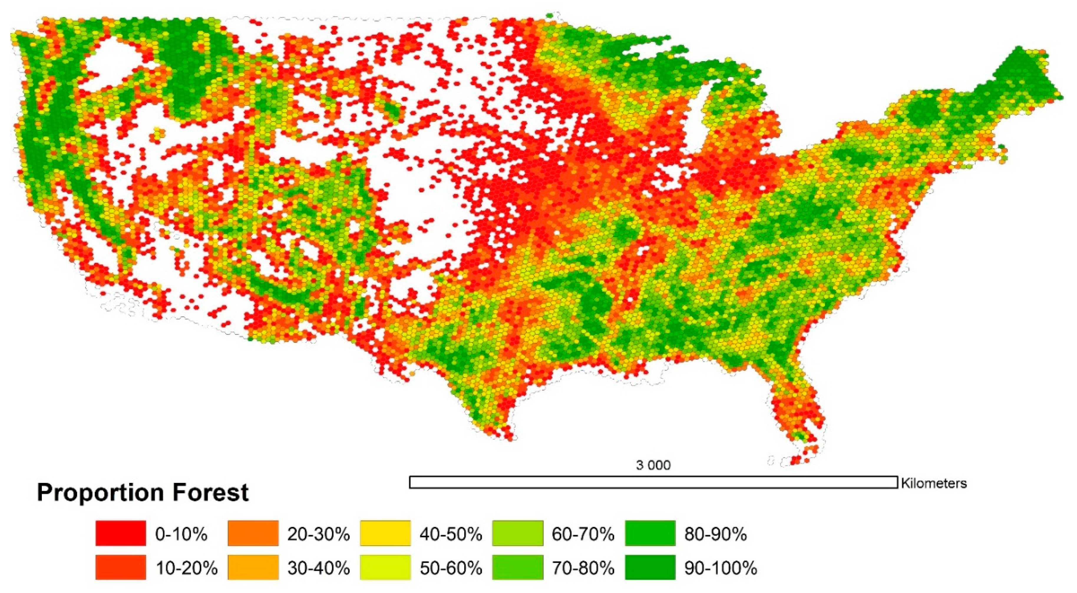
| PROP_FOREST | Estimate of proportion of the area that is forest land. Ratio estimate of forest land area over sampled area. Unitless. |
| SE_PROP_FOREST_PCT | Sampling error of estimate of the forest land proportion, as a percent of the estimate. |
| CRM_LIVE | Estimate of aboveground biomass of live trees (≥2.54 cm diameter) on forest land per hectare of sampled area, using FIA component ratio method (CRM). Megagrams per hectare. |
| SE_CRM_LIVE_PCT | Sampling error of CRM live biomass per hectare estimate, as a percent of the estimate. |
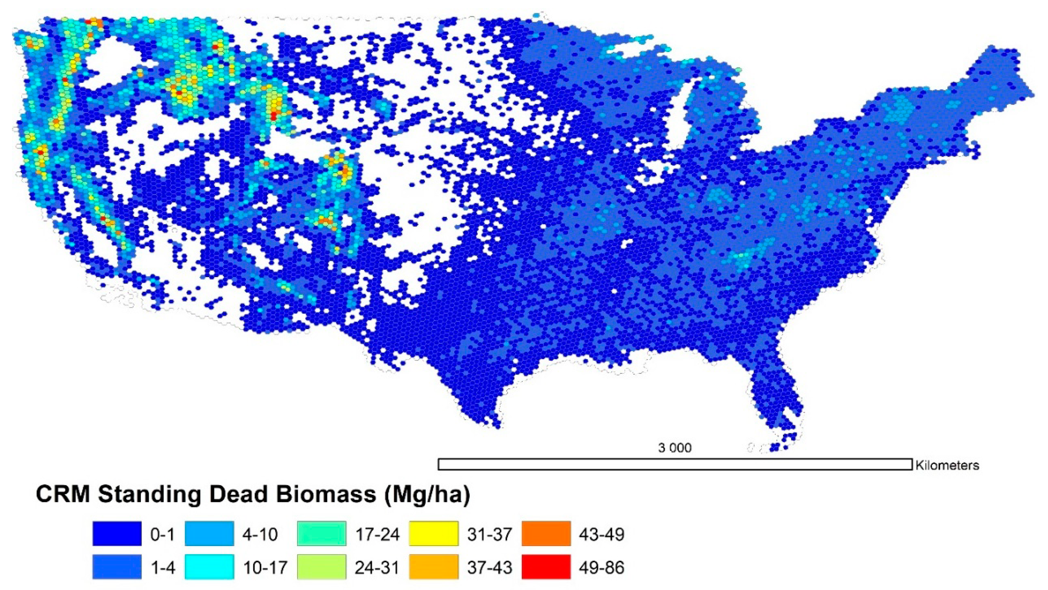
| CRM_STND_DEAD | Estimate of aboveground biomass of standing dead trees (≥12.7 cm diameter) on forest land per hectare of sampled area, using FIA component ratio method (CRM). Megagrams per hectare. |
| SE_CRM_STND_DEAD_PCT | Sampling error of CRM standing dead biomass per hectare estimate, as a percent of the estimate. |
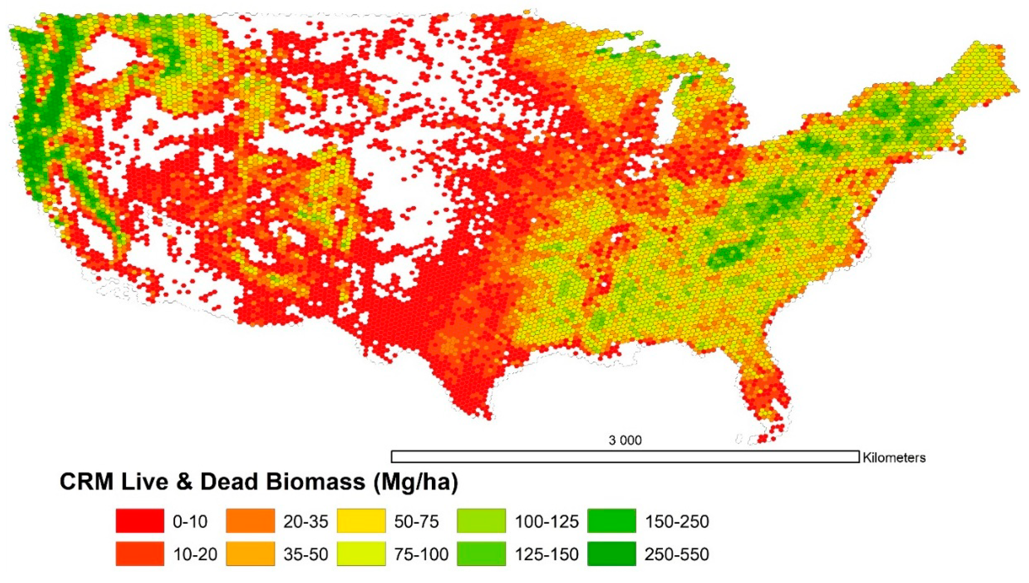
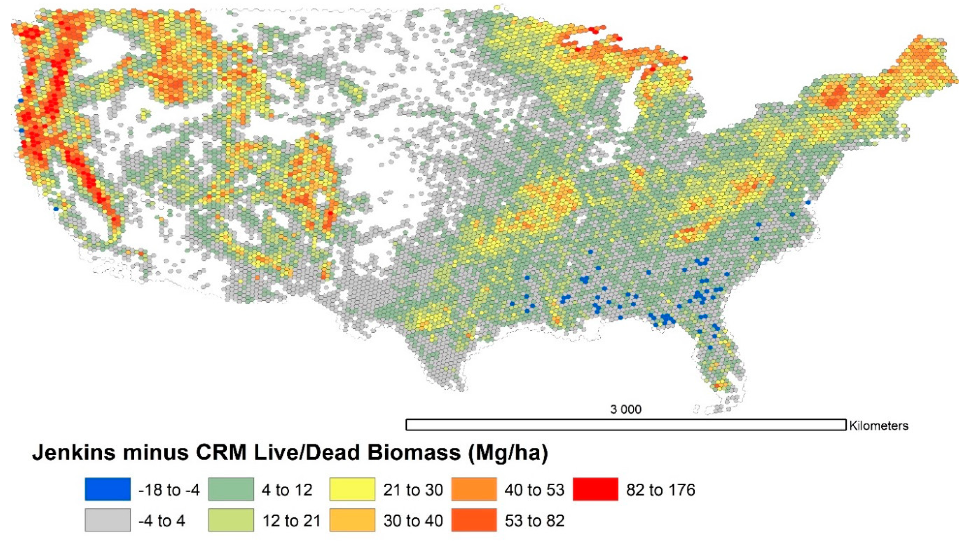
| CRM_LIVE_DEAD | Estimate of aboveground biomass of live trees (≥2.54 cm diameter) plus standing dead trees (≥5 inches diameter) on forest land per hectare of sampled area, using FIA component ratio method (CRM). Megagrams per hectare. |
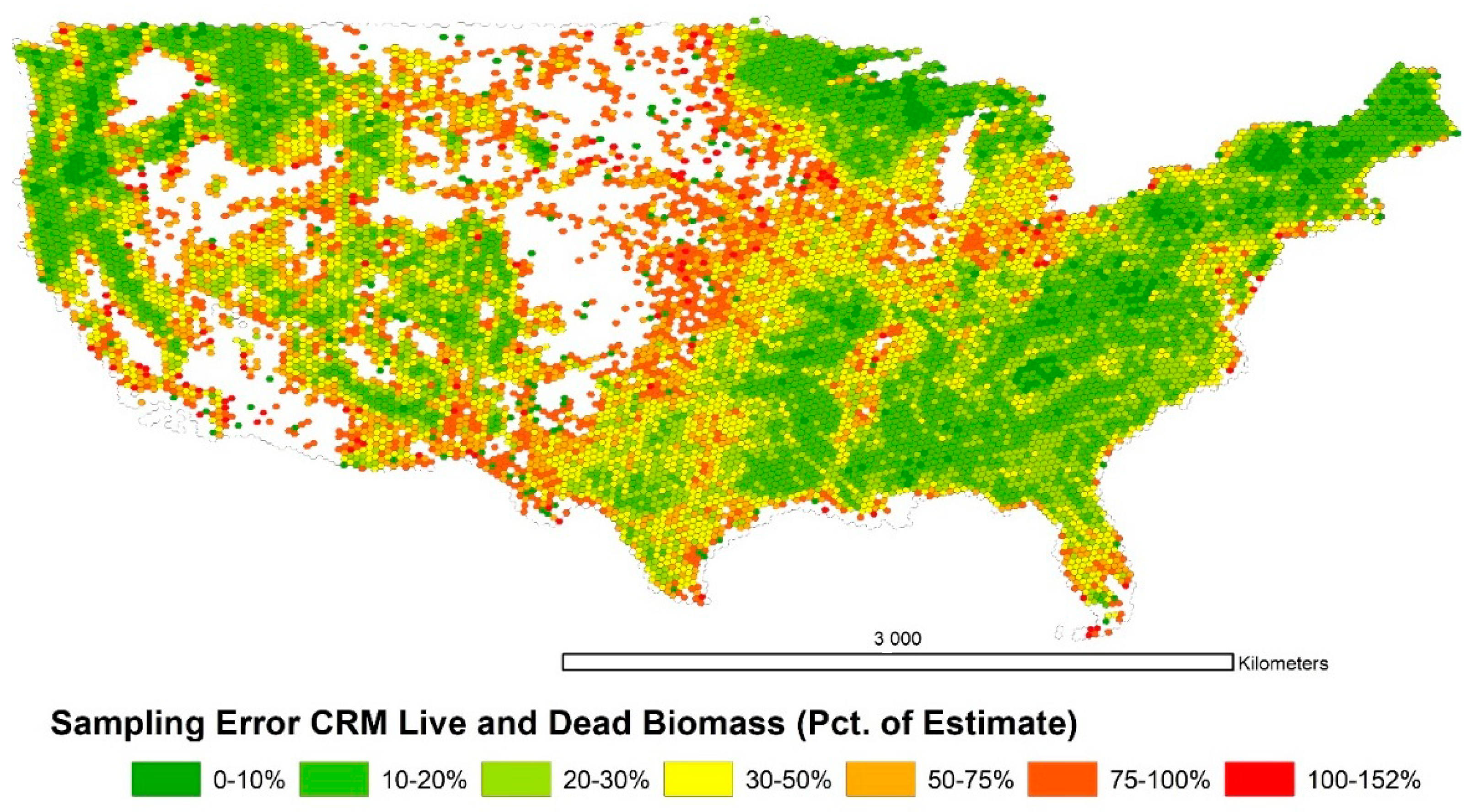
| SE_CRM_LIVE_DEAD_PCT | Sampling error of CRM live plus standing dead biomass per hectare estimate, as a percent of the estimate. |
| DRYBIOT_LIVE | Estimate of aboveground biomass of live trees (≥2.54 cm diameter) on forest land per hectare of sampled area, using retired FIA regional methods. Megagrams per hectare. |
| SE_DRYBIOT_LIVE_PCT | Sampling error of regional method live biomass per hectare estimate, as a percent of the estimate. |
| DRYBIOT_STND_DEAD | Estimate of aboveground biomass of standing dead trees (≥12.7 cm diameter) on forest land per hectare of sampled area, using retired FIA regional methods. Megagrams per hectare. |
| SE_DRYBIOT_STND_DEAD_PCT | Sampling error of regional method standing dead biomass per hectare estimate, as a percent of the estimate. |
| DRYBIOT_LIVE_DEAD | Estimate of aboveground biomass of live trees (≥2.54 cm diameter) plus standing dead trees (≥5 inches diameter) on forest land per hectare of sampled area, using retired FIA regional methods. Megagrams per hectare. |
| SE_DRYBIOT_LIVE_DEAD_PCT | Sampling error of regional method live plus standing dead biomass per hectare estimate, as a percent of the estimate. |
| JENK_LIVE | Estimate of aboveground biomass of live trees (≥2.54 cm diameter) on forest land per hectare of sampled area, using Jenkins equation. Megagrams per hectare. |
| SE_JENK_LIVE_PCT | Sampling error of Jenkins live biomass per hectare estimate, as a percent of the estimate. |
| JENK_STND_DEAD | Estimate of aboveground biomass of standing dead trees (≥12.7 cm diameter) on forest land per hectare of sampled area, using Jenkins equation. Megagrams per hectare. |
| SE_JENK_STND_DEAD_PCT | Sampling error of Jenkins standing dead biomass per hectare estimate, as a percent of the estimate. |
| JENK_LIVE_DEAD | Estimate of aboveground biomass of live trees (≥2.54 cm diameter) plus standing dead trees (≥12.7 cm diameter) on forest land per hectare of sampled area, using Jenkins equation. Megagrams per hectare. |
| SE_JENK_LIVE_DEAD_PCT | Sampling error of Jenkins live plus standing dead biomass per hectare estimate, as a percent of the estimate. |
| EST_SAMPLED_HA | Estimate of sampled hectares in the hexagon. |
| SAMPLED_PLOTS | Number of sampled plots in the hexagon. |
| NON_SAMPLED_PLOTS | Number of non-sampled plots in the hexagon. |
Publisher’s Note: MDPI stays neutral with regard to jurisdictional claims in published maps and institutional affiliations. |
© 2020 by the authors. Licensee MDPI, Basel, Switzerland. This article is an open access article distributed under the terms and conditions of the Creative Commons Attribution (CC BY) license (http://creativecommons.org/licenses/by/4.0/).
Share and Cite
Menlove, J.; Healey, S.P. A Comprehensive Forest Biomass Dataset for the USA Allows Customized Validation of Remotely Sensed Biomass Estimates. Remote Sens. 2020, 12, 4141. https://doi.org/10.3390/rs12244141
Menlove J, Healey SP. A Comprehensive Forest Biomass Dataset for the USA Allows Customized Validation of Remotely Sensed Biomass Estimates. Remote Sensing. 2020; 12(24):4141. https://doi.org/10.3390/rs12244141
Chicago/Turabian StyleMenlove, James, and Sean P. Healey. 2020. "A Comprehensive Forest Biomass Dataset for the USA Allows Customized Validation of Remotely Sensed Biomass Estimates" Remote Sensing 12, no. 24: 4141. https://doi.org/10.3390/rs12244141