Air Pollution Prediction with Multi-Modal Data and Deep Neural Networks

Abstract

Air pollution is becoming a rising and serious environmental problem, especially in urban areas affected by an increasing migration rate. The large availability of sensor data enables the adoption of analytical tools to provide decision support capabilities. Employing sensors facilitates air pollution monitoring, but the lack of predictive capability limits such systems’ potential in practical scenarios. On the other hand, forecasting methods offer the opportunity to predict the future pollution in specific areas, potentially suggesting useful preventive measures. To date, many works tackled the problem of air pollution forecasting, most of which are based on sequence models. These models are trained with raw pollution data and are subsequently utilized to make predictions. This paper proposes a novel approach evaluating four different architectures that utilize camera images to estimate the air pollution in those areas. These images are further enhanced with weather data to boost the classification accuracy. The proposed approach exploits generative adversarial networks combined with data augmentation techniques to mitigate the class imbalance problem. The experiments show that the proposed method achieves robust accuracy of up to 0.88, which is comparable to sequence models and conventional models that utilize air pollution data. This is a remarkable result considering that the historic air pollution data is directly related to the output—future air pollution data, whereas the proposed architecture uses camera images to recognize the air pollution—which is an inherently much more difficult problem.

1. Introduction

Air pollution represents a major issue in modern society, especially with the increasing migrations into urban areas. As a result, many efforts are directed towards building successful monitoring systems, including sensors and cameras, which collect data continuously.

According to the authors of [1], 70% of the world’s population will live in urban centers by 2050, which means that efficient solutions are required to monitor and predict air pollution. As stated in [2], North America and Australia are the least polluted regions, followed by Central Europe, while India and Asia exhibit the highest air pollution. Even if not much information is available for South America and Africa, the limited available data suggest that air pollution levels are high in these areas as well. The main cause of death for children under the age of 15 is air pollution, with 600,000 deaths every year, according to a report done by the World Health Organization [3]. Based on research done in [4], air pollution contributes towards 7 million deaths a year, and 92% of the world’s population is breathing toxic air. In less developed countries, 98% of children under five years old breathe toxic air. In financial terms, premature deaths due to air pollution cost about $5 trillion in welfare losses worldwide [5].

In recent years, the Internet of Things (IoT) paradigm has emerged, empowering objects of everyday life with microcontrollers, transceivers for digital communication, and a suitable protocol stack, which enables them to communicate with one another and with the users, becoming an integral part of the Internet [6]. Thanks to this addition, devices such as home appliances, surveillance cameras, sensors, and vehicles can generate enormous amounts of various data that can be subsequently analyzed and used to develop new applications. Recent advances in IoT technologies have allowed people to develop efficient systems consisting of multiple sensors connected wirelessly, either by Bluetooth or WiFi for nearby regions, or mobile networks and satellite for remote regions to monitor the different air pollutants in different regions. These volumes of diverse data might need parallelization using big data and cloud computing technologies to be able to analyze emerging patterns [7], and facilitate near real-time monitoring. Monitoring systems allow us to collect quality data, which can then be used to extract deeper knowledge about pollution [8,9].

Air pollution forecasting systems enable us to predict the Air Quality Index (AQI), the value of each pollutant, such as particle matter (PM) or carbon dioxide concentration (i.e., PM2.5, PM10, CO₂, etc.), and recognize high-pollution areas. Predictive air pollution systems can help governments employ smarter solutions and preventive measures to address air quality problems. Although many solutions and models for predicting air pollution have been proposed in the literature, they generally can be classified into two categories. The first category is models for tracking the generation, dispersion, and transmission process of pollutants. Numerical simulations generate the predictive results of these models. The second category includes statistical learning models, machine learning, and deep learning models. These models attempt to extract patterns directly from the input data, learning from the data distribution [10].

Recent advances in deep learning techniques and the high amount of data available have inspired many authors to develop and implement different prediction models, as discussed in more details in the related work section [10,11,12,13,14,15,16,17]. Nevertheless, the results achieved in the literature are not conclusive. Therefore, air pollution prediction remains an important and active area of research. In particular, the exploitation of images for air pollution prediction task remains an unexplored area and require more attention.

High-quality predictions in this domain are important due to their impact on the everyday life of citizens. In particular, knowing in advance about high-pollution events can result in initiatives such as traffic reduction policies, closure of public venues including schools, as well as recommendations to limit exposure for sensitive people. In turn, high-quality predictions require proper detection techniques that are tailored to the problem at hand and can address inherent challenges such as the ability to handle class imbalance and exploit multimodal data.

This paper proposes a novel approach based on convolutional neural networks (CNNs) that exploit camera images for predicting air pollution. The motivation to use camera images instead of air pollution sensors is because of the immense IoT infrastructure consisting of security and traffic light cameras, even in developing countries where air pollution sensors are sparse. An air pollution estimation approach based on cameras can facilitate generating a real-time heat-map of air pollution and tracking pollution sources.

We propose and evaluate four architectures for classifying images and show that using generative approaches enhanced with standard data augmentation methods for handling imbalanced datasets leads to better performance than state-of-the-art methods. Most air pollution methods rely on raw or processed air pollution data, such as historic sensory measurements of pollutants [10,11,12,13,14,15,16,17]. Differently than existing approaches in the literature, the novelty of our work stands in the exploitation of generative adversarial neural networks combined with data augmentation techniques, as well as the adoption of multi-modal data consisting of sensor measurements and camera images. Combining these aspects allows us to tackle challenges related to the predictive task, including the presence of class imbalanced data, the partial and potentially noisy information deriving from a single source of data, and the exposure to adversarial attacks. As a result, the resulting predictive model appears more robust and accurate than existing solutions in the literature.

The remainder of this paper is organized as follows. Section 2 presents related work for handling the problem of air pollution prediction. The architecture of the proposed models and the evaluated data augmentation techniques are explained in Section 3. In Section 4, we provide the evaluation results of our models and in Section 5 we discuss them. Finally, Section 6 concludes the paper and proposes promising future work directions.

2. Related Work

In Section 2.1 we first cover deep learning approaches for classification in remote sensing context. Then, in Section 2.2 and Section 2.3 we describe the recent approaches for mitigating the class imbalance challenge in image data and more specifically in remote sensing problems. Furthermore, we highlight how the proposed method differs from the existing approaches. Finally, in Section 2.4 we review the recent approaches for air pollution prediction.

2.1. Deep Learning Classification in Remote Sensing

Transfer learning appears successful in classification tasks involving remote sensing data. One such example is presented in [18], which investigates a simple and effective transfer learning strategy that uses unsupervised pre-training step without label information. This capability is confirmed in other studies as in [19], which shows how CNNs perform when applied under operational emergency conditions, with unseen data and time constraints, in the context of automated building damage assessment. Similarly, transfer learning has been successfully adopted in different studies focusing on aerial scene classification [20,21], where fine-tuning and adaptive learning rates are proposed. The fine-tuned neural networks are subsequently used for feature extraction and remote sensing image classification with a Support Vector Machine (SVM) model with linear and Radial Basis Function (RBF) kernels. However, approaches based on transfer learning, which leverage pre-trained deep neural networks to perform classification of new datasets, appear unreliable in the presence of class imbalanced datasets. This behavior was shown in [22], where the goal was to detect invasive blueberry species in aerial images of wetlands. The authors showed that their pre-trained network achieved a general high classification accuracy while largely ignoring the blueberry class, thus failing in the study’s main goal. For this reason, custom approaches to mitigate class imbalanced data are required.

2.2. Imbalanced Data in Remote Sensing

A sampling-based approach was proposed in [23], where a case-control mechanism was adopted to select a large fraction of pixels with the outcome of interest. This approach has shown considerably better inference and prediction than random sampling. A different data augmentation approach was used in [24], where the authors includes depth of sampling as a covariate to perform a national scale 3D mapping of soil pH. Another approach based on hybrid data balancing called Partial Random Over-Sampling and Random Under-Sampling was investigated in [25]. This study applied it successfully in an unbalanced dataset for the classification of Google Earth images in mountainous regions. An ensemble-based method to handle imbalanced data in the context of land cover mapping is proposed in [26]. In this study, the authors integrate random under-sampling of majority classes and an ensemble of Support Vector Machines. A multi-scale feature fusion approach was presented in [27], where the authors proposed a fully convolutional neural network called DeepLab V3+, which loss function gives increased weights to imbalanced samples. On the same thread of approaches, Ref. [28] proposed a dual-attention capsule U-Net (DA-CapsUNet) for road region extraction, which combines the properties of capsule representations and attention mechanisms intending to increase the robustness of the model. Feature extraction approaches are proposed in [29] where the authors extract ship features of different levels and propose fusing fine-grained features from shallow layers with semantic features from deep layers to detect ship targets with different sizes.

2.3. Imbalanced Data in Images

Image classification datasets are often imbalanced, which negatively affects the accuracy of most classifiers. To mitigate this problem, many strategies have been proposed in the research community.

One of the most frequently used technique in the past was random oversampling and undersampling [30]. With these approaches, in every training epoch, images from the minority class are taken more frequently, or images from the majority class are taken with less frequency.

However, in recent years, more advanced techniques, such as Generative Adversarial Networks (GAN), are gaining popularity. One such approach is explained in [31], where GAN is used to balance the imbalanced image dataset. The model is first trained with the majority and minority class. This allows the model to learn useful features from the majority class. In a subsequent phase, these features and then used to generate images for minority classes.

Another interesting approach is explained in [32], where the authors exploit using GAN architecture for Medical Image Augmentation in Liver Lesion Classification. They show that by using the GAN architecture, they significantly improve the classifier’s performances. A similar approach for chest X-ray generation is explained in [33], where the authors employ the GAN architecture to generate new images. They explain that obtaining medical annotated images is difficult and show that the classifier’s performance significantly benefits from the generative strategy. Another approach showing the advantages of the GAN network is explained in [34], where the GAN architecture is used in two brain segmentation tasks. The difference between our approach and the previously explained approaches is that we use only the minority class to train the GAN architecture and then use this trained GAN architecture to generate new images for the minority class, thus balancing the dataset.

2.4. Air Pollution Prediction

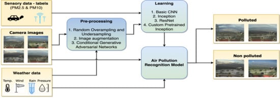
Recently, extensive research was devoted to air pollution prediction considering traditional and deep learning approaches. While many different models have been proposed, they mainly exploit pollution measurements collected from sensors at specific times and locations. The considered pollutants are usually the particulate matter (i.e., PM2.5 and PM10) and gaseous species (i.e., NO₂, CO, O₃, and SO₂). Meteorological data such as humidity, temperature, wind speed, and rainfall are also integrated, with some approaches even incorporating weather forecast data, as explained in [11,35].

The data preprocessing pipeline mainly consists of a feature extraction step, where the most common approaches are Principal Component Analysis (PCA), cluster analysis, factor analysis, and discriminant analysis. Data fusion is performed by leveraging simple techniques, such as matching and aggregation by time and location, as well as interpolation. The modeling and the preprocessing stages are usually executed separately, as explained in [10,14,15,35,36,37]. Still, some approaches incorporate this stage of the feature analysis or interpolation directly into the model architecture [11,13].

A large number of methods available in the literature can be separated into two different categories. The first category of methods are predicting the level of pollutants (such as PM2.5, PM10, NO₂, etc.), such as [9,10,12,15,36,38]. The second category consists of methods predicting the pollution level in the form of Air Quality Index (AQI) or Air Pollution Index, such as [11,13,14,35]. The key difference between the two categories of methods stands in the labeling of the pollutant data. While methods in the first category of methods do not require labeling since the purpose is to predict the actual pollutant values, the second category of methods require labeling fine-grained data so it can be used to train supervised classification algorithms. Recently, both types of models are based on deep neural networks [11,12,13] or improvements of the classical fully-connected neural networks such as Recurrent Neural Networks [10] (RNN) and Long Short-Term Memory (LSTM) networks, as special types of RNN [14]. In addition, some approaches exploit autoencoder models [15,39], sequence-to-sequence models [17], neural networks that combine linear predictors as ensembles [35], Bayesian networks and multi-label classifiers [36]. Another interesting approach is explained in [40], where an attention-based model is adopted. This approach’s attention mechanism is applied only on the wind measurements to obtain an encoded value used as a data augmentation technique in the main model. The [40,41] attention-based approaches are applied to all available weather and pollution information. Some approaches combine the ideas of convolutional neural networks (CNN) to further augment the performance of pollution prediction achieved by the RNN models [42,43,44]. The approaches use different evaluation methods, but they generally adopt standard evaluation measures for regression, such as Root Mean Square Error (RMSE), Mean Absolute Error (MAE), Mean Absolute Percentage Error (MAPE), Mean Prediction Error (MPE), or Relative Prediction Error (RPE).

Although many deep learning approaches for air pollution prediction have been proposed in the literature, most of them are based on using sequential pollution data coming from sensors to make predictions. On the contrary, air pollution prediction approaches that leverage camera images and CNNs are quite rare. To the best of our knowledge, only two studies investigated this direction. The approach in [45] exploits satellite images and a deep-learning model based on a convolutional neural network architecture to create pollution maps. Similarly to it, our models utilize deep learning approaches but are trained on camera images instead of satellite images. Another approach is explained in [46], where smartphone images are used to make a pollution estimation. The training is based only on 1575 images, and the performance evaluation is with a synthetic dataset. Unlike this approach, ours considers 178,992 images in the training and evaluation process.

3. Methods

This paper proposes a novel approach for air pollution prediction, leveraging the combination of weather data and camera images, evaluating four different architectures. Namely, the input is primarily based on cameras taken from a static camera placed at the Vodno mountain near Skopje, North Macedonia. Next, we use the meteorological data taken from the nearest meteorological station. The output is the predicted Air Quality Index, which is validated based on the nearest PM2.5 sensor measurements. Note that the PM2.5 is used to generate labels for the data to facilitate supervised learning and not as an input itself. The location of all sensors is shown in Figure 1. The workflow of the proposed methodology is shown in Figure 2.

To the best of our knowledge, this is the first study that proposes adopting these two data sources. Moreover, we employ transfer learning in two of the four evaluated architectures, leveraging pre-trained models that are fine-tuned for air pollution prediction. The purpose of transfer learning is to leverage the general knowledge of pre-trained networks, which implies the ability to identify low-level features (such as vertical and horizontal lines), and to train the network further using the target dataset to focus on task-specific features [20,47].

The remainder of this section is structured as follows. First, Section 3.1 describes the four evaluated architectures. The architecture based on a convolutional neural network model is explained in Section 3.1.1. The architecture of the Residual neural network is explained in Section 3.1.2. The architecture of the basic Inception network, as well as our extended Inception network, are explained in Section 3.1.3. Finally, the custom inception-based model is described in Section 3.1.4.

The second part of this section, Section 3.2, describes the different data pre-processing techniques employed in the different architectures.

3.1. Architectures of the Predictive Models

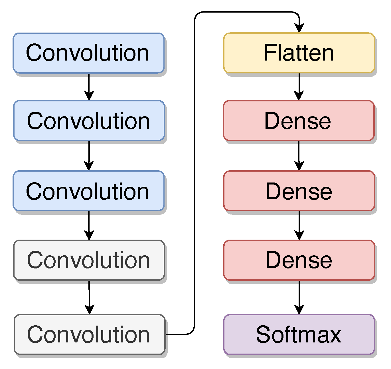
3.1.1. Basic Convolutional Neural Network Model

The main element of the basic convolutional neural network model is the convolution block, which is shown in Figure 3. This block consists of three layers: two convolutional layers and one max pooling layer. These blocks enable the model to learn the low-level features in the images while allowing the upper layers to activate on higher-level features responsible for successful predictions. A convolution layer is a simple application of a filter to an input that results in an activation. Repeated application of the same filter to an input results in a map of activations called feature map, indicating the locations and strength of a detected feature in the input. Consequently, the resulting architecture is shown in Figure 4.

Pooling layers provide an approach for downsampling feature maps by summarizing features in patches of the feature map. Two common pooling methods are average pooling and max pooling, which summarize the average presence of a feature and the most activated presence of a feature, respectively. The flatten layer is also commonly used, which receives the multidimensional input from the convolution layers and flattens it to a one-dimensional input. Likewise, dense layers (fully connected layers) are regularly used to predict the image class based on one-dimensional input. Although this model is much simpler and shallower than the other models, it still provides significant classification capability, as shown in Section 4.

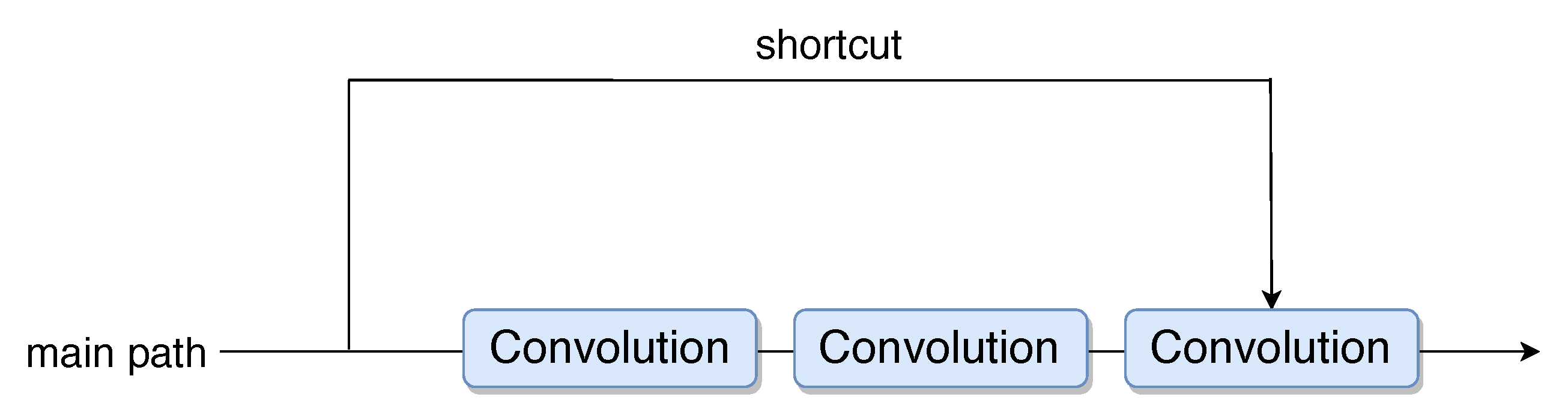
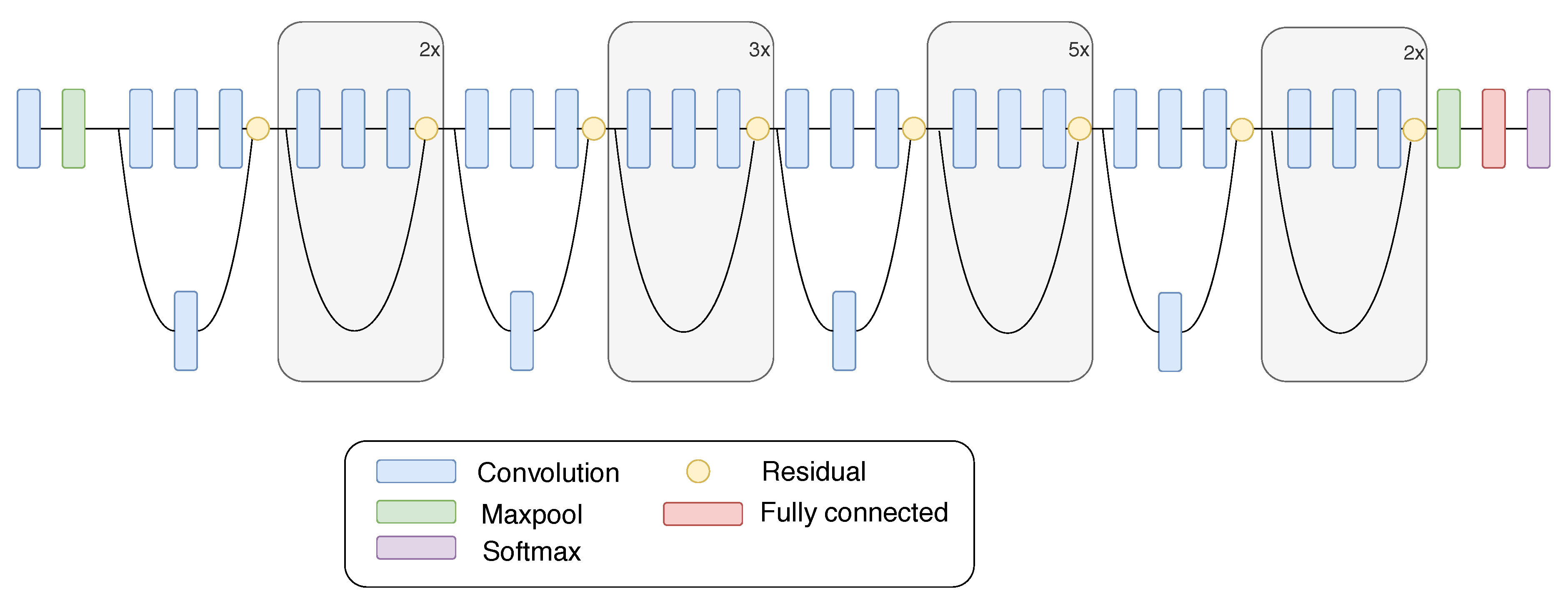
3.1.2. Residual Network Model

The main benefit of a very deep network is that it can represent very complex functions. It can also learn features at many different abstraction levels, from edges (at the shallower layers, closer to the input) to very complex features (at the deeper layers, closer to the output). However, very deep neural networks are difficult to train because of the problem of vanishing gradient [48]. The vanishing gradient problem occurs when the gradient is back-propagated to earlier layers, and the repeated multiplication operations make the gradient infinitely small. As a result, as the network becomes deeper, its performance saturates or even degrades rapidly. This problem inspired the residual network (ResNet) [49], which allows robust deep convolutional neural networks to be built. The main idea of the ResNet model is the residual blocks, whose architecture is shown in Figure 5. The residual block provides two paths for the input: the main path and the shortcut (or more commonly known as skip-path). The main path provides the normal flow as with any convolutional neural network. Still, the shortcut skips N convolution layers (in our approach $N=2$) and provides its input to the following convolution layer. The authors in [49] argue that stacking layers should not degrade the network performance because one could simply stack identity mappings (layers that learn the identity mapping which ultimately does not make any change) upon the current network, and the resulting architecture would perform equally. This indicates that the deeper model should not produce a training error higher than its shallower counterparts. They hypothesize that letting the stacked layers fit a residual mapping is easier than letting them directly fit the desired underlying mapping. The residual block explicitly allows the model to perform this task.

The basic residual block is also known as the identity block. This block corresponds to the case where the input activation has the same dimension as the output activation. Apart from this block, there is another block called the convolutional block. The architecture of this block is shown in Figure 6. In this block, the input and output dimensions do not match. The difference between this block and the identity block is that there is a convolutional layer in the shortcut path to match the dimensions.

The complete architecture of the ResNet model is shown in Figure 7. We can see that the model is built using multiple convolutional and identity blocks. It also contains convolution and max pooling layers at the beginning of the model, as well as flatten and dense layers at the end to make the final prediction. We show in Section 4 that by using this model, we obtain better results, which can be explained by the fact that we can use much deeper networks that can learn complex features and are not affected by the problem of vanishing gradient.

3.1.3. Inception Model

The Inception architecture [50] started as a case study for assessing the hypothetical output of a sophisticated network topology construction algorithm. This algorithm tries to approximate a sparse structure for vision networks and covering the hypothesized outcome by dense, readily available components. With small modifications, it has proven to be quite useful in the problems of localization and object detection as described in [51,52,53].

The main element of this model is the inception block, which instead of choosing the size of the filter such as a $1\times 1$, $3\times 3$, or $5\times 5$ filter, or whether a pooling layer should be present, allows combining all these layers to operate on the same level, resulting in a more complex network architecture, but that ultimately provides better performance. The architecture of the inception block is shown in Figure 8. To mitigate the computational complexity of the deep neural networks, an effective solution is to limit the number of input channels by adding an extra $1\times 1$ convolution before the $3\times 3$ and $5\times 5$ convolutions, as used in [50]. Although adding an extra operation may seem counterintuitive, $1\times 1$ convolutions are far cheaper than $5\times 5$ convolutions due to the reduced number of input channels.

Another part worth mentioning here is that after all convolutional layers have been executed, the concatenation is done per channel (filter). The Inception model’s complete architecture is shown in Figure 9, which ultimately combines the inception blocks with standard layers to create a very deep neural network.

3.1.4. Custom Pretrained Inception

The custom pre-trained inception model leverages the architecture of the Inception model, as explained in Section 3.1.3, while extending it to improve performances further. To have a model that has already learned low-level features such as horizontal and vertical lines, we used the InceptionV3 pre-trained model offered by Keras (https://keras.io/api/applications/inceptionv3/). Apart from using the Inception architecture, we extended it by adding a new sub-model path. This sub-model path takes as input weather data, which goes through three fully connected layers. The weather data taken into consideration for this model are: weather description, precipitation, humidity, and visibility. The weather data are concatenated with the output of the inception model in the last fully connected layer, which then goes to a softmax layer that outputs the predicted class. Figure 10 shows the custom pretrained inception architecture.

3.2. Data Preprocessing

Generally, high air pollution takes place in specific periods of the year, causing a high-class imbalance between the number of data instances available for different levels of air pollutions. Skopje, North Macedonia is not an exception, and the high-class imbalance poses a challenge for any predictive task. Our dataset contains 167,348 images of Skopje’s central area, taken from a camera placed on Vodno. Even though Skopje in the last few years has been in the top 10 most polluted cities in the world, the dataset is highly imbalanced, with about 120,000 images having low air pollution (the non-polluted class), causing a skew in the class distribution. This phenomenon can be explained by the fact that Skopje is highly polluted, mainly in winter and dry days. Consequently, training our model using this type of dataset would ultimately lead the model biased to the non-polluted images. It would lead to over-fitting on the validation and testing set. Imbalanced datasets cause very impactful bottlenecks in CNN networks and need to be addressed. For this reason, we exploit random oversampling and undersampling as well as image augmentation, as explained in the following subsections.

3.2.1. Random Oversampling and Undersampling

We used two different strategies for tackling the class imbalance issue. The first technique is random oversampling and undersampling, as explained in [54]. This technique allows obtaining a balanced dataset by randomly taking multiple copies of minority class images or randomly skipping a portion of the majority class images. These techniques did not prove useful in our problem and did not resolve the imbalance issue, as shown in Section 4.

3.2.2. Image Augmentation

Standard image processing augmentation techniques were applied recurring to the Keras library. Generating new and realistic images with operations such as image flipping and rotation, as well as zooming by small factors, has a big potential in improving the performances of the network. These techniques were applied after both approaches for class balancing described in the following subsections.

3.2.3. Conditional Generative Adversarial Networks (CGAN)

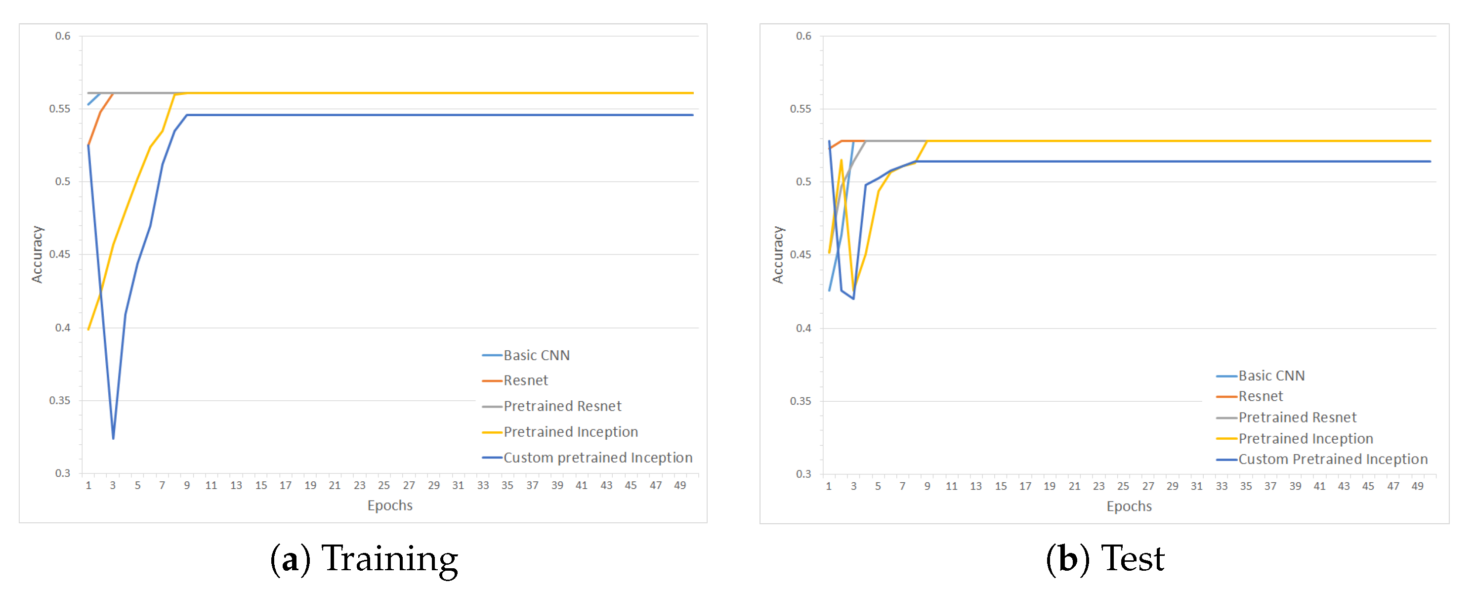
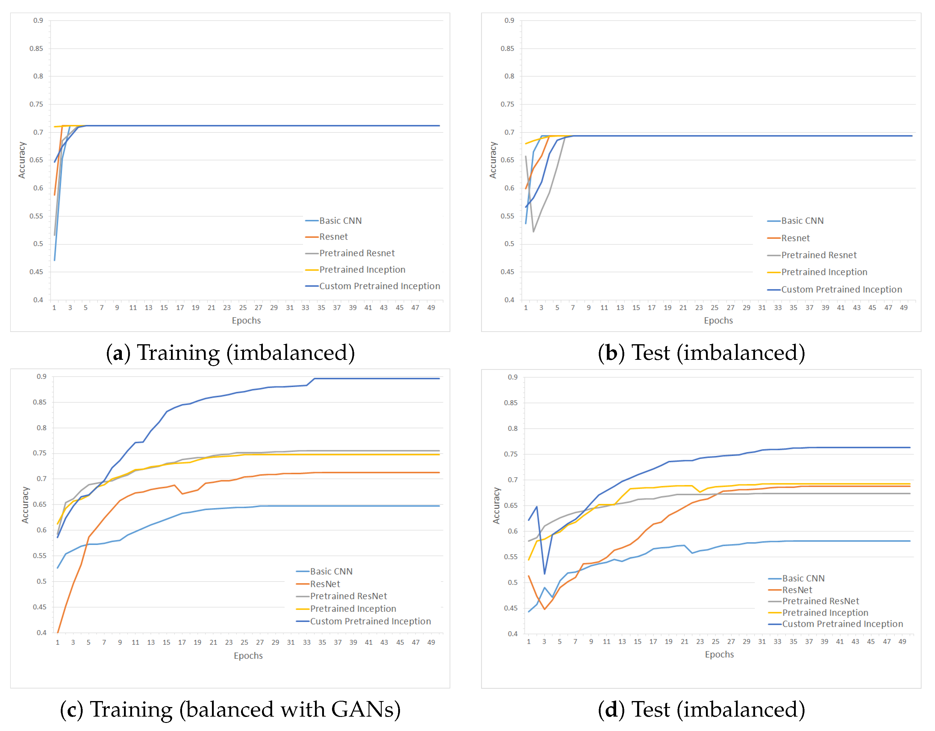
Conditional Generative Adversarial Networks (CGAN) [55] allows us to augment the dataset using generative models. We trained these models to learn how to generate new images based on previously seen images. Specifically, we trained a CGAN model using the minority class’s images in the training set and applied it to generate new images for the same class, mitigating the class imbalance issue. The idea of the CGAN is to augment the dataset and provide us with a training dataset where 50% of the images are from the first class, and the remaining are of the second class. The CGAN is not used in the testing dataset because we want to test our models on the camera’s raw images. After the CGAN is applied and the dataset has been balanced; simple augmentation methods such as flipping images, rotating, and zooming by small factors are applied to the dataset. This additionally improves the performances of our models and provides us with a broader dataset. We show the evaluation of these techniques in Section 4.

4. Results

4.1. Experimental Setup

For conducting our experiments and evaluation, we used Tensorflow version 2.3.0 and Keras version 2.4.3. The complete dataset consists of 178,992 images, where 80% of the images are taken for training the models, 15% of the images are for testing, and 5% for validating. We decided to use a smaller percentage for validation and testing datasets because we have a bigger dataset, and using this approach, we can leverage the large amount of data for training purposes. The validation dataset was used for hyper-parameter tuning, where a grid search approach was used. The hyper-parameters tuned are: learning rate, batch size, and optimizer used. We have obtained the optimal parameters through the grid search, i.e., a learning rate of 0.001, batch size of 64 images, and Adam optimizer.

4.2. Evaluation

Our proposed models have incorporated pollution data and weather information for the last two years in Skopje, North Macedonia. The air pollution data is collected from the API endpoints of pulse.eco (https://pulse.eco). The API provides information about different sensors and different pollutants at different timesteps. The timesteps are irregular, so the data is aggregated hourly for each sensor. Every row consists of sensor information, timestamp (date and time), the pollutant type, and the amount measured. Our models have used only the PM2.5 pollution to labeling the images during the training process. Therefore, they are not inputs in the machine learning models.

We have also used images taken from a stationary camera placed at the Vodno mountain near Skopje, North Macedonia. The camera takes periodical pictures of the center of the city, and at the same time, air pollution sensors measure the exact air quality. Based on the air quality measurements in terms of PM2.5 concentration, the images were labeled with six classes depending on the Air Quality Index (AQI) of the European Union, as shown in

Table 1. Air Quality Index (AQI) categories based on ranges of PM2.5 values and mapping to labels in the different classification problems.

AQI Category	PM2.5 Range	6-Class Labels	Binary Labels
Good	0–50	AQI-1	Not polluted
Moderate	51–100	AQI-2	Not polluted
Unhealthy for Sensitive Groups	101–150	AQI-3	Polluted
Unhealthy	151–200	AQI-4	Polluted
Very Unhealthy	201–300	AQI-5	Polluted
Hazardous	301 and above	AQI-6	Polluted

.

The implications of the six AQI indexes are the following. AQI-1 means that the air quality is satisfactory, and air pollution poses little or no risk. AQI-2 means that the air quality is acceptable. However, there may be a risk for some people, particularly those who are unusually sensitive to air pollution. AQI-3 means that members of sensitive groups may experience health effects. The general public is less likely to be affected. With AQI-4, some members of the general public may experience health effects, and members of sensitive groups may experience more serious health effects. AQI-5 requires a health alert because the risk of health effects is increased for everyone. AQI-6 entails issuing a health warning of emergency conditions because everyone is more likely to be affected.

Ideally, a system would be able to estimate air pollution precisely. However, the fact that the proposed models are attempting to do this based on the camera images and not actual air pollution sensors makes it unreasonable to define the task as a regression problem. Therefore, our initial approach was to use six classes, one for each AQI category. We additionally redefined the problem as a binary classification problem, collapsing AQI-1 and AQI-2 into the “not polluted” class, and the other AQI indexes into the “polluted” class.

In some models, we have also incorporated the weather information to distinguish between weather conditions and pollution. The weather information was collected from the API endpoints of World Weather Online (https://www.worldweatheronline.com). The data consists of temperature, wind speed, wind direction, weather description, precipitation, humidity, visibility, pressure, cloud coverage, heat index, and the UV index. We have used a simple strategy that considers the last measured value to handle the missing pollution measurements, although more sophisticated approaches based on generative models can be incorporated.

Even though we have merged the six classes into two general classes, the dataset is still highly imbalanced, and our models could become very biased to non-polluted images. For that purpose, we applied different techniques for balancing the dataset and evaluated their impact on the classification performance.

Table 2. Distribution of the dataset in 6 classes.

Dataset	AQI-1	AQI-2	AQI-3	AQI-4	AQI-5	AQI-6
Train	80,331	21,623	13,954	11,087	9862	6337
%	56.1%	15.1%	9.7%	7.7%	6.9%	4.4%
Test	13,342	4219	3022	1987	1564	1135
%	52.8%	16.7%	12.0%	7.9%	6.2%	4.5%

shows the distribution of the dataset in when using six classes. The distribution of the dataset after collapsing the six classes into two is shown in

Table 3. Distribution of the dataset in 2 classes. Classes “very low” and “low” are collapsed into the “not polluted” class, and the remaining ones are collapsed into the “polluted” class.

Dataset	Not Polluted	Polluted	Total
Train	101,954	41,240	143,194
%	71.2%	28.8%
Test	17,561	7708	25,269
%	69.5%	30.5%
Total			168,463

. For illustrative purposes, Figure 11 and Figure 12 show different “not polluted” and “polluted” examples during different weather conditions and time of day.

Figure 13 shows the different architectures’ training and testing accuracy, depending on the number of epochs. It is clearly visible that the models are stable, and after a small number of epochs, the performance does not vary significantly. However, another clear result is that the accuracy is about 56%, the same as the majority class ratio. This means that the models learned to classify all images as “AQI-1,” i.e., the “good” AQI category. As such, the predictions are not useful, which was one of the main reasons to evaluate the binary classification approach that collapsed multiple categories into only two.

Figure 14 show the training and testing accuracy of the different architectures, depending on the number of epochs and whether class balancing was performed or not. These results confirm that the models are stable, and after about 40 epochs, the performance does not vary. Likewise, it is evident that both that training and testing accuracy benefited significantly from the proposed CGAN data augmentation. Note that the test set remains unbalanced in all experiments because the balancing is performed only on the training set. The reason for that is that in a production setting, the camera images would not be going through a balancing process; rather, they would be simply classified. We have also applied to balance using class weights as part of the training of the model. This technique allows the network to give different learning rate factor to the different images. This means that the images belonging to both the classes affect the neural network’s learning rate with a scaled factor based on the number of images belonging to that class over the total number of images. Although being very efficient in many problems, this technique performed very poorly in our problem, so we omit the results.

5. Discussion

The elevated levels of PM2.5, coming along with the fast economic growth and increased number of vehicles in major cities, have caused serious visibility problems in big cities. The authors in [56] have shown that population density is positively associated with PM2.5 concentrations, pointing to pollution centralization and congestion effects dominating the mitigating effects of mode-shifting associated with density. Authors in [57] have also found that with the rapid economic growth, China has witnessed increasingly frequent and severe haze and smog episodes over the past decade, posing serious health impacts to the Chinese population, especially those in densely populated city clusters. A visibility of less than 200 m on 1 December 2004 has been reported in Beijing, when the PM2.5 was as high as 300 $\mathsf{\mu }$g/m³ [58]. More recently, in January 2013, PM2.5 was measured to be as high as 500–800 $\mathsf{\mu }$g/m³ in Beijing, which resulted in a visibility of less than 100 m [59]. Visibility impairment is caused by light scattering and absorption by suspended particles and gases. There has been strong and consistent evidence that PM2.5 is the overwhelming source of visibility impairment in both urban and remote areas [60]. Other authors have also pointed out that in recent years the atmospheric visibility in China has reduced sharply, which is closely related to the increase of the concentration of fine particulate matter (PM2.5) in the atmosphere [61]. Authors in [62] have also researched the relationship between PM2.5 concentrations and socioeconomic factors in China’s major cities, where they found that cities with high PM2.5 concentrations tend to be clustered and population density and secondary industry hold the keys to PM2.5 pollution control.

It is worth noting that visually similar images could have quite different AQI, hence can belong to either the polluted or non-polluted classes. This further shows the value of our models, which works quite well on images that the human might not recognize. Visually similar images during the day, with very different AQI are shown in Figure 11. We can see that the Figure 11a is visually similar to the Figure 11d, but they belong to the AQI-1 and AQI-3 classes, respectively. Other clear examples of visually similar images are Figure 11b,c, where the Figure 11b belongs to the AQI-2 class, while the Figure 11c belongs to the AQI-3 class. Another example of the visually similar images during the day is Figure 11b,e, where the first one belongs to the AQI-2 class and the second one – to the AQI-4 class.

Visually similar images with different AQI can also occur during the night, as shown in Figure 12. From this figure, we can conclude that while Figure 12b,c are quite similar, their AQI classes are quite different. The first image belongs to the class AQI-2, while the second image belongs to the AQI-4 class. Another case is Figure 12d,e, which are also visually similar. However, their AQI difference is quite high, where the first image belongs to the class AQI-1, and the second—to the class AQI-4. The rain can partially explain Figure 12d, which blurs the camera, whereas in Figure 12e, there is no rain. The weather conditions play a huge difference in classifying, hence the need for integrating them into the classifier, as we have done in our custom pretrained inception network.

Considering the challenge posed by visually similar images with significantly different AQIs, the proposed model’s value is highlighted considering that it classifies images with 0.896 accuracy on the training set and 0.763 accuracy on the testing set. Using only images and weather information, this model allows us almost optimally to infer whether pollution is present.

6. Conclusions

Air pollution prediction represents an important analytical task with the potential to provide decision support capabilities to address air quality issues. In this paper, we investigated the adoption of deep learning architectures to address this task effectively. A data fusion approach was proposed to exploit multi-modal data consisting of weather and pollution measurements collected by sensors and image data collected by cameras. Generative models, combined with standard data augmentation approaches have been adopted to handle the significant class imbalance in the data, to provide a robust predictive capability of the models. A real-world dataset collected in Skopje (North Macedonia) was adopted to conduct an extensive experimental analysis. Our experiments show that our custom pre-trained inception model, combined with our data preprocessing approach, obtains significant results in terms of accuracy, outperforming known state-of-the-art methods. As future work, we aim to investigate the adoption of hybrid models that combine CNNs and LSTMs, and to conduct a wider experimental analysis with geo-distributed data. The proposed approach’s practical application is that the cameras are much more widespread than air pollution sensors such as PM2.5 or PM10 meters. Therefore, it can facilitate the estimation and forecasting of air pollution, even in areas with no appropriate sensors.

In principle, our methodology is suitable for every application where image data is correlated with sensor data, and using them in combination can be beneficial for the learning task. In particular, the adoption of our methodology in multi-class classification settings with imbalanced classes is particularly beneficial. This includes applications to hyperspectral images combined with sensor data, in domains such as agriculture, geology, and environmental sciences, for monitoring and detecting harmful situations.

From a computational cost viewpoint, our method presents an overhead during the training phase due to the data fusion and augmentation steps, which are not performed in basic model architectures. However, the data fusion presents a negligible increase in computation time that is linear with the increase of the number of inputs. The effort of GAN data augmentation during training is mitigated by the choice of the Inception architecture [50], which presents a reasonable number of training parameters (6.4M) compared to other highly adopted architectures, such as VGGNet [63] (138M) and ResNet [49] (60.3M) (https://towardsdatascience.com/the-w3h-of-alexnet-vggnet-resnet-and-inception-7baaaecccc96). Moreover, once the initial training effort has been carried out, the resulting model appears robust and accurate in the presence of new data characterized by challenging conditions, such as noise and imbalance. Consequently, the model can be exploited without additional computational effort to perform accurate inferences in new scenarios with a wide range of data characteristics.

References

1. Molano, J.I.R.; Bobadilla, L.M.O.; Nieto, M.P.R. Of cities traditional to smart cities. In Proceedings of the 2018 13th Iberian Conference on Information Systems and Technologies (CISTI), Cáceres, Spain, 13–16 June 2018; pp. 1–6. [Google Scholar]
2. Hoffmann, B. Air pollution in cities: Urban and transport planning determinants and health in cities. In Integrating Human Health into Urban and Transport Planning; Springer: Berlin/Heisenberg, Germany, 2019; pp. 425–441. [Google Scholar]
3. WHO. More than 90% of the World’s Children Breathe Toxic Air Every Day; WHO: Geneva, Switzerland, 2018. [Google Scholar]
4. World Health Organization. WHO Releases Country Estimates on Air Pollution Exposure and Health Impact; World Health Organization: Geneva, Switzerland, 2016. [Google Scholar]
5. World Bank. Air Pollution Deaths Cost Global Economy US$225 Billion; World Bank: Washington, DC, USA, 2016. [Google Scholar]
6. Atzori, L.; Iera, A.; Morabito, G. The internet of things: A survey. Comput. Netw. 2010, 54, 2787–2805. [Google Scholar] [CrossRef]
7. Zdravevski, E.; Lameski, P.; Apanowicz, C.; Slezak, D. From Big Data to business analytics: The case study of churn prediction. Appl. Soft Comput. 2020, 90, 106164. [Google Scholar] [CrossRef]
8. Marques, G.; Pires, I.M.; Miranda, N.; Pitarma, R. Air Quality Monitoring Using Assistive Robots for Ambient Assisted Living and Enhanced Living Environments through Internet of Things. Electronics 2019, 8, 1375. [Google Scholar] [CrossRef] [Green Version]
9. Kalajdjieski, J.; Korunoski, M.; Stojkoska, B.R.; Trivodaliev, K. Smart City Air Pollution Monitoring and Prediction: A Case Study of Skopje. In Proceedings of the International Conference on ICT Innovations, Skopje, North Macedonia, 24–26 September 2020; pp. 15–27. [Google Scholar]
10. Fan, J.; Li, Q.; Hou, J.; Feng, X.; Karimian, H.; Lin, S. A spatiotemporal prediction framework for air pollution based on deep RNN. ISPRS Ann. Photogramm. Remote Sens. Spat. Inf. Sci. 2017, 4, 15. [Google Scholar] [CrossRef] [Green Version]
11. Yi, X.; Zhang, J.; Wang, Z.; Li, T.; Zheng, Y. Deep distributed fusion network for air quality prediction. In Proceedings of the 24th ACM SIGKDD International Conference on Knowledge Discovery & Data Mining, London, UK, 19–23 August 2018; pp. 965–973. [Google Scholar]
12. Li, T.; Shen, H.; Yuan, Q.; Zhang, X.; Zhang, L. Estimating ground-level PM2.5 by fusing satellite and station observations: A geo-intelligent deep learning approach. Geophys. Res. Lett. 2017, 44, 11–985. [Google Scholar] [CrossRef] [Green Version]
13. Qi, Z.; Wang, T.; Song, G.; Hu, W.; Li, X.; Zhang, Z. Deep air learning: Interpolation, prediction, and feature analysis of fine-grained air quality. IEEE Trans. Knowl. Data Eng. 2018, 30, 2285–2297. [Google Scholar] [CrossRef] [Green Version]
14. Kök, İ.; Şimşek, M.U.; Özdemir, S. A deep learning model for air quality prediction in smart cities. In Proceedings of the 2017 IEEE International Conference on Big Data (Big Data), Boston, MA, USA, 11–14 December 2017; pp. 1983–1990. [Google Scholar]
15. Li, X.; Peng, L.; Hu, Y.; Shao, J.; Chi, T. Deep learning architecture for air quality predictions. Environ. Sci. Pollut. Res. 2016, 23, 22408–22417. [Google Scholar] [CrossRef]
16. Ceci, M.; Corizzo, R.; Japkowicz, N.; Mignone, P.; Pio, G. ECHAD: Embedding-Based Change Detection From Multivariate Time Series in Smart Grids. IEEE Access 2020, 8, 156053–156066. [Google Scholar] [CrossRef]
17. Liu, B.; Yan, S.; Li, J.; Qu, G.; Li, Y.; Lang, J.; Gu, R. A sequence-to-sequence air quality predictor based on the n-step recurrent prediction. IEEE Access 2019, 7, 43331–43345. [Google Scholar] [CrossRef]
18. Masarczyk, W.; Głomb, P.; Grabowski, B.; Ostaszewski, M. Effective Training of Deep Convolutional Neural Networks for Hyperspectral Image Classification through Artificial Labeling. Remote Sens. 2020, 12, 2653. [Google Scholar] [CrossRef]
19. Valentijn, T.; Margutti, J.; van den Homberg, M.; Laaksonen, J. Multi-Hazard and Spatial Transferability of a CNN for Automated Building Damage Assessment. Remote Sens. 2020, 12, 2839. [Google Scholar] [CrossRef]
20. Petrovska, B.; Atanasova-Pacemska, T.; Corizzo, R.; Mignone, P.; Lameski, P.; Zdravevski, E. Aerial scene classification through fine-tuning with adaptive learning rates and label smoothing. Appl. Sci. 2020, 10, 5792. [Google Scholar] [CrossRef]
21. Petrovska, B.; Zdravevski, E.; Lameski, P.; Corizzo, R.; Štajduhar, I.; Lerga, J. Deep learning for feature extraction in remote sensing: A case-study of aerial scene classification. Sensors 2020, 20, 3906. [Google Scholar] [CrossRef] [PubMed]
22. Cabezas, M.; Kentsch, S.; Tomhave, L.; Gross, J.; Caceres, M.L.L.; Diez, Y. Detection of Invasive Species in Wetlands: Practical DL with Heavily Imbalanced Data. Remote Sens. 2020, 12, 3431. [Google Scholar] [CrossRef]
23. Valle, D.; Hyde, J.; Marsik, M.; Perz, S. Improved Inference and Prediction for Imbalanced Binary Big Data Using Case-Control Sampling: A Case Study on Deforestation in the Amazon Region. Remote Sens. 2020, 12, 1268. [Google Scholar] [CrossRef] [Green Version]
24. Roudier, P.; Burge, O.R.; Richardson, S.J.; McCarthy, J.K.; Grealish, G.J.; Ausseil, A.G. National Scale 3D Mapping of Soil pH Using a Data Augmentation Approach. Remote Sens. 2020, 12, 2872. [Google Scholar] [CrossRef]
25. Naboureh, A.; Li, A.; Bian, J.; Lei, G.; Amani, M. A Hybrid Data Balancing Method for Classification of Imbalanced Training Data within Google Earth Engine: Case Studies from Mountainous Regions. Remote Sens. 2020, 12, 3301. [Google Scholar] [CrossRef]
26. Naboureh, A.; Ebrahimy, H.; Azadbakht, M.; Bian, J.; Amani, M. RUESVMs: An Ensemble Method to Handle the Class Imbalance Problem in Land Cover Mapping Using Google Earth Engine. Remote Sens. 2020, 12, 3484. [Google Scholar] [CrossRef]
27. Ren, Y.; Zhang, X.; Ma, Y.; Yang, Q.; Wang, C.; Liu, H.; Qi, Q. Full Convolutional Neural Network Based on Multi-Scale Feature Fusion for the Class Imbalance Remote Sensing Image Classification. Remote Sens. 2020, 12, 3547. [Google Scholar] [CrossRef]
28. Ren, Y.; Yu, Y.; Guan, H. DA-CapsUNet: A Dual-Attention Capsule U-Net for Road Extraction from Remote Sensing Imagery. Remote Sens. 2020, 12, 2866. [Google Scholar] [CrossRef]
29. Zhang, Y.; Guo, L.; Wang, Z.; Yu, Y.; Liu, X.; Xu, F. Intelligent Ship Detection in Remote Sensing Images Based on Multi-Layer Convolutional Feature Fusion. Remote Sens. 2020, 12, 3316. [Google Scholar] [CrossRef]
30. Yap, B.W.; Abd Rani, K.; Abd Rahman, H.A.; Fong, S.; Khairudin, Z.; Abdullah, N.N. An application of oversampling, undersampling, bagging and boosting in handling imbalanced datasets. In Proceedings of the First International Conference on Advanced Data and Information Engineering (DaEng-2013), Kuala Lumpur, Malaysia, 16–18 December 2014; pp. 13–22. [Google Scholar]
31. Mariani, G.; Scheidegger, F.; Istrate, R.; Bekas, C.; Malossi, C. Bagan: Data augmentation with balancing gan. arXiv 2018, arXiv:1803.09655. [Google Scholar]
32. Frid-Adar, M.; Diamant, I.; Klang, E.; Amitai, M.; Goldberger, J.; Greenspan, H. GAN-based synthetic medical image augmentation for increased CNN performance in liver lesion classification. Neurocomputing 2018, 321, 321–331. [Google Scholar] [CrossRef] [Green Version]
33. Madani, A.; Moradi, M.; Karargyris, A.; Syeda-Mahmood, T. Chest X-ray generation and data augmentation for cardiovascular abnormality classification. In Proceedings of the Medical Imaging 2018: Image Processing, International Society for Optics and Photonics, Houston, TX, USA, 11–13 February 2018; Volume 10574, p. 105741M. [Google Scholar]
34. Bowles, C.; Chen, L.; Guerrero, R.; Bentley, P.; Gunn, R.; Hammers, A.; Dickie, D.A.; Hernández, M.V.; Wardlaw, J.; Rueckert, D. Gan augmentation: Augmenting training data using generative adversarial networks. arXiv 2018, arXiv:1810.10863. [Google Scholar]
35. Zheng, Y.; Yi, X.; Li, M.; Li, R.; Shan, Z.; Chang, E.; Li, T. Forecasting fine-grained air quality based on big data. In Proceedings of the 21th ACM SIGKDD International Conference on Knowledge Discovery and Data Mining, Sydney, Australia, 10 August 2015; pp. 2267–2276. [Google Scholar]
36. Corani, G.; Scanagatta, M. Air pollution prediction via multi-label classification. Environ. Model. Softw. 2016, 80, 259–264. [Google Scholar] [CrossRef] [Green Version]
37. Corizzo, R.; Ceci, M.; Fanaee-T, H.; Gama, J. Multi-aspect renewable energy forecasting. Inf. Sci. 2020, 546, 701–722. [Google Scholar] [CrossRef]
38. Arsov, M.; Zdravevski, E.; Lameski, P.; Corizzo, R.; Koteli, N.; Mitreski, K.; Trajkovik, V. Short-term air pollution forecasting based on environmental factors and deep learning models. In Proceedings of the 2020 Federated Conference on Computer Science and Information Systems, Sofia, Bulgaria, 6–9 September 2020; Ganzha, M., Maciaszek, L., Paprzycki, M., Eds.; IEEE: New York, NY, USA, 2020; Volume 21, pp. 15–22. [Google Scholar] [CrossRef]
39. Corizzo, R.; Ceci, M.; Zdravevski, E.; Japkowicz, N. Scalable auto-encoders for gravitational waves detection from time series data. Expert Syst. Appl. 2020, 151, 113378. [Google Scholar] [CrossRef]
40. Liu, D.R.; Lee, S.J.; Huang, Y.; Chiu, C.J. Air pollution forecasting based on attention-based LSTM neural network and ensemble learning. Expert Syst. 2019, 37, e12511. [Google Scholar] [CrossRef]
41. Kalajdjieski, J.; Mircheva, G.; Kalajdziski, S. Attention Models for PM2.5 Prediction. In Proceedings of the IEEE/ACM International Conferencce on Utility and Cloud Computing, Online, 7–10 December 2020. [Google Scholar]
42. Huang, C.J.; Kuo, P.H. A deep cnn-lstm model for particulate matter (PM2.5) forecasting in smart cities. Sensors 2018, 18, 2220. [Google Scholar] [CrossRef] [Green Version]
43. Qin, D.; Yu, J.; Zou, G.; Yong, R.; Zhao, Q.; Zhang, B. A novel combined prediction scheme based on CNN and LSTM for urban PM 2.5 concentration. IEEE Access 2019, 7, 20050–20059. [Google Scholar] [CrossRef]
44. Wen, C.; Liu, S.; Yao, X.; Peng, L.; Li, X.; Hu, Y.; Chi, T. A novel spatiotemporal convolutional long short-term neural network for air pollution prediction. Sci. Total Environ. 2019, 654, 1091–1099. [Google Scholar] [CrossRef] [PubMed]
45. Steininger, M.; Kobs, K.; Zehe, A.; Lautenschlager, F.; Becker, M.; Hotho, A. MapLUR: Exploring a New Paradigm for Estimating Air Pollution Using Deep Learning on Map Images. ACM Trans. Spat. Algorithms Syst. (TSAS) 2020, 6, 1–24. [Google Scholar] [CrossRef] [Green Version]
46. Ma, J.; Li, K.; Han, Y.; Yang, J. Image-based air pollution estimation using hybrid convolutional neural network. In Proceedings of the 2018 24th International Conference on Pattern Recognition (ICPR), Beijing, China, 20–24 August 2018; pp. 471–476. [Google Scholar]
47. Yue, J.; Zhao, W.; Mao, S.; Liu, H. Spectral–spatial classification of hyperspectral images using deep convolutional neural networks. Remote Sens. Lett. 2015, 6, 468–477. [Google Scholar] [CrossRef]
48. Hochreiter, S. The vanishing gradient problem during learning recurrent neural nets and problem solutions. Int. J. Uncertain. Fuzziness Knowl. Based Syst. 1998, 6, 107–116. [Google Scholar] [CrossRef] [Green Version]
49. He, K.; Zhang, X.; Ren, S.; Sun, J. Deep residual learning for image recognition. In Proceedings of the IEEE Conference on Computer Vision and Pattern Recognition, Las Vegas, NV, USA, 27–30 June 2016; pp. 770–778. [Google Scholar]
50. Szegedy, C.; Liu, W.; Jia, Y.; Sermanet, P.; Reed, S.; Anguelov, D.; Erhan, D.; Vanhoucke, V.; Rabinovich, A. Going deeper with convolutions. In Proceedings of the IEEE Conference on Computer Vision and Pattern Recognition, Boston, MA, USA, 7–12 June 2015; pp. 1–9. [Google Scholar]
51. Erhan, D.; Szegedy, C.; Toshev, A.; Anguelov, D. Scalable object detection using deep neural networks. In Proceedings of the IEEE Conference on Computer Vision and Pattern Recognition, Columbus, OH, USA, 23–28 June 2014; pp. 2147–2154. [Google Scholar]
52. Girshick, R.; Donahue, J.; Darrell, T.; Malik, J. Rich feature hierarchies for accurate object detection and semantic segmentation. In Proceedings of the IEEE Conference on Computer Vision And Pattern Recognition, Columbus, OH, USA, 23–28 June 2014; pp. 580–587. [Google Scholar]
53. Toshevska, M.; Stojanovska, F.; Zdravevski, E.; Lameski, P.; Gievska, S. Explorations into Deep Learning Text Architectures for Dense Image Captioning. In Proceedings of the 2020 Federated Conference on Computer Science and Information Systems, Sofia, Bulgaria, 6–9 September 2020; Ganzha, M., Maciaszek, L., Paprzycki, M., Eds.; IEEE: New York, NY, USA, 2020; Volume 21, pp. 129–136. [Google Scholar] [CrossRef]
54. Liu, A.C. The Effect of Oversampling and Undersampling on Classifying Imbalanced Text Datasets. Master’s Thesis, The University of Texas at Austin, Austin, TX, USA, 2004. [Google Scholar]
55. Mirza, M.; Osindero, S. Conditional generative adversarial nets. arXiv 2014, arXiv:1411.1784. [Google Scholar]
56. Han, S.; Sun, B. Impact of Population Density on PM2.5 Concentrations: A Case Study in Shanghai, China. Sustainability 2019, 11, 1968. [Google Scholar] [CrossRef] [Green Version]
57. Xie, R.; Sabel, C.E.; Lu, X.; Zhu, W.; Kan, H.; Nielsen, C.P.; Wang, H. Long-term trend and spatial pattern of PM2.5 induced premature mortality in China. Environ. Int. 2016, 97, 180–186. [Google Scholar] [CrossRef]
58. Sun, Y.; Zhuang, G.; Wang, Y.; Han, L.; Guo, J.; Dan, M.; Zhang, W.; Wang, Z.; Hao, Z. The air-borne particulate pollution in Beijing—concentration, composition, distribution and sources. Atmos. Environ. 2004, 38, 5991–6004. [Google Scholar] [CrossRef]
59. Pui, D.Y.; Chen, S.C.; Zuo, Z. PM2.5 in China: Measurements, sources, visibility and health effects, and mitigation. Particuology 2014, 13, 1–26. [Google Scholar] [CrossRef]
60. Wu, D.; Lau, A.K.; Leung, Y.; Bi, X.; Li, F.; Tan, H.; Liao, B.; Chen, H. Hazy weather formation and visibility deterioration resulted from fine particulate (PM2.5) pollutions in Guangdong and Hong Kong. Huanjing Kexue Xuebao 2012, 32, 2660. [Google Scholar]
61. Ma, Z.; Zhao, X.; Meng, W.; Meng, Y.; He, D.; Liu, H. Comparison of influence of fog and haze on visibility in Beijing. Environ. Sci. Res. 2012, 25, 1208–1214. [Google Scholar]
62. Zhao, X.; Zhou, W.; Han, L.; Locke, D. Spatiotemporal variation in PM2.5 concentrations and their relationship with socioeconomic factors in China’s major cities. Environ. Int. 2019, 133, 105145. [Google Scholar] [CrossRef] [PubMed]
63. Simonyan, K.; Zisserman, A. Very deep convolutional networks for large-scale image recognition. arXiv 2014, arXiv:1409.1556. [Google Scholar]
Figure 1. Location of the camera, sensor, and weather station shown on the map of Skopje.
Remotesensing 12 04142 g001
Figure 2. Workflow of the proposed methodology for air pollution prediction.
Remotesensing 12 04142 g002
Figure 3. Basic convolutional block.
Remotesensing 12 04142 g003
Figure 4. Basic convolutional neural network model architecture.
Remotesensing 12 04142 g004
Figure 5. Residual block.
Remotesensing 12 04142 g005
Figure 6. ResNet convolutional block.
Remotesensing 12 04142 g006
Figure 7. ResNet architecture [21].
Remotesensing 12 04142 g007
Figure 8. Inception block [50].
Remotesensing 12 04142 g008
Figure 9. Inception architecture [21].
Remotesensing 12 04142 g009
Figure 10. Proposed custom pretrained inception.
Remotesensing 12 04142 g010
Figure 11. Exemplary images in the dataset in the different classes during the day.
Remotesensing 12 04142 g011
Figure 12. Exemplary images in the dataset in the different classes during the night or other weather conditions with limited visibility.
Remotesensing 12 04142 g012
Figure 13. Accuracy of the different architectures on 6-class classification.
Remotesensing 12 04142 g013
Figure 14. Accuracy of the different architectures on binary classification.
Remotesensing 12 04142 g014