Approaches of Satellite Remote Sensing for the Assessment of Above-Ground Biomass across Tropical Forests: Pan-tropical to National Scales


Abstract
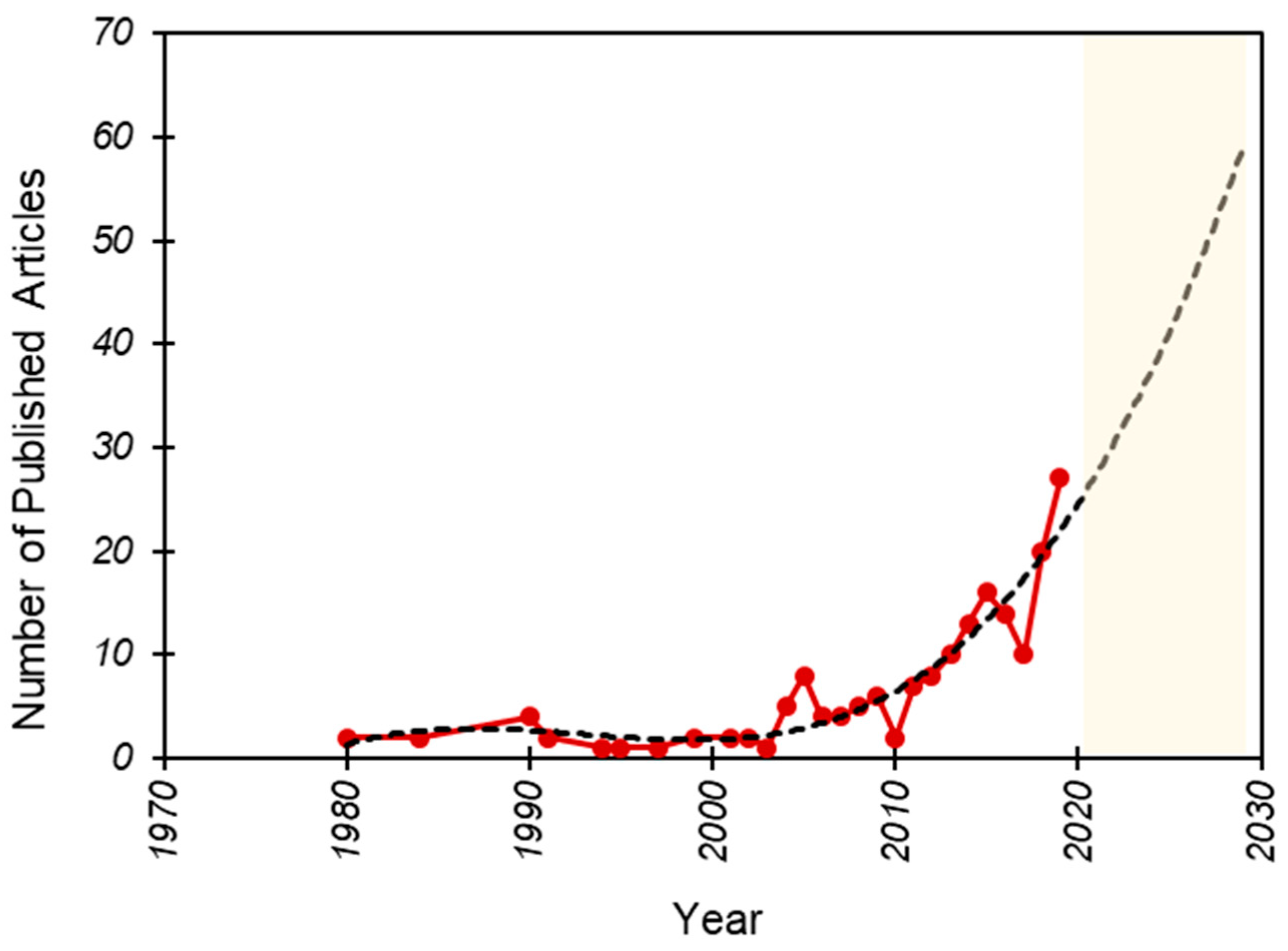
:1. Introduction
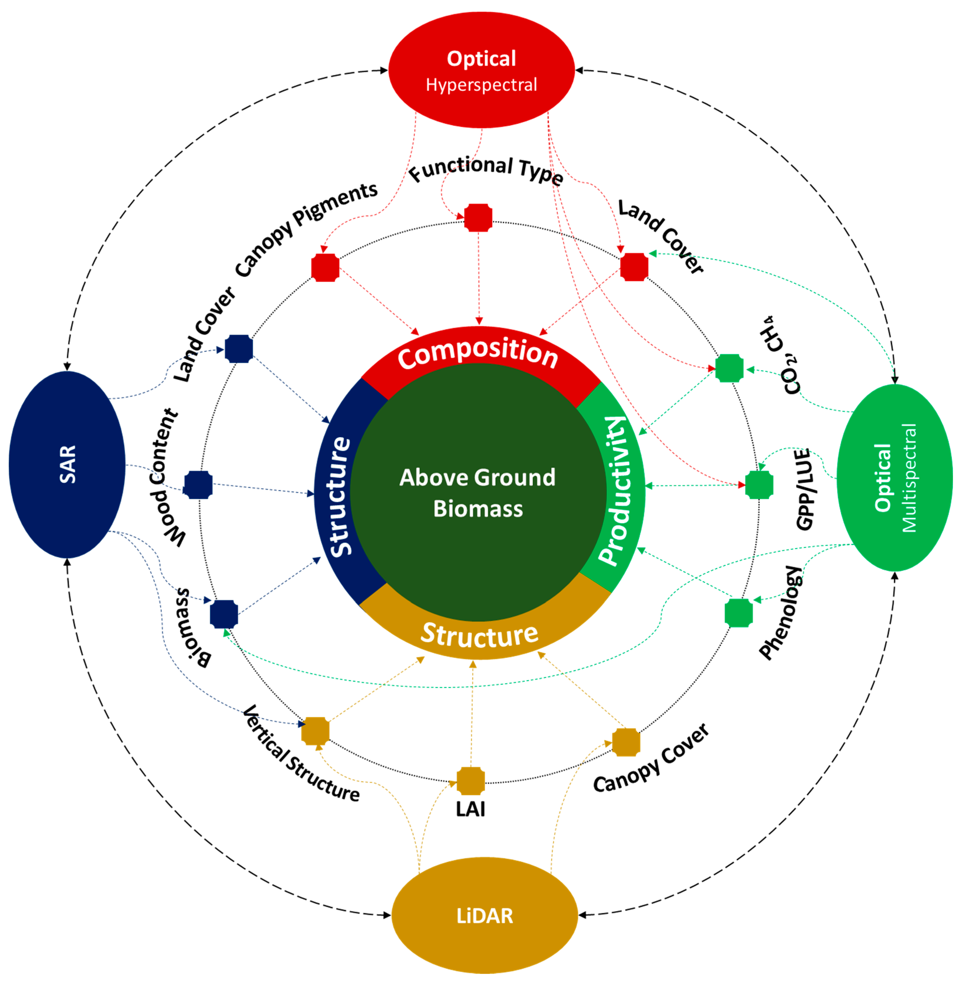
2. Field Inventories and Remote Sensing for Biomass Estimation
3. Mapping of Land Cover and Physiological or Structural Variables
3.1. Land Cover Products
3.2. Physiological Variables
3.2.1. Leaf Area Structure
3.2.2. Canopy Height
3.2.3. Forest Age Class
3.2.4. Phenology Cycle
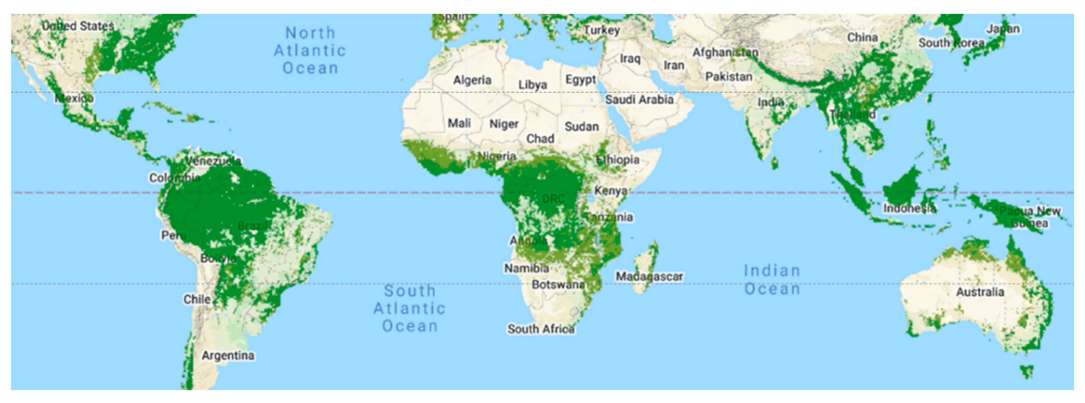
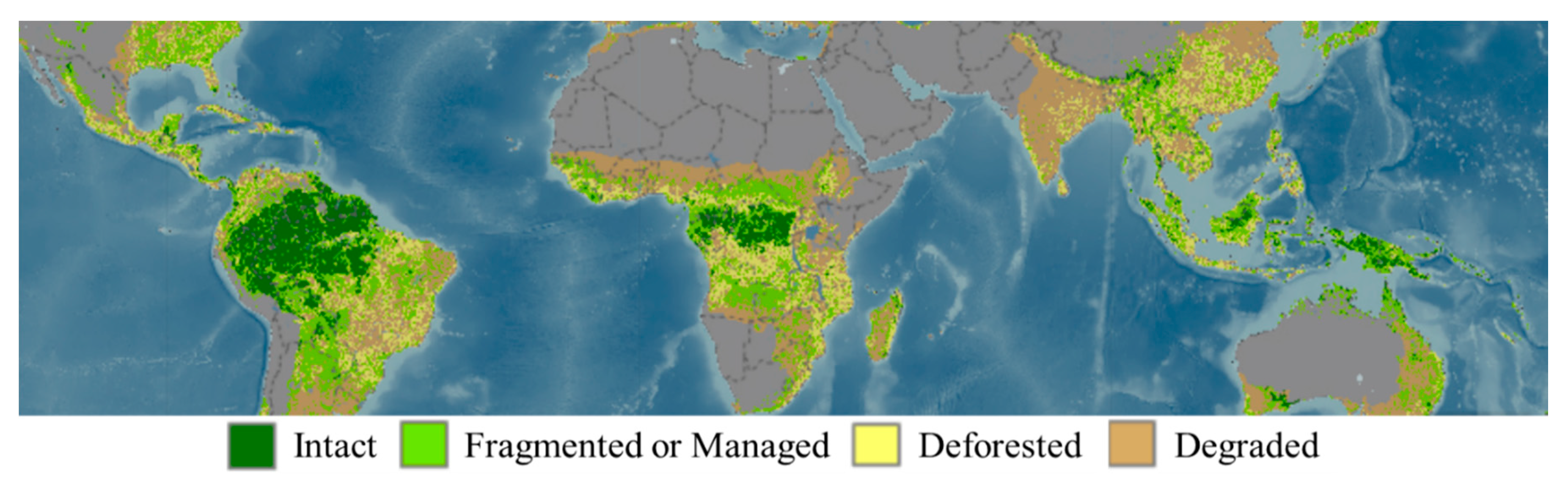
4. Changes in Tropical Forest Cover
5. Tropical Deforestation and Carbon Emissions
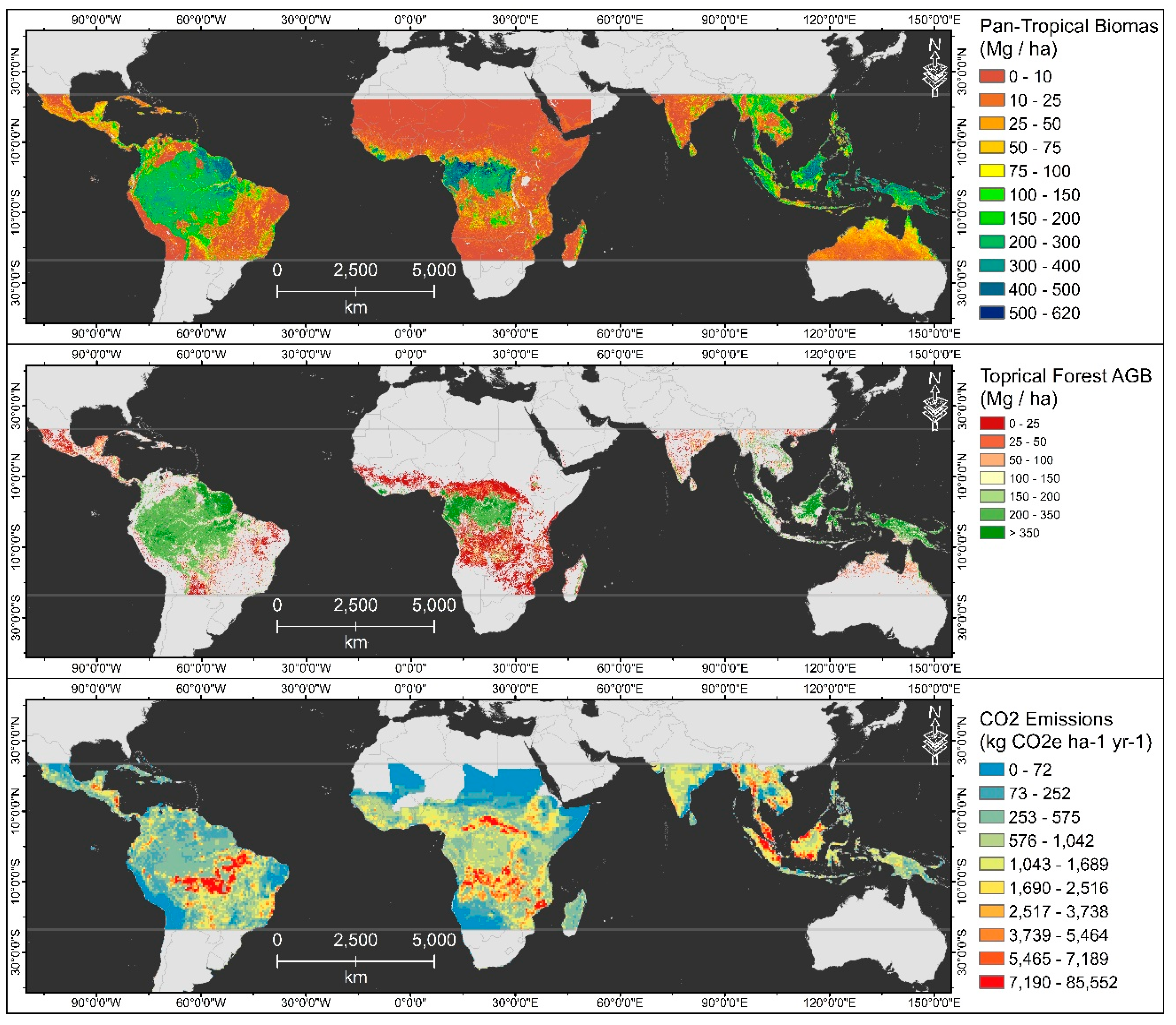
6. Pan-Tropical AGB Mapping
6.1. Country-wide High-Resolution Tropical Biomass Mapping
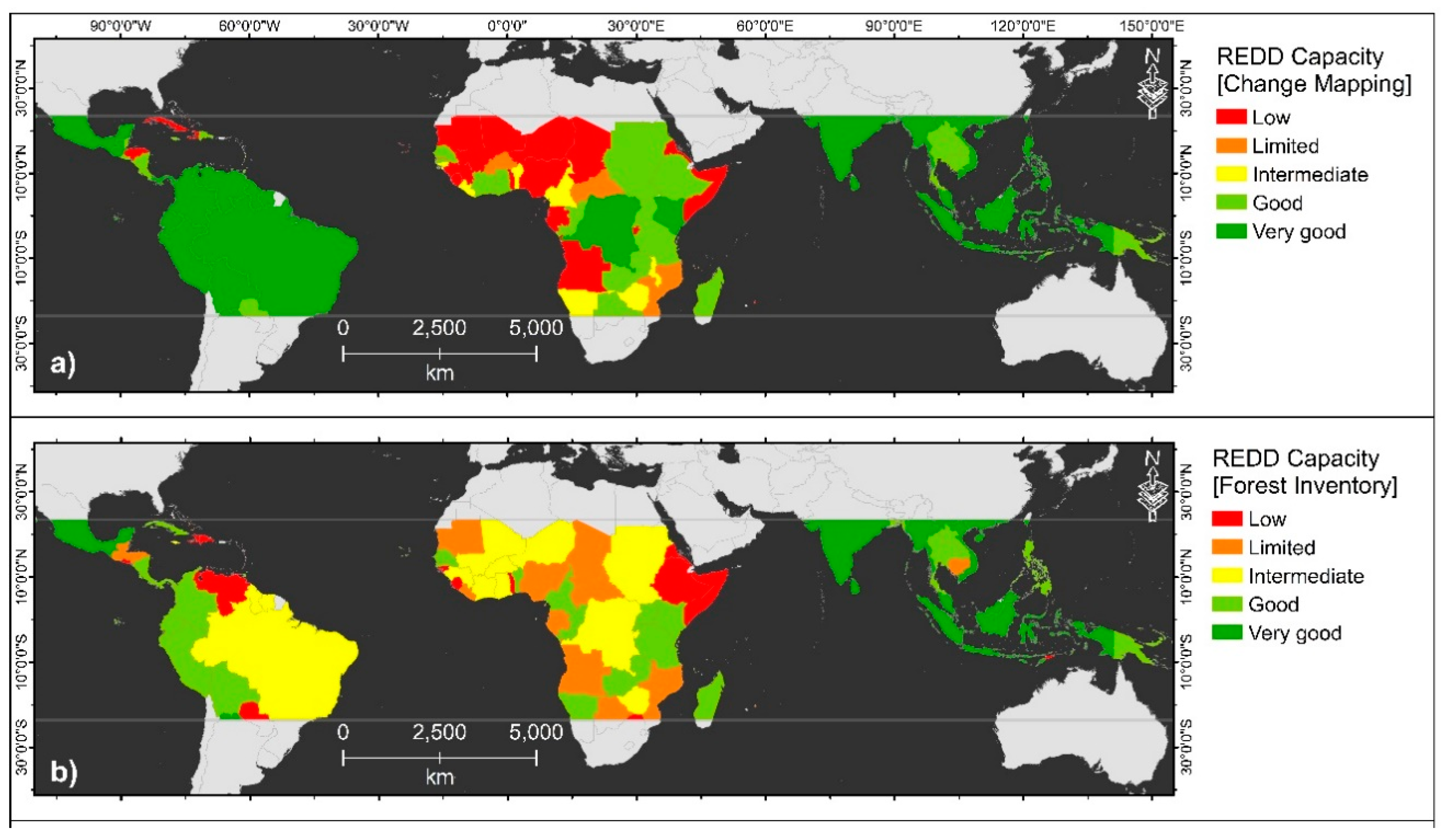
6.2. Concepts, Approaches, Coping Capacities and Limitations
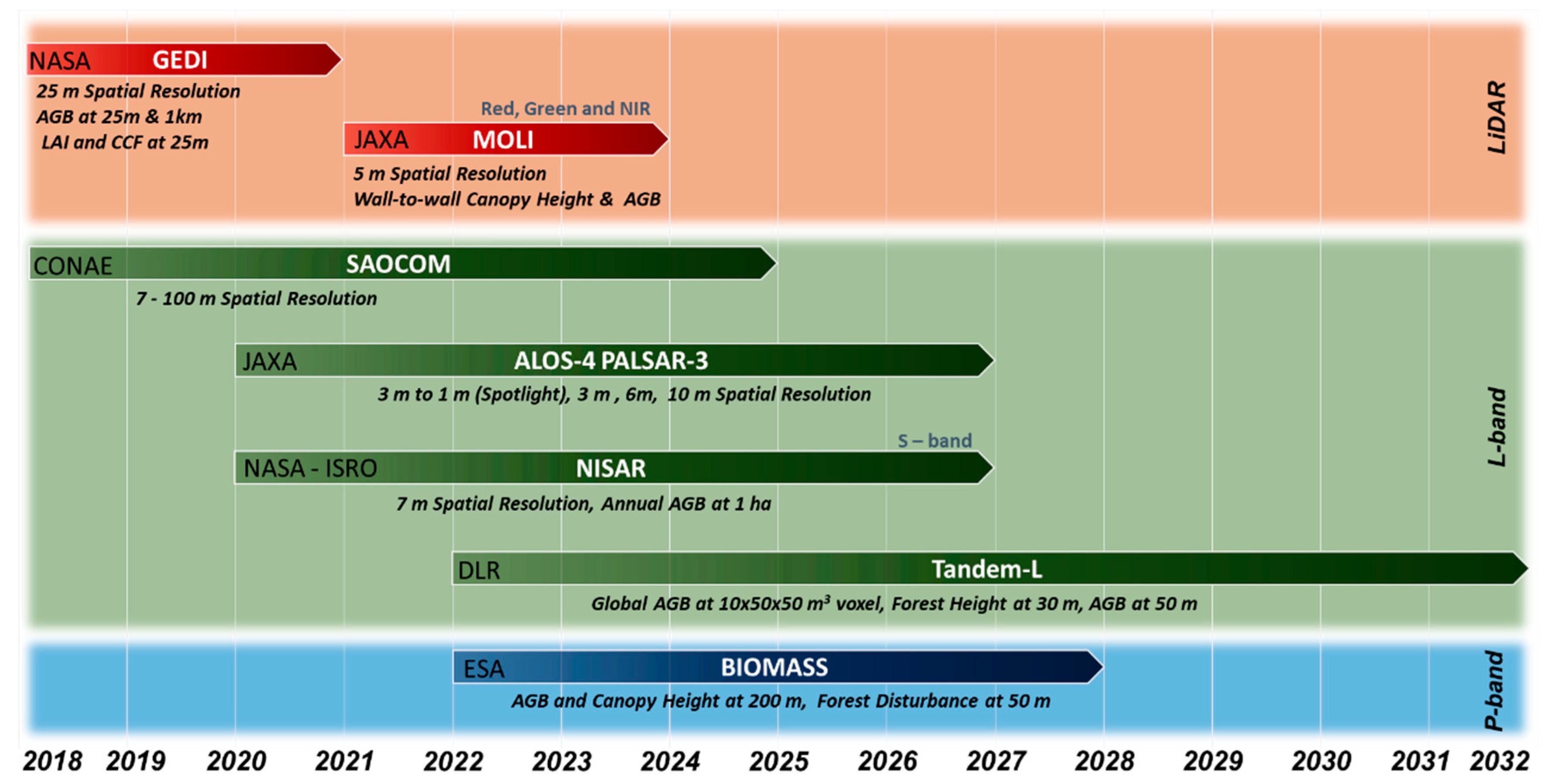
7. Recent and Future Space-Borne Satellite Missions for Biomass Estimation
8. Concluding Remarks
Funding
Acknowledgments
Conflicts of Interest
Appendix A

| Acronym | Definition |
|---|---|
| AGB | Above-Ground Biomass |
| ALOS | Advanced Land Observing Satellite |
| ALS | Airborne Laser Scanning |
| AMSR-E | Advanced Microwave Scanning Radiometer for EOS (AMSR-E) |
| ASA | Argentina’s Space Agency |
| ASAR | Advanced Synthetic Aperture Radar |
| ATLAS | Advanced Topographic Altimeter System |
| AVHRR | Advanced Very High Resolution Radiometer |
| BA | Buenos Aires |
| BEF | Biomass Expansion Factors |
| BGB | Below Ground Biomass |
| CERES | Clouds and the Earth’s Radiant Energy System |
| CLAS | Carnegie Landsat Analysis System |
| CCI | Climate Change Initiative |
| CGLS | Copernicus Global Land Service |
| CGLS-LC100 | Copernicus Global Land Service – Land Cover 100 |
| CIAT | International Center for Tropical Agriculture |
| CONAE | Comisión Nacional de Actividades Espaciales |
| CSA | Canadian Space Agency |
| DBH | diameter at breast height |
| DW | Deadwood |
| DLR | German Aerospace Center |
| EO | Earth Observation |
| ESA | European Space Agency |
| ETM+ | Enhanced Thematic Mapper + |
| EVI | Enhanced Vegetation Index |
| FAO | Food and Agriculture Organization |
| FAPAR | Fraction of Absorbed Photosynthetically Active Radiation |
| FCover | Fraction of Vegetation Cover |
| FORMA | Forest Monitoring for Action |
| FOTO | Fourier-Based Textural Ordination |
| FPAR | Fraction of Photosynthetically Active Radiation |
| FRA | Forest Resources Assessment |
| FREL/FRL | Forest reference emission levels and forest reference levels |
| FVC | Fraction of Vegetation Cover |
| GEDI | Global Ecosystem Dynamics Investigation |
| GEE | Google Earth Engine |
| GEO | Group on Earth Observations |
| GFC | Global Forest Change |
| GFOI | The Global Forest Observations Initiative |
| GFW | Global Forest Watch |
| GHG | Greenhouse gas |
| GIMMS | Global Inventory Modeling and Mapping Studies |
| GLAD | Global Land Analysis and Discovery |
| GLAS | Geoscience Laser Altimeter System |
| GLC | Global Land Cover |
| GLCF | Global Land Cover Facility |
| GMW | Global Mangrove Watch |
| GOFC-GOLD | Global Observation of Forest Cover and Land Dynamics |
| GORT | Geometric Optical-Radiative Transfer |
| GPP | Gross Primary Production |
| GRACE | Gravity Recovery and Climate Experiment |
| GSFC | Goddard Space Flight Center |
| Gt | Gigatons |
| ha | hectare |
| ICESat | Ice, Cloud, and Land Elevation Satellite |
| IFL | Intact Forest Landscapes |
| InSAR | Interferometric synthetic-aperture radar |
| IPCC | Intergovernmental Panel on Climate Change |
| ISRO | Indian Space Research Organization |
| ISS | International Space Station |
| IUCN | International Union for Conservation of Nature |
| JAXA | Japan Aerospace Exploration Agency |
| JERS-1 | Japanese Earth Resources Satellite 1 |
| LAD | Leaf Area Density |
| LAI | Leaf Area Index |
| LAI | Leaf Area Index |
| LC | Land Cover |
| LCLU | Land Cover Land Use |
| LiDAR | Light Detection and Ranging |
| LPDAAC | Land Processes Distributed Active Archive Center |
| LSP | Land Surface Phenology |
| MERIS | Medium Resolution Imaging Spectrometer |
| MMU | Minimum Mapping Unit |
| MODIS | Moderate Resolution Imaging Spectroradiometer |
| MOLI | Multi-footprint Observation LiDAR and Imager |
| MRV | Measuring, Reporting and Verification |
| NASA | National Aeronautics and Space Administration |
| NASG | National Administration of Surveying, Mapping and Geoinformation of China |
| NDVI | Normalized difference vegetation index |
| NEP | Net Ecosystem Production |
| NIR | Near Infrared |
| NISAR | NASA-ISRO SAR |
| NOAA | National Oceanic and Atmospheric Administration |
| NPP | Net Primary Productivity |
| NPP | Net Primary Productivity |
| PALSAR | Phased Array type L-band Synthetic Aperture Radar |
| PAR | Photosynthetically Active Radiation |
| PgC | Petagram of Carbon |
| PROBA-V | Project for On-Board Autonomy—Vegetation |
| PTC | Percent Tree Cover |
| QSCAT | Quick Scatterometer |
| RADAR | Radio Detection and Ranging |
| REDD | Reducing Emissions from Deforestation and Forest Degradation |
| REDD+ | Reducing Emissions from Deforestation and Forest Degradation, and the role of conservation, sustainable management of forests and enhancement of forest carbon stocks in developing countries |
| RMSE | Root Mean Square Error |
| SAOCOM | Argentinean SAtélite Argentino de Observación Con Microondas |
| SAR | Synthetic Aperture Radar |
| SIF | Sun-Induced Chlorophyll Fluorescence |
| SLC | Scan Line Corrector |
| SPOT | Satellite Pour l’Observation de la Terre |
| SRTM | shuttle radar topography mission |
| SVM | Support Vector Machine |
| TLS | Terrestrial Laser Scanning |
| TRMM | Tropical Rainfall Measurement Mission |
| TWS | Terrestrial Water Storage |
| UAV | Unmanned Aerial Vehicle |
| UMD | University of Maryland |
| UNFCCC | United Nations Framework Convention on Climate Change |
| UNSPF | United Nations Strategic Plan for Forests |
| USGS | United States Geological Survey |
| VCF | Vegetation Continuous Fields |
| VFP | Vertical Foliage Profile |
| VOP | Vegetation Optical Depth |
| WRI | World Resources Institute |
| Ecosystem Type | Study Area | Satellite/Sensor | RS Method | Biomass Scale | Accuracy | Resolution | Image Year | Field Data | Publication Year | Reference |
|---|---|---|---|---|---|---|---|---|---|---|
| Tropical savanna | Senegal | NOAA-7 AVHRR | Optical, Field spectrometer | R2 = 0.75 | 1.1 km | 1981 | 194 sites, 1 m2 | 1983 | [198] | |
| Tropical forest | Brazilian Amazon | JERS-1 SAR, NOAA AVHRR | L Band SAR, Optical | 0.05 ha | R2 = 0.30 | 12.5 m | 1993 | 15 site, 10 m by 50 m | 1998 | [199] |
| Tropical forest | Brazilian Amazon | Landsat TM | Optical Multispectral | R2 = 0.37 | 30 m | 1989 to 1995 | 2000 | [200] | ||
| Tropical savanna | Zimbabwe and South Africa | Landsat-5, 7 | Optical Multispectral | R2 = 0.75 to 0.86 | 30 m | 1998, 2000 | 74 sites, 120 × 120 m | 2004 | [201] | |
| Tropical forest savanna | Cameroon, Uganda, Mozambique | ALOS PALSAR | Space-borne L-Band Radar | R2 = 0.61 to 0.76 | 50 m | 2007 | 253 plots | 2009 | [31] | |
| Tropical forest | Brazilian Amazon | Landsat and LiDAR | Airborne LiDAR | 0.1 ha | R2 = 0.80, R2 = 0.84 | 30 m, 1 m | 1999 to 200 | From Literature | 2009 | [33] |
| Tropical forest | Cambodia | ALOS PALSAR | Space-borne L-Band Radar | R2 = 0.64 | 2010 | 40 plots, 30 × 30 m | 2014 | [202] | ||
| Tropical forest | Central Africa | Geoeye-1 and Quickbuird-2 | Optical, Multispectral | 100 m | R2= 0.85 | Sub-meter | 2012 | 474 samples 178 tree species | 2014 | [175] |
| Tropical forest | Southeast Asia | Google Earth™, VHR imagery | Composite RGB, Aerial Multispectral | - | 50 cm, 8 cm | 2012, 2013 | 25 plots of 1 ha | 2015 | [176] | |
| Tropical forest | Inter-Continental | Pleiades images | Multispectral Textural Features | -- | R = −0.42 R = −0.57 R2 = 0.47 | 70 cm to 1 m | 328 plots of 1 ha | 2017 | [177] | |
| Low biomass savanna | Senegal | ALOS-PALSAR SSM/I | RADAR and Brightness Temperature | 10 tons ha−1 | R2 = 0.52 | 150 m, 100 m, 12.5 km | 2006, 2009, 2010 | 48 sites of 50 × 50 m | 2018 | [203] |
| Seasonally dry ecosystems | Southern African | ALOS PALSAR | Space-borne L-Band Radar | ≥10 MgC ha−1 per pixel | R2 = 0.57 | 25 m | 2007–2010 | 137 sites of 0.6 ha | 2018 | [14] |
| Primary and secondary tropical forest | Cambodia | Quickbird-2, LiDAR, Digital orthophotos | Optical Multispectral, ALTM 3100, Aerial Photos | Object-Based | R2 = 0.90, R2 = 0.73 | 0.61–2.44 m, 1 m, 0.5 m | 2011 | 57 sample plots. 30 m × 30 m (38) 50 m × 50 m (19) | 2018 | [174] |
| Mixed tropical forest | Malaysia | TLS and, UAV | Integrated UAV and TLS | 0.16 m2 m−3 | 43% | 10 cm | 60 × 60 m | 2019 | [29] | |
| Tropical rain forest | French Guiana | RIEGL LMS-Q780 sensor | ALS | -- | RMSE = 7.7 | 55–112 points/m2 | 2015 | Six plots of 24,688 trees | 2019 | [20] |
| Tropical forest | Brazilian Amazon | Airborne LiDAR | ALS50-II, ALTM 3100, ALTM Orion, Harrier 68i | -- | R2 =0.8 | 22.7 to 66.4 pts m−2 | 2008–2017 | 2019 | [9] | |
| Regenerated tropical forest | Tanzania | RapidEye | Optical Multispectral | 1 ha | R2 = 0.69 | 5 m | 2010, 2011 | 32,000 plots | 2019 | [173] |
| Tropical lowlands forest | Peru, Amazonian Basin | Planet Dove, LiDAR | Optical Multispectral, LiDAR | -- | R2 = 0.70 | 4 m | 2011, 2013, 2017 | equations developed by [33] | 2019 | [114] |
| Tropical forest | South America | Landsat-8, Sentinel-1, PALSAR, Airborne LiDAR | Optical Multispectral, LiDAR, SAR | -- | R2 = 0.60 to 0.95 | 30 m | 2018 | -- | 2019 | [204] |
| Tropical dry forest | Sudanian Savanna, West Africa | Sentinel—1 and 2 | Multispectral and SAR images | -- | RMSE = 78.6, 60.6, 45.4 | 10 m | 2017 | 218 plots 50 × 20 m | 2020 | [171] |
| Satellite/Sensor | Spatial Resolution (m) | Revisit Time (days) | Spectral Resolution (µm) |
|---|---|---|---|
| Landsat | 15–120 | 16 | 0.45–12.5 (11 bands) |
| SPOT | 10–20 | 26 | 0..45–1.75 (5 bands) |
| MODIS | 250–1000 | 0.25 | 0.4–14.4 (36 bands) |
| Quickbird | 0.61–0.72 | 1-6 | 0.45–0.9 (4 bands) |
| Pleiades | 0.5–2 | 1 | 0.47–0.94 (5 bands) |
| Sentinel-2 | 10–60 | 5 | 0.04–2.19 (12 bands) |
| Sentinel-3 (OLCI) | 300 | 27 | 0.4–1.02 (21 bands) |
| CERES (TRMM) | 10,000 | 46 | 0.3–100 (3 bands) |
| CHRIS | 18-36 | 7 | 0.40–1.05 (19 bands) |
| RapidEye | 5 | 5 | 0.44–0.85 (5 bands) |
| Planet Dove | 4 | 1 | 0.42–0.90 (4 bands) |
| GeoEye | 0.46–1.84 | 2 to 8 | 0.45–0.92 (4 bands) |
| AVHRR | 1100 | Twice daily | 0.58–12.50 (5 bands) |
| MERIS (Envisat-1) | 260 × 300 | 35 | 0.39 to 1.04 (15 bands) |
| Mission | Period | Method | Specification/Products | Agency | Reference |
|---|---|---|---|---|---|
| NISAR | 2021–2026 | L-band | 7 m spatial resolution, Annual AGB map at 1 ha | NASA-ISRO | [117] |
| ALOS-PALSAR | 2006–2012 | L-band | AGB map at 100 m | JAXA | [205] |
| ALOS-2 PALSAR-2 | 2014–2020 | L-band | AGB at 250 m resolution | JAXA | [206] |
| ALOS-4 PALSAR-3 | 2021–2026 | L-band | 3 m × 1 m (Spotlight), 3 m × 3 m, 6 m × 6 m, 10 m × 10 m | JAXA | [194] |
| SAOCOM | 2018–2025 | L-band | 7–100 m spatial resolution | CONAE | [191] |
| Tandem-L | 2022–2032 | L-band | 10 × 50 × 50 m3, Forest Height at 30 m, Forest Biomass at 50 m | DLR | [187] |
| BIOMASS | 2022–2027 | P-band | AGB at 200 m, Canopy Height at 200 m Forest Disturbance at 50 m | ESA | [186] |
| RADARSAT-2 | 2007–2020 | C-Band | 3–100 m Spatial resolution, AGB High-level accuracy of 0.25 ha | CSA | [207] |
| Sentinel-1 | 2014–2026 | C-Band | 5 m × 5 m spatial resolution, Mean AGB 70.38 ton/ha | ESA | [208] |
| GRACE | 2002–2017 | S-Band | Accuracy is sufficient to determine a change in mass equivalent to a volume of water with depth 1 cm over a radius of about 400 km. 30 day revisit. | NASA/DLR | [209] |
| GEDI | 2018–2020 | LiDAR | 25 m footprint, CCF, LAI at 25 m, and AGB at 25 m and 1 km | NASA | [108] |
| MOLI | 2022–2024 | LiDAR, R, G, NIR | 5 m spatial resolution Canopy Height and Forest Biomass Maps | JAXA | [195] |
| ICESat-1 | 2003–2010 | LIDAR | Global forest AGB density was 210.09 Mg/ha on average | NASA/GSFC | [210] |
| ICESat-2 | 2018–2021 | LIDAR | 30 m spatial resolution AGB map, operates at 532 nm wavelength | NASA/GSFC | [211] |
References
- Nobre, C.A.; Sellers, P.J.; Shukla, J. Amazonian deforestation and regional climate change. J. Clim. 1991, 4, 957–988. [Google Scholar] [CrossRef] [Green Version]
- Chazdon, R.L.; Broadbent, E.N.; Rozendaal, D.M.A.; Bongers, F.; Zambrano, A.M.A.; Aide, T.M.; Balvanera, P.; Becknell, J.M.; Boukili, V.; Brancalion, P.H.S.; et al. Carbon sequestration potential of second-growth forest regeneration in the Latin American tropics. Sci. Adv. 2016, 2, e1501639. [Google Scholar] [CrossRef] [PubMed] [Green Version]
- Federici, S.; Tubiello, F.N.; Salvatore, M.; Jacobs, H.; Schmidhuber, J. New estimates of CO2 forest emissions and removals: 1990–2015. For. Ecol. Manag. 2015, 352, 89–98. [Google Scholar] [CrossRef] [Green Version]
- Pan, Y.; Birdsey, R.A.; Fang, J.; Houghton, R.; Kauppi, P.E.; Kurz, W.A.; Phillips, O.L.; Shvidenko, A.; Lewis, S.L.; Canadell, J.G.; et al. A large and persistent carbon sink in the world’s forests. Science 2011, 333, 988–993. [Google Scholar] [CrossRef] [Green Version]
- FAO. Global Forest Resource Assessment; FAO: Rome, Italy, 2010. [Google Scholar]
- FAO. Global Forest Resources Assessment 2020: Main Report; FAO: Remote, Italy, 2020; ISBN 978-92-5-132974-0. [Google Scholar]
- Stephens, B.B.; Gurney, K.R.; Tans, P.P.; Sweeney, C.; Peters, W.; Bruhwiler, L.; Ciais, P.; Ramonet, M.; Bousquet, P.; Nakazawa, T.; et al. Weak northern and strong tropical land carbon uptake from vertical profiles of atmospheric CO2. Science 2007, 316, 1732–1735. [Google Scholar] [CrossRef] [Green Version]
- Lewis, S.L.; Lopez-Gonzalez, G.; Sonké, B.; Affum-Baffoe, K.; Baker, T.R.; Ojo, L.O.; Phillips, O.L.; Reitsma, J.M.; White, L.; Comiskey, J.A.; et al. Increasing carbon storage in intact African tropical forests. Nature 2009, 457, 1003. [Google Scholar] [CrossRef]
- Shao, G.; Stark, S.C.; de Almeida, D.R.A.; Smith, M.N. Towards high throughput assessment of canopy dynamics: The estimation of leaf area structure in Amazonian forests with multitemporal multi-sensor airborne lidar. Remote Sens. Environ. 2019, 221, 1–13. [Google Scholar] [CrossRef]
- Chapin, F.S.; Matson, P.A.; Vitousek, P.M. Principles of Terrestrial Ecosystem Ecology; Springer: New York, NY, USA, 2011; ISBN 978-1-4419-9503-2. [Google Scholar]
- Laurance, W.F. Gaia’s Lungs: Are rainforests inhaling Earth’s excess carbon dioxide? Nat. Hist. 1999, 108, 96. [Google Scholar]
- Abbas, S.; Nichol, J.E.; Fischer, G.A. A 70-year perspective on tropical forest regeneration. Sci. Total Environ. 2016, 544, 544–552. [Google Scholar] [CrossRef]
- Abbas, S.; Nichol, J.E.; Zhang, J.; Fischer, G.A. The accumulation of species and recovery of species composition along a 70 year succession in a tropical secondary forest. Ecol. Indic. 2019, 106, 105524. [Google Scholar] [CrossRef]
- McNicol, I.M.; Ryan, C.M.; Mitchard, E.T.A. Carbon losses from deforestation and widespread degradation offset by extensive growth in African woodlands. Nat. Commun. 2018, 9, 3045. [Google Scholar] [CrossRef] [PubMed]
- Kim, D.; Sexton, J.O.; Townshend, J.R. Accelerated deforestation in the humid tropics from the 1990s to the 2000s. Geophys. Res. Lett. 2015, 42, 1–7. [Google Scholar] [CrossRef] [PubMed]
- Geist, H.J.; Lambin, E.F. Proximate causes and underlying driving forces of tropical deforestation. Bioscience 2002, 52, 143. [Google Scholar] [CrossRef]
- Wright, S.J. Tropical forests in a changing environment. Trends Ecol. Evol. 2005, 20, 553–560. [Google Scholar] [CrossRef] [PubMed]
- Boisvenue, C.; White, J.C. Information needs of next-generation forest carbon models: Opportunities for remote sensing science. Remote Sens. 2019, 11, 463. [Google Scholar] [CrossRef] [Green Version]
- Saukkola, A.; Melkas, T.; Riekki, K.; Sirparanta, S.; Peuhkurinen, J.; Holopainen, M.; Hyyppä, J.; Vastaranta, M. Predicting forest inventory attributes using airborne laser scanning, aerial imagery, and harvester data. Remote Sens. 2019, 11, 797. [Google Scholar] [CrossRef] [Green Version]
- Aubry-Kientz, M.; Dutrieux, R.; Ferraz, A.; Saatchi, S.; Hamraz, H.; Williams, J.; Coomes, D.; Piboule, A.; Vincent, G. A comparative assessment of the performance of individual tree crowns delineation algorithms from ALS data in tropical forests. Remote Sens. 2019, 11, 1086. [Google Scholar] [CrossRef] [Green Version]
- Kindermann, G.E.; McCallum, I.; Fritz, S.; Obersteiner, M. A global forest growing stock, biomass and carbon map based on FAO statistics. Silva Fenn. 2008, 42, 387–396. [Google Scholar] [CrossRef] [Green Version]
- MacDicken, K.; Reams, G.; de Freitas, J. Introduction to the changes in global forest resources from 1990 to 2015. For. Ecol. Manag. 2015, 352, 1–2. [Google Scholar] [CrossRef]
- Herold, M.; Carter, S.; Avitabile, V.; Espejo, A.B.; Jonckheere, I.; Lucas, R.; McRoberts, R.E.; Næsset, E.; Nightingale, J.; Petersen, R.; et al. The role and need for space-based forest biomass-related measurements in environmental management and policy. Surv. Geophys. 2019, 40, 757–778. [Google Scholar] [CrossRef] [Green Version]
- Segura, M.; Kanninen, M. Allometric models for tree volume and total aboveground biomass in a tropical humid forest in Costa Rica1. Biotropica 2005, 37, 2–8. [Google Scholar] [CrossRef]
- Henry, M.; Picard, N.; Trotta, C.; Manlay, R.J.; Valentini, R.; Bernoux, M.; Saint-André, L. Estimating tree biomass of Sub-Saharan African forests: A review of available allometric equations. Silva Fenn. 2011, 45, 477–569. [Google Scholar] [CrossRef] [Green Version]
- Popkin, G. The hunt for the world’s missing carbon. Nature 2015, 523, 20–22. [Google Scholar] [CrossRef] [PubMed]
- Kumar, L.; Sinha, P.; Taylor, S.; Alqurashi, A.F. Review of the use of remote sensing for biomass estimation to support renewable energy generation. J. Appl. Remote Sens. 2015, 9, 097696. [Google Scholar] [CrossRef]
- Dube, T.; Mutanga, O.; Shoko, C.; Samuel, A.; Bangira, T. Remote sensing of aboveground forest biomass: A review. Trop. Ecol. 2016, 57, 125–132. [Google Scholar]
- Schneider, F.D.; Kükenbrink, D.; Schaepman, M.E.; Schimel, D.S.; Morsdorf, F. Quantifying 3D structure and occlusion in dense tropical and temperate forests using close-range LiDAR. Agric. For. Meteorol. 2019, 268, 249–257. [Google Scholar] [CrossRef]
- Patenaude, G.; Milne, R.; Dawson, T.P. Synthesis of remote sensing approaches for forest carbon estimation: Reporting to the Kyoto Protocol. Environ. Sci. Policy 2005, 8, 161–178. [Google Scholar] [CrossRef]
- Mitchard, E.T.A.; Saatchi, S.S.; Woodhouse, I.H.; Nangendo, G.; Ribeiro, N.S.; Williams, M.; Ryan, C.M.; Lewis, S.L.; Feldpausch, T.R.; Meir, P. Using satellite radar backscatter to predict above-ground woody biomass: A consistent relationship across four different African landscapes. Geophys. Res. Lett. 2009, 36, 1–6. [Google Scholar] [CrossRef]
- Asner, G.P.; Brodrick, P.G.; Philipson, C.; Vaughn, N.R.; Martin, R.E.; Knapp, D.E.; Heckler, J.; Evans, L.J.; Jucker, T.; Goossens, B.; et al. Mapped aboveground carbon stocks to advance forest conservation and recovery in Malaysian Borneo. Biol. Conserv. 2018, 217, 289–310. [Google Scholar] [CrossRef]
- Asner, G.P. Tropical forest carbon assessment: Integrating satellite and airborne mapping approaches. Environ. Res. Lett. 2009, 4, 03409. [Google Scholar] [CrossRef]
- Asner, G.P.; Knapp, D.E.; Martin, R.E.; Tupayachi, R.; Anderson, C.B.; Mascaro, J.; Sinca, F.; Chadwick, K.D.; Higgins, M.; Farfan, W.; et al. Targeted carbon conservation at national scales with high-resolution monitoring. Proc. Natl. Acad. Sci. USA 2014, 111, E5016–E5022. [Google Scholar] [CrossRef] [PubMed] [Green Version]
- Asner, G.P. Selective logging in the Brazilian Amazon. Science 2005, 310, 480–482. [Google Scholar] [CrossRef] [PubMed]
- Smith, J.E.; Heath, L.S.; Woodbury, P.B. How to estimate forest carbon for large areas from inventory data. J. For. 2004, 102, 25–31. [Google Scholar]
- Xiao, X.; Hagen, S.; Zhang, Q.; Keller, M.; Moore, B. Detecting leaf phenology of seasonally moist tropical forests in South America with multi-temporal MODIS images. Remote Sens. Environ. 2006, 103, 465–473. [Google Scholar] [CrossRef]
- Chave, J.; Andalo, C.; Brown, S.; Cairns, M.A.; Chambers, J.Q.; Eamus, D.; Fölster, H.; Fromard, F.; Higuchi, N.; Kira, T.; et al. Tree allometry and improved estimation of carbon stocks and balance in tropical forests. Oecologia 2005, 145, 87–99. [Google Scholar] [CrossRef] [PubMed]
- Condit, R. Methods for estimating above-ground biomass of forest and replacement vegetation in the tropics. Cent. Trop. For. Sci. Res. Man. 2008, 25, 73. [Google Scholar]
- Picard, N.; Saint-André, L.; Henry, M. Manual for Building Tree Volume and Biomass Allometric Equations: From Field Measurement to Prediction; Food and Agricultural Organization of the United Nations: Rome, Italy; Centre de Coopération Internationale en Recherche Agronomique pour le Développement: Montpeiller, France, 2012; ISBN 9789251073476. [Google Scholar]
- Specht, A.; West, P.W. Estimation of biomass and sequestered carbon on farm forest plantations in northern New South Wales, Australia. Biomass Bioenergy 2003, 25, 363–379. [Google Scholar] [CrossRef]
- Hunter, M.O.; Keller, M.; Victoria, D.; Morton, D.C. Tree height and tropical forest biomass estimation. Biogeosciences 2013, 10, 8385–8399. [Google Scholar] [CrossRef] [Green Version]
- Clark, D.B.; Kellner, J.R. Tropical forest biomass estimation and the fallacy of misplaced concreteness. J. Veg. Sci. 2012, 23, 1191–1196. [Google Scholar] [CrossRef]
- Lu, D.; Chen, Q.; Wang, G.; Liu, L.; Li, G.; Moran, E. A survey of remote sensing-based aboveground biomass estimation methods in forest ecosystems. Int. J. Digit. Earth 2016, 9, 63–105. [Google Scholar] [CrossRef]
- Masek, J.G.; Hayes, D.J.; Joseph Hughes, M.; Healey, S.P.; Turner, D.P. The role of remote sensing in process-scaling studies of managed forest ecosystems. For. Ecol. Manag. 2015, 355, 109–123. [Google Scholar] [CrossRef] [Green Version]
- Xiao, J.; Chevallier, F.; Gomez, C.; Guanter, L.; Hicke, J.A.; Huete, A.R.; Ichii, K.; Ni, W.; Pang, Y.; Rahman, A.F.; et al. Remote sensing of the terrestrial carbon cycle: A review of advances over 50 years. Remote Sens. Environ. 2019, 233, 111383. [Google Scholar] [CrossRef]
- Turner, D.P.; Ollinger, S.V.; Kimball, J.S. Integrating Remote Sensing and Ecosystem Process Models for Landscape- to Regional-Scale Analysis of the Carbon Cycle. Bioscience 2006, 54, 573. [Google Scholar] [CrossRef] [Green Version]
- Ciais, P.; Sabine, C.; Bala, G.; Bopp, L.; Brovkin, V.; Canadell, J.; Chhabra, A.; DeFries, R.; Galloway, J.; Heimann, M.; et al. Carbon and Other Biogeochemical Cycles. In Climate Change 2013—The Physical Science Basis; Intergovernmental Panel on Climate Change, Ed.; Cambridge University Press: Cambridge, UK, 2013; Volume 9781107057, pp. 465–570. ISBN 9781107415324. [Google Scholar]
- Quéré, C.; Andrew, R.; Friedlingstein, P.; Sitch, S.; Hauck, J.; Pongratz, J.; Pickers, P.; Ivar Korsbakken, J.; Peters, G.; Canadell, J.; et al. Global carbon budget 2018. Earth Syst. Sci. Data 2018, 10, 2141–2194. [Google Scholar] [CrossRef] [Green Version]
- Quijas, S.; Boit, A.; Thonicke, K.; Murray-Tortarolo, G.; Mwampamba, T.; Skutsch, M.; Simoes, M.; Ascarrunz, N.; Peña-Claros, M.; Jones, L.; et al. Modelling carbon stock and carbon sequestration ecosystem services for policy design: A comprehensive approach using a dynamic vegetation model. Ecosyst. People 2018, 15, 42–60. [Google Scholar] [CrossRef] [Green Version]
- Merrick, T.; Pau, S.; Jorge, M.L.S.; Bennartz, R.; Silva, T.S. Spatiotemporal patterns and phenology of tropical vegetation solar-induced chlorophyll fluorescence across Brazilian biomes using satellite observations. Remote Sens. 2019, 11, 1746. [Google Scholar] [CrossRef] [Green Version]
- Jensen, J.R. Remote Sensing of the Environment: An Earth Resource Perspective, 2nd ed.; Pearson Education India: Bengaluru, India, 2009. [Google Scholar]
- Harrison, S.P.; Gaillard, M.-J.; Stocker, B.D.; Vander Linden, M.; Klein Goldewijk, K.; Boles, O.; Braconnot, P.; Dawson, A.; Fluet-Chouinard, E.; Kaplan, J.O.; et al. Development and testing scenarios for implementing land use and land cover changes during the Holocene in Earth system model experiments. Geosci. Model Dev. 2020, 13, 805–824. [Google Scholar] [CrossRef] [Green Version]
- Smith, M.C.; Singarayer, J.S.; Valdes, P.J.; Kaplan, J.O.; Branch, N.P. The biogeophysical climatic impacts of anthropogenic land use change during the Holocene. Clim. Past 2016, 12, 923–941. [Google Scholar] [CrossRef] [Green Version]
- Buchhorn, M.; Smets, B.; Bertels, L.; Lesiv, M.; Tsendbazar, N.-E.; Herold, M.; Fritz, S. Copernicus Global Land Service: Land Cover 100m: Epoch 2015: Globe; OpenAIRE: Genève, Switzerland, 2019. [Google Scholar] [CrossRef]
- Ma, W.; Domke, G.M.; Woodall, C.W.; Amato, A.W.D. Land use changes, disturbances, and their interactions on future forest aboveground biomass dynamics in the Northern US. Forests 2019, 10, 606. [Google Scholar] [CrossRef] [Green Version]
- Cracknell, A.P. The exciting and totally unanticipated success of the AVHRR in applications for which it was never intended. Adv. Space Res. 2001, 28, 233–240. [Google Scholar] [CrossRef]
- Tucker, C.; Pinzon, J.; Brown, M.; Slayback, D.; Pak, E.; Mahoney, R.; Vermote, E.; El Saleous, N. An extended AVHRR 8-km NDVI dataset compatible with MODIS and SPOT vegetation NDVI data. Int. J. Remote Sens. 2005, 26, 4485–4498. [Google Scholar] [CrossRef]
- Minnemeyer, S.; Laestadius, L.; Sizer, N.; Saint-Laurent, C.; Potapov, P. The Atlas of Forest Landscape Restoration Opportunities; World Resources Institute: Washington, DC, USA; Available online: http://www.wri.org/applications/maps/flr-atlas/# (accessed on 5 August 2019).
- Hansen, M.C.; DeFries, R.S.; Townshend, J.R.G.; Carroll, M.; Dimiceli, C.; Sohlberg, R.A. Global Percent Tree Cover at a Spatial Resolution of 500 Meters: First Results of the MODIS Vegetation Continuous Fields Algorithm. Earth Interact. 2003, 7, 1–15. [Google Scholar] [CrossRef] [Green Version]
- Nguyen, T.H.; Jones, S.; Soto-Berelov, M.; Haywood, A.; Hislop, S. Landsat time-series for estimating forest aboveground biomass and its dynamics across space and time: A review. Remote Sens. 2019, 12, 98. [Google Scholar] [CrossRef] [Green Version]
- GFW Global Forest Watch. Available online: https://www.globalforestwatch.org/ (accessed on 15 September 2019).
- Hansen, M.C.; Krylov, A.; Tyukavina, A.; Potapov, P.V.; Turubanova, S.; Zutta, B.; Ifo, S.; Margono, B.; Stolle, F.; Moore, R. Humid tropical forest disturbance alerts using Landsat data. Environ. Res. Lett. 2016, 11, 034008. [Google Scholar] [CrossRef]
- Hammer, D.; Kraft, R.; Wheeler, D. Alerts of forest disturbance from MODIS imagery. Int. J. Appl. Earth Obs. Geoinf. 2014, 33, 1–9. [Google Scholar] [CrossRef]
- Wheeler, D.; Guzder-Williams, B.; Petersen, R.; Thau, D. Rapid MODIS-based detection of tree cover loss. Int. J. Appl. Earth Obs. Geoinf. 2018, 69, 78–87. [Google Scholar] [CrossRef]
- Reymondin, L.; Jarvis, A.; Perez-Uribe, A.; Touval, J.; Argote, K.; Coca, A.; Rebetez, J.; Guevara, E.; Mulligan, M. Terra-i: A methodology for near real-time monitoring of habitat change at continental scales using MODIS-NDVI and TRMM. Submitt. Remote Sens. Environ. 2012. Available online: http://terra-i.org/dms/docs/reports/Terra-i-Method/Terra-i%20Method.pdf (accessed on 13 September 2020).
- Hansen, M.C.; Potapov, P.V.; Moore, R.; Hancher, M.; Turubanova, S.A.; Tyukavina, A.; Thau, D.; Stehman, S.V.; Goetz, S.J.; Loveland, T.R.; et al. High-resolution global maps of 21st-century forest cover change. Science 2013, 342, 850–853. [Google Scholar] [CrossRef] [Green Version]
- Turubanova, S.; Potapov, P.V.; Tyukavina, A.; Hansen, M.C. Ongoing primary forest loss in Brazil, Democratic Republic of the Congo, and Indonesia. Environ. Res. Lett. 2018, 13, 074028. [Google Scholar] [CrossRef] [Green Version]
- Buchhorn, M.; Smets, B.; Bertels, L.; Lesiv, M.; Tsendbazar, N.-E. Copernicus Global Land Operations “ ‘Vegetation and Energy’ ”CGLOPS-1” Framework Service Contract N° 199494 (JRC), MODERATE DYNAMIC LAND COVER 100M VERSION 2; Joint Research Centre: Ispra, Italy, 2018; ISBN 2008081120080. [Google Scholar]
- Buchhorn, M.; Lesiv, M.; Tsendbazar, N.-E.; Herold, M.; Bertels, L.; Smets, B. Copernicus global land cover layers—Collection 2. Remote Sens. 2020, 12, 1044. [Google Scholar] [CrossRef] [Green Version]
- Silva Junior, C.H.L.; Heinrich, V.H.A.; Freire, A.T.G.; Broggio, I.S.; Rosan, T.M.; Doblas, J.; Anderson, L.O.; Rousseau, G.X.; Shimabukuro, Y.E.; Silva, C.A.; et al. Benchmark maps of 33 years of secondary forest age for Brazil. Zenodo 2020, 7, 1–9. [Google Scholar]
- Hirschmugl, M.; Deutscher, J.; Sobe, C.; Bouvet, A.; Mermoz, S.; Schardt, M. Use of SAR and optical time series for tropical forest disturbance mapping. Remote Sens. 2020, 12, 727. [Google Scholar] [CrossRef] [Green Version]
- Vargas, C.; Montalban, J.; Leon, A.A. Early warning tropical forest loss alerts in Peru using Landsat. Environ. Res. Commun. 2019, 1, 121002. [Google Scholar] [CrossRef]
- Laestadius, L.; Maginnis, S.; Minnemeyer, S.; Potapov, P.; Saint-Laurent, C.; Sizer, N. Mapping opportunities for forest landscape restoration. Unasylva 2011, 62, 1–3. [Google Scholar]
- Bunting, P.; Rosenqvist, A.; Lucas, R.; Rebelo, L.-M.; Hilarides, L.; Thomas, N.; Hardy, A.; Itoh, T.; Shimada, M.; Finlayson, C. The global mangrove watch—A new 2010 global baseline of mangrove extent. Remote Sens. 2018, 10, 1669. [Google Scholar] [CrossRef] [Green Version]
- Shimada, M.; Itoh, T.; Motooka, T.; Watanabe, M.; Shiraishi, T.; Thapa, R.; Lucas, R. New global forest/non-forest maps from ALOS PALSAR data (2007–2010). Remote Sens. Environ. 2014, 155, 13–31. [Google Scholar] [CrossRef]
- Chapter 12—Fractional Vegetation Cover. In Advanced Remote Sensing, 2nd ed.; Liang, S.; Wang, J. (Eds.) Academic Press: Cambridge, MA, USA, 2020; pp. 477–510. ISBN 978-0-12-815826-5. [Google Scholar]
- Baret, F.; Weiss, M.; Verger, A.; Smets, B. Exploiting, Implementing Multi-Scale Agricultural Indicators Sentinels: ATBD for LAI, FAPAR and FCOVER from PROBA-V products at 300m resolution (GEOV3); Imagine Publishing: Bournemouth, UK, 2016. [Google Scholar]
- Chavana-Bryant, C.; Malhi, Y.; Wu, J.; Asner, G.P.; Anastasiou, A.; Enquist, B.J.; Cosio Caravasi, E.G.; Doughty, C.E.; Saleska, S.R.; Martin, R.E.; et al. Leaf aging of Amazonian canopy trees as revealed by spectral and physiochemical measurements. New Phytol. 2017, 214, 1049–1063. [Google Scholar] [CrossRef] [Green Version]
- Wu, J.; Kobayashi, H.; Stark, S.C.; Meng, R.; Guan, K.; Tran, N.N.; Gao, S.; Yang, W.; Restrepo-coupe, N.; Miura, T.; et al. Biological processes dominate seasonality of remotely sensed canopy greenness in an Amazon evergreen forest. New. Phytol. 2018, 217, 1507–1520. [Google Scholar] [CrossRef] [Green Version]
- Guan, K.; Pan, M.; Li, H.; Wolf, A.; Wu, J.; Medvigy, D.; Caylor, K.K.; Sheffield, J.; Wood, E.F.; Malhi, Y.; et al. Photosynthetic seasonality of global tropical forests constrained by hydroclimate. Nat. Geosci. 2015, 8, 284–289. [Google Scholar] [CrossRef]
- Potapov, P.; Yaroshenko, A.; Turubanova, S.; Dubinin, M.; Laestadius, L.; Thies, C.; Aksenov, D.; Egorov, A.; Yesipova, Y.; Glushkov, I.; et al. Mapping the World’ s Intact Forest Landscapes by Remote Sensing. Ecol. Soc. 2008, 13, 51. [Google Scholar] [CrossRef] [Green Version]
- Potapov, P.; Hansen, M.C.; Laestadius, L.; Turubanova, S.; Yaroshenko, A.; Thies, C.; Smith, W.; Zhuravleva, I.; Komarova, A.; Minnemeyer, S.; et al. The last frontiers of wilderness: Tracking loss of intact forest landscapes from 2000 to 2013. Sci. Adv. 2017, 3, e1600821. [Google Scholar] [CrossRef] [PubMed] [Green Version]
- Jun, C.; Ban, Y.; Li, S. Open access to Earth land-cover map. Nature 2014, 514, 434. [Google Scholar] [CrossRef] [PubMed] [Green Version]
- DiMiceli, C.M.; Carroll, M.L.; Sohlberg, R.A.; Huang, C.; Hansen, M.C.; Townshend, J.R.G. Annual Global Automated MODIS Vegetation Continuous Fields (MOD44B) at 250 m Spatial Resolution for Data Years Beginning Day 65, 2000–2010; University of Maryland: College Park, MD, USA, 2017. [Google Scholar]
- GeoVille Global Land Cover Dynamics 2016—2018. Sentinel-2 Time Series Analysis. Available online: https://landmonitoring.earth/portal/ (accessed on 5 August 2019).
- Zhang, X.; Liu, L.; Yan, D. Comparisons of global land surface seasonality and phenology derived from AVHRR, MODIS, and VIIRS data. J. Geophys. Res. Biogeosci. 2017, 122, 1506–1525. [Google Scholar] [CrossRef]
- Townshend, J.R.G.; Carroll, M.; Dimiceli, C.; Sohlberg, R.; Hansen, M.; DeFries, R. Vegetation Continuous Fields MOD44B, 2001 Percent Tree Cover, Collection 5; University of Maryland: College Park, MD, USA, 2011. [Google Scholar]
- Sexton, J.O.; Song, X.P.; Feng, M.; Noojipady, P.; Anand, A.; Huang, C.; Kim, D.H.; Collins, K.M.; Channan, S.; DiMiceli, C.; et al. Global, 30-m resolution continuous fields of tree cover: Landsat-based rescaling of MODIS vegetation continuous fields with lidar-based estimates of error. Int. J. Digit. Earth 2013, 6, 427–448. [Google Scholar] [CrossRef] [Green Version]
- Hansen, M.C.; Stehman, S.V.; Potapov, P.V.; Loveland, T.R.; Townshend, J.R.G.; DeFries, R.S.; Pittman, K.W.; Arunarwati, B.; Stolle, F.; Steininger, M.K.; et al. Humid tropical forest clearing from 2000 to 2005 quantified by using multitemporal and multiresolution remotely sensed data. Proc. Natl. Acad. Sci. USA 2008, 105, 9439–9444. [Google Scholar] [CrossRef] [PubMed] [Green Version]
- Hansen, A.J.; Burns, P.; Ervin, J.; Goetz, S.J.; Hansen, M.; Venter, O.; Watson, J.E.M.; Jantz, P.A.; Virnig, A.L.S.; Barnett, K.; et al. A policy-driven framework for conserving the best of Earth’s remaining moist tropical forests. Nat. Ecol. Evol. 2020, 4, 1377–1384. [Google Scholar] [CrossRef]
- Harris, N.L.; Brown, S.; Hagen, S.C.; Saatchi, S.S.; Petrova, S.; Salas, W.; Hansen, M.C.; Potapov, P.V.; Lotsch, A. Baseline map of carbon emissions from deforestation in tropical regions. Science 2012, 336, 1573–1576. [Google Scholar] [CrossRef] [PubMed]
- DeFries, R.S.; Houghton, R.A.; Hansen, M.C.; Field, C.B.; Skole, D.; Townshend, J. Carbon emissions from tropical deforestation and regrowth based on satellite observations for the 1980s and 1990s. Proc. Natl. Acad. Sci. 2002, 99, 14256–14261. [Google Scholar] [CrossRef] [Green Version]
- Breda, N.J.J. Ground-based measurements of leaf area index: A review of methods, instruments and current controversies. J. Exp. Bot. 2003, 54, 2403–2417. [Google Scholar] [CrossRef]
- Stark, S.C.; Leitold, V.; Wu, J.L.; Hunter, M.O.; de Castilho, C.V.; Costa, F.R.C.; McMahon, S.M.; Parker, G.G.; Shimabukuro, M.T.; Lefsky, M.A.; et al. Amazon forest carbon dynamics predicted by profiles of canopy leaf area and light environment. Ecol. Lett. 2012, 15, 1406–1414. [Google Scholar] [CrossRef] [Green Version]
- Watson, D.J. Comparative Physiological Studies on the Growth of Field Crops: I. Variation in Net Assimilation Rate and Leaf Area between Species and Varieties, and within and between Years. Ann. Bot. 1947, 11, 41. [Google Scholar] [CrossRef]
- Bonan, G. Ecological Climatology: Concepts and Applications; Cambridge University Press: Cambridge, UK, 2015. [Google Scholar]
- Knapp, N.; Fischer, R.; Huth, A. Linking lidar and forest modeling to assess biomass estimation across scales and disturbance states. Remote Sens. Environ. 2018, 205, 199–209. [Google Scholar] [CrossRef]
- Fisher, R.A.; Williams, M.; da Costa, A.L.; Malhi, Y.; da Costa, R.F.; Almeida, S.; Meir, P. The response of an Eastern Amazonian rain forest to drought stress: Results and modelling analyses from a throughfall exclusion experiment. Glob. Chang. Biol. 2007, 13, 2361–2378. [Google Scholar] [CrossRef]
- Turner, D.P.; Cohen, W.B.; Kennedy, R.E.; Fassnacht, K.S.; Briggs, J.M. Relationships between leaf area index and Landsat TM Spectral vegetation indices across three temperate zone sites. Remote Sens. Environ. 1999, 70, 52–68. [Google Scholar] [CrossRef]
- Tang, H.; Dubayah, R.; Swatantran, A.; Hofton, M.; Sheldon, S.; Clark, D.B.; Blair, B. Retrieval of vertical LAI profiles over tropical rain forests using waveform lidar at La Selva, Costa Rica. Remote Sens. Environ. 2012, 124, 242–250. [Google Scholar] [CrossRef]
- Antonarakis, A.S.; Saatchi, S.S.; Chazdon, R.L.; Moorcroft, P.R. Using Lidar and Radar measurements to constrain predictions of forest ecosystem structure and function. Ecol. Appl. 2011, 21, 1120–1137. [Google Scholar] [CrossRef]
- Stark, S.C.; Enquist, B.J.; Saleska, S.R.; Leitold, V.; Schietti, J.; Longo, M.; Alves, L.F.; Camargo, P.B.; Oliveira, R.C. Linking canopy leaf area and light environments with tree size distributions to explain Amazon forest demography. Ecol. Lett. 2015, 18, 636–645. [Google Scholar] [CrossRef] [PubMed]
- De Almeida, D.R.A.; Stark, S.C.; Shao, G.; Schietti, J.; Nelson, B.W.; Silva, C.A.; Gorgens, E.B.; Valbuena, R.; Papa, D.d.A.; Brancalion, P.H.S.; et al. Optimizing the remote detection of tropical rainforest structure with airborne lidar: Leaf area profile sensitivity to pulse density and spatial sampling. Remote Sens. 2019, 11, 92. [Google Scholar] [CrossRef] [Green Version]
- Baccini, A.; Goetz, S.J.; Walker, W.S.; Laporte, N.T.; Sun, M.; Sulla-Menashe, D.; Hackler, J.; Beck, P.S.A.; Dubayah, R.; Friedl, M.A.; et al. Estimated carbon dioxide emissions from tropical deforestation improved by carbon-density maps. Nat. Clim. Chang. 2012, 2, 182–185. [Google Scholar] [CrossRef]
- Zhu, Z.; Bi, J.; Pan, Y.; Ganguly, S.; Anav, A.; Xu, L.; Samanta, A.; Piao, S.; Nemani, R.; Myneni, R. Global data sets of vegetation leaf area index (LAI)3g and fraction of photosynthetically active radiation (FPAR)3g derived from global inventory modeling and mapping studies (GIMMS) normalized difference vegetation index (NDVI3g) for the Period 1981 to 2. Remote Sens. 2013, 5, 927–948. [Google Scholar] [CrossRef] [Green Version]
- Tang, H.; Dubayah, R.; Brolly, M.; Ganguly, S.; Zhang, G. Large-scale retrieval of leaf area index and vertical foliage profile from the spaceborne waveform lidar (GLAS/ICESat). Remote Sens. Environ. 2014, 154, 8–18. [Google Scholar] [CrossRef]
- Dubayah, R.; Blair, J.B.; Goetz, S.; Fatoyinbo, L.; Hansen, M.; Healey, S.; Hofton, M.; Hurtt, G.; Kellner, J.; Luthcke, S.; et al. The Global Ecosystem Dynamics Investigation: High-resolution laser ranging of the Earth’s forests and topography. Sci. Remote Sens. 2020, 1, 100002. [Google Scholar] [CrossRef]
- Stephenson, N.L.; Das, A.J.; Condit, R.; Russo, S.E.; Baker, P.J.; Beckman, N.G.; Coomes, D.A.; Lines, E.R.; Morris, W.K.; Rüger, N.; et al. Rate of tree carbon accumulation increases continuously with tree size. Nature 2014, 507, 90–93. [Google Scholar] [CrossRef] [PubMed]
- Sheil, D.; Eastaugh, C.S.; Vlam, M.; Zuidema, P.A.; Groenendijk, P.; van der Sleen, P.; Jay, A.; Vanclay, J. Does biomass growth increase in the largest trees? Flaws, fallacies and alternative analyses. Funct. Ecol. 2017, 31, 568–581. [Google Scholar] [CrossRef]
- Sillett, S.C.; Van Pelt, R.; Koch, G.W.; Ambrose, A.R.; Carroll, A.L.; Antoine, M.E.; Mifsud, B.M. Increasing wood production through old age in tall trees. For. Ecol. Manag. 2010, 259, 976–994. [Google Scholar] [CrossRef]
- Larjavaara, M.; Muller-Landau, H.C. Measuring tree height: A quantitative comparison of two common field methods in a moist tropical forest. Methods Ecol. Evol. 2013, 4, 793–801. [Google Scholar] [CrossRef]
- Vaglio Laurin, G.; Chen, Q.; Lindsell, J.A.; Coomes, D.A.; Del Frate, F.; Guerriero, L.; Pirotti, F.; Valentini, R. Above ground biomass estimation in an African tropical forest with lidar and hyperspectral data. ISPRS J. Photogramm. Remote Sens. 2014, 89, 49–58. [Google Scholar] [CrossRef]
- Csillik, O.; Kumar, P.; Mascaro, J.; O’Shea, T.; Asner, G.P. Monitoring tropical forest carbon stocks and emissions using Planet satellite data. Sci. Rep. 2019, 9, 17831. [Google Scholar] [CrossRef] [Green Version]
- Mascaro, J.; Detto, M.; Asner, G.P.; Muller-Landau, H.C. Evaluating uncertainty in mapping forest carbon with airborne LiDAR. Remote Sens. Environ. 2011, 115, 3770–3774. [Google Scholar] [CrossRef]
- Baccini, A.; Asner, G.P. Improving pantropical forest carbon maps with airborne LiDAR sampling. Carbon Manag. 2013, 4, 591–600. [Google Scholar] [CrossRef] [Green Version]
- Duncanson, L.; Neuenschwander, A.; Hancock, S.; Thomas, N.; Fatoyinbo, T.; Simard, M.; Silva, C.A.; Armston, J.; Luthcke, S.B.; Hofton, M.; et al. Remote sensing of environment biomass estimation from simulated GEDI, ICESat-2 and NISAR across environmental gradients in Sonoma County, California. Remote Sens. Environ. 2020, 242, 111779. [Google Scholar] [CrossRef]
- Hayashi, M.; Saigusa, N.; Oguma, H.; Yamagata, Y. Forest canopy height estimation using ICESat/GLAS data and error factor analysis in Hokkaido, Japan. ISPRS J. Photogramm. Remote Sens. 2013, 81, 12–18. [Google Scholar] [CrossRef]
- Neuenschwander, A.; Pitts, K. The ATL08 land and vegetation product for the ICESat-2 Mission. Remote Sens. Environ. 2019, 221, 247–259. [Google Scholar] [CrossRef]
- Potapov, P.; Li, X.; Hernandez-Serna, A.; Tyukavina, A.; Hansen, M.; Kommareddy, A.; Pickens, A.; Turubanova, S.; Tang, H.; Silva, C.; et al. Mapping and monitoring global forest canopy height through integration of GEDI and Landsat data. Remote Sens. 2020. [Google Scholar] [CrossRef]
- UMD Global Forest Canopy Height. Available online: https://glad.umd.edu/dataset/gedi/ (accessed on 24 August 2020).
- Abbas, S.; Nichol, J.E.; Wong, M.S. Object-based, multi-sensor habitat mapping of successional age classes for effective management of a 70-year secondary forest succession. Land Use Policy 2018, 1–10. [Google Scholar] [CrossRef]
- Nichol, J.E.; Abbas, S.; Fischer, G.A. Spatial patterns of degraded tropical forest and biodiversity restoration over 70-years of succession. Glob. Ecol. Conserv. 2017, 11, 134–145. [Google Scholar] [CrossRef]
- Moran, E.F.; Brondizio, E.; Mausel, P.; Wu, Y. Integrating amazonian vegetation, land-use, and satellite data. Bioscience 1994, 44, 329–338. [Google Scholar] [CrossRef]
- Steininger, M.K. Tropical secondary forest regrowth in the Amazon: Age, area and change estimation with thematic mapper data. Int. J. Remote Sens. 1996, 17, 9–27. [Google Scholar] [CrossRef]
- Sant’Anna, S.J.S.; da Costa Freitas Yanasse, C.; Hernandez Filho, P.; Mora Kuplich, T.; Vieira Dutra, L.; Frery, A.C.; Pessoa dos Santos, P. Secondary forest age mapping in Amazonia using multi-temporal Landsat/TM imagery. Int. Geosci. Remote Sens. Symp. 1995, 1, 323–325. [Google Scholar]
- Irteza, S.M.; Nichol, J.E.; Shi, W.; Abbas, S. NDVI and fluorescence indicators of seasonal and structural changes in a tropical forest succession. Earth Syst. Environ. 2020, 105524. [Google Scholar] [CrossRef]
- Espírito-Santo, F.D.B.; Shimabukuro, Y.E.; Kuplich, T.M. Mapping forest successional stages following deforestation in Brazilian Amazonia using multi-temporal Landsat images. Int. J. Remote Sens. 2005, 26, 635–642. [Google Scholar] [CrossRef]
- Carreiras, J.M.B.; Jones, J.; Lucas, R.M.; Shimabukuro, Y.E. Mapping major land cover types and retrieving the age of secondary forests in the Brazilian Amazon by combining single-date optical and radar remote sensing data. Remote Sens. Environ. 2017, 194, 16–32. [Google Scholar] [CrossRef] [Green Version]
- Berveglieri, A.; Imai, N.N.; Tommaselli, A.M.G.; Casagrande, B.; Honkavaara, E. Successional stages and their evolution in tropical forests using multi-temporal photogrammetric surface models and superpixels. ISPRS J. Photogramm. Remote Sens. 2018, 146, 548–558. [Google Scholar] [CrossRef]
- Zhou, T.; Shi, P.; Jia, G.; Dai, Y.; Zhao, X.; Shangguan, W.; Du, L.; Wu, H.; Luo, Y. Age-dependent forest carbon sink: Estimation via inverse modeling. Biogeosciences 2015, 120, 2473–2492. [Google Scholar] [CrossRef] [Green Version]
- He, L.; Chen, J.M.; Pan, Y.; Birdsey, R.; Kattge, J. Relationships between net primary productivity and forest stand age in US forests. Sci. J. 2012, 26, 1–19. [Google Scholar]
- Ryan, M.G.; Binkley, D.; Fownes, J.H. Age-Related Decline in Forest Productivity: Pattern and Process; Begon, M., Fitter, A.H.B.T.-A., Eds.; Academic Press: Cambridge, MA, USA, 1997; Volume 27, pp. 213–262. ISBN 0065-2504. [Google Scholar]
- Giardina, F.; Konings, A.G.; Kennedy, D.; Alemohammad, S.H.; Oliveira, R.S.; Uriarte, M.; Gentine, P. Tall Amazonian forests are less sensitive to precipitation variability. Nat. Geosci. 2018, 11, 405–409. [Google Scholar] [CrossRef]
- Law, B.E.; Turner, D.; Campbell, J.; Lefsky, M.; Guzy, M.; Sun, O.; van Tuyl, S.; Cohen, W. Carbon Fluxes Across Regions: Observational Constraints at Multiple Scales BT. In Scaling and Uncertainty Analysis in Ecology; Wu, J., Jones, K.B., Li, H., Loucks, O.L., Eds.; Springer Netherlands: Dordrecht, The Netherlands, 2006; pp. 167–190. ISBN 978-1-4020-4663-6. [Google Scholar]
- Wu, J.; Albert, L.P.; Lopes, A.P.; Restrepo-Coupe, N.; Hayek, M.; Wiedemann, K.T.; Guan, K.; Stark, S.C.; Christoffersen, B.; Prohaska, N.; et al. Leaf development and demography explain photosynthetic seasonality in Amazon evergreen forests. Science 2016, 351, 972–976. [Google Scholar] [CrossRef] [Green Version]
- Fischer, R.; Armstrong, A.; Shugart, H.H.; Huth, A. Simulating the impacts of reduced rainfall on carbon stocks and net ecosystem exchange in a tropical forest. Environ. Model Softw. 2014, 52, 200–206. [Google Scholar] [CrossRef]
- Xu, L.; Saatchi, S.S.; Yang, Y.; Myneni, R.B.; Frankenberg, C.; Chowdhury, D.; Bi, J. Satellite observation of tropical forest seasonality: Spatial patterns of carbon exchange in Amazonia. Environ. Res. Lett. 2015, 10, 084005. [Google Scholar] [CrossRef]
- Cox, P.M.; Pearson, D.; Booth, B.B.; Friedlingstein, P.; Huntingford, C.; Jones, C.D.; Luke, C.M. Sensitivity of tropical carbon to climate change constrained by carbon dioxide variability. Nature 2013, 494, 341–344. [Google Scholar] [CrossRef]
- Bolton, D.K.; Gray, J.M.; Melaas, E.K.; Moon, M.; Eklundh, L.; Friedl, M.A. Continental-scale land surface phenology from harmonized Landsat 8 and Sentinel-2 imagery. Remote Sens. Environ. 2020, 240, 111685. [Google Scholar] [CrossRef]
- Schimel, D.S.; House, J.I.; Hibbard, K.A.; Bousquet, P.; Ciais, P.; Peylin, P.; Braswell, B.H.; Apps, M.J.; Baker, D.; Bondeau, A.; et al. Recent patterns and mechanisms of carbon exchange by terrestrial ecosystems. Nature 2001, 414, 169–172. [Google Scholar] [CrossRef] [PubMed]
- Potapov, P.; Laestadius, L.; Minnemeyer, S. Global Map of Potential Forest Cover. Available online: www.wri.org/forest-restoration-atlas (accessed on 9 October 2019).
- Maxwell, S.L.; Evans, T.; Watson, J.E.M.; Morel, A.; Grantham, H.; Duncan, A.; Harris, N.; Potapov, P.; Runting, R.K.; Venter, O.; et al. Degradation and forgone removals increase the carbon impact of intact forest loss by 626%. Sci. Adv. 2019, 5, eaax2546. [Google Scholar] [CrossRef] [PubMed] [Green Version]
- Houghton, R.A.; Hackler, J.L.; Daniels, R.C.; Martin Marietta Energy Systems Project. Continental Scale Estimates of the Biotic Carbon Flux from Land Cover Change: 1850 to 1980; Environmental Sciences Division Publication; Global Change Research Program, Environmental Sciences Division, Office of Health and Environmental Research, U.S. Department of Energy: Washington, DC, USA, 1995. [Google Scholar]
- Achard, F.; Beuchle, R.; Mayaux, P.; Stibig, H.J.; Bodart, C.; Brink, A.; Carboni, S.; Desclée, B.; Donnay, F.; Eva, H.D.; et al. Determination of tropical deforestation rates and related carbon losses from 1990 to 2010. Glob. Chang. Biol. 2014, 20, 2540–2554. [Google Scholar] [CrossRef] [PubMed]
- FAO. Global Forest Resources Assessment 2020—Key Findings; FAO: Rome, Italy, 2020; ISBN 978-92-5-132581-0. [Google Scholar]
- Olofsson, P.; Foody, G.M.; Stehman, S.V.; Woodcock, C.E. Making better use of accuracy data in land change studies: Estimating accuracy and area and quantifying uncertainty using stratified estimation. Remote Sens. Environ. 2013, 129, 122–131. [Google Scholar] [CrossRef]
- Keenan, R.J.; Reams, G.A.; Achard, F.; de Freitas, J.V.; Grainger, A.; Lindquist, E. Dynamics of global forest area: Results from the FAO global forest resources assessment 2015. For. Ecol. Manag. 2015, 352, 9–20. [Google Scholar] [CrossRef]
- FAO. Global Forest Resources Assessment 2015. How are the World’s Forests Changing? FAO: Rome, Italy, 2015. [Google Scholar]
- Lee, D.; Skutsch, M.; Sandker, M. Challenges with measurement and accounting of the Plus in REDD+. 2018. Available online: https://www.climateandlandusealliance.org/reports/plus-in-redd/ (accessed on 13 September 2020).
- McRoberts, R.E.; Stehman, S.V.; Liknes, G.C.; Næsset, E.; Sannier, C.; Walters, B.F. The effects of imperfect reference data on remote sensing-assisted estimators of land cover class proportions. ISPRS J. Photogramm. Remote Sens. 2018, 142, 292–300. [Google Scholar] [CrossRef]
- Bos, A.B.; De Sy, V.; Duchelle, A.E.; Herold, M.; Martius, C.; Tsendbazar, N.-E. Global data and tools for local forest cover loss and REDD+ performance assessment: Accuracy, uncertainty, complementarity and impact. Int. J. Appl. Earth Obs. Geoinf. 2019, 80, 295–311. [Google Scholar] [CrossRef]
- Waldron, A.; Miller, D.C.; Redding, D.; Mooers, A.; Kuhn, T.S.; Nibbelink, N.; Roberts, J.T.; Tobias, J.A.; Gittleman, J.L. Reductions in global biodiversity loss predicted from conservation spending. Nature 2017, 551, 364–367. [Google Scholar] [CrossRef]
- Galiatsatos, N.; Donoghue, D.N.M.; Watt, P.; Bholanath, P.; Pickering, J.; Hansen, M.C.; Mahmood, A.R.J. An assessment of global forest change datasets for national forest monitoring and reporting. Remote Sens. 2020, 12, 1790. [Google Scholar] [CrossRef]
- Requena Suarez, D.; Rozendaal, D.M.A.; De Sy, V.; Phillips, O.L.; Alvarez-Dávila, E.; Anderson-Teixeira, K.; Araujo-Murakami, A.; Arroyo, L.; Baker, T.R.; Bongers, F.; et al. Estimating aboveground net biomass change for tropical and subtropical forests: Refinement of IPCC default rates using forest plot data. Glob. Chang. Biol. 2019, 15, 3609–3624. [Google Scholar] [CrossRef] [PubMed]
- Saatchi, S.S.; Harris, N.L.; Brown, S.; Lefsky, M.; Mitchard, E.T.A.; Salas, W.; Zutta, B.R.; Buermann, W.; Lewis, S.L.; Hagen, S.; et al. Benchmark map of forest carbon stocks in tropical regions across three continents. Proc. Natl. Acad. Sci. USA 2011, 108, 9899–9904. [Google Scholar] [CrossRef] [PubMed] [Green Version]
- Tyukavina, A.; Baccini, A.; Hansen, M.C.; Potapov, P.V.; Stehman, S.V.; Houghton, R.A.; Krylov, A.M.; Turubanova, S.; Goetz, S.J. Aboveground carbon loss in natural and managed tropical forests from 2000 to 2012. Environ. Res. Lett. 2015, 10, 74002. [Google Scholar] [CrossRef]
- Grace, J.; Mitchard, E.; Gloor, E. Perturbations in the carbon budget of the tropics. Glob. Chang. Biol. 2014, 20, 3238–3255. [Google Scholar] [CrossRef] [Green Version]
- Baccini, A.; Walker, W.; Carvalho, L.; Farina, M.; Sulla-Menashe, D.; Houghton, R.A. Tropical forests are a net carbon source based on aboveground measurements of gain and loss. Science 2017, 358, 230–234. [Google Scholar] [CrossRef] [Green Version]
- Hubau, W.; Lewis, S.L.; Phillips, O.L.; Affum-Baffoe, K.; Beeckman, H.; Cuní-Sanchez, A.; Daniels, A.K.; Ewango, C.E.N.; Fauset, S.; Mukinzi, J.M.; et al. Asynchronous carbon sink saturation in African and Amazonian tropical forests. Nature 2020, 579, 80–87. [Google Scholar] [CrossRef] [Green Version]
- Grassi, G.; House, J.; Kurz, W.A.; Cescatti, A.; Houghton, R.A.; Peters, G.P.; Sanz, M.J.; Viñas, R.A.; Alkama, R.; Arneth, A.; et al. Reconciling global-model estimates and country reporting of anthropogenic forest CO2 sinks. Nat. Clim. Chang. 2018, 8, 914–920. [Google Scholar] [CrossRef]
- Mitchard, E.T.A.; Feldpausch, T.R.; Brienen, R.J.W.; Lopez-Gonzalez, G.; Monteagudo, A.; Baker, T.R.; Lewis, S.L.; Lloyd, J.; Quesada, C.A.; Gloor, M.; et al. Markedly divergent estimates of Amazon forest carbon density from ground plots and satellites. Glob. Ecol. Biogeogr. 2014, 23, 935–946. [Google Scholar] [CrossRef]
- Avitabile, V.; Herold, M.; Heuvelink, G.B.M.; Lewis, S.L.; Phillips, O.L.; Asner, G.P.; Armston, J.; Ashton, P.S.; Banin, L.; Bayol, N.; et al. An integrated pan-tropical biomass map using multiple reference datasets. Glob. Chang. Biol. 2016, 22, 1406–1420. [Google Scholar] [CrossRef] [Green Version]
- Santoro, M.; Cartus, O. ESA Biomass Climate Change Initiative (Biomass_cci): Global Datasets of Forest Above-Ground Biomass for the Year 2017, v1; European Space Agency, CEDA Archives: Paris, France, 2019. [Google Scholar]
- Spawn, S.A.; Sullivan, C.C.; Lark, T.J.; Gibbs, H.K. Harmonized global maps of above and belowground biomass carbon density in the year 2010. Sci. Data 2020, 7, 112. [Google Scholar] [CrossRef]
- Mitchard, E.T.A.; Saatchi, S.S.; Baccini, A.; Asner, G.P.; Goetz, S.J.; Harris, N.L.; Brown, S. Uncertainty in the spatial distribution of tropical forest biomass: A comparison of pan-tropical maps. Carbon Balance Manag. 2013, 8, 10. [Google Scholar] [CrossRef] [PubMed]
- FAO. From Reference Levels to Results Reporting: REDD+ under the United Nations Framework Convention on Climate Change, 2019 Update; FAO: Rome, Italy, 2019; ISBN 9789251317907. [Google Scholar]
- Mcmurray, A.; Pearson, T.; Casarim, F. Guidance on Appliying the Monte Carlo Approach to Uncertainty Analysis in Forestry and Green House Gas Accounting; Winrock International: Arlington, VA, USA, 2017; p. 26. [Google Scholar]
- Santoro, M.; Beaudoin, A.; Beer, C.; Cartus, O.; Fransson, J.E.S.; Hall, R.J.; Pathe, C.; Schmullius, C.; Schepaschenko, D.; Shvidenko, A.; et al. Forest growing stock volume of the northern hemisphere: Spatially explicit estimates for 2010 derived from Envisat ASAR. Remote Sens. Environ. 2015, 168, 316–334. [Google Scholar] [CrossRef]
- Roman-Cuesta, R.M.; Rufino, M.C.; Herold, M.; Butterbach-Bahl, K.; Rosenstock, T.S.; Herrero, M.; Ogle, S.; Li, C.; Poulter, B.; Verchot, L.; et al. Hotspots of gross emissions from the land use sector: Patterns, uncertainties, and leading emission sources for the period 2000–2005 in the tropics. Biogeosciences 2016, 13, 4253–4269. [Google Scholar] [CrossRef] [Green Version]
- Forkuor, G.; Benewinde Zoungrana, J.B.; Dimobe, K.; Ouattara, B.; Vadrevu, K.P.; Tondoh, J.E. Above-ground biomass mapping in West African dryland forest using Sentinel-1 and 2 datasets—A case study. Remote Sens. Environ. 2020, 236, 111496. [Google Scholar] [CrossRef]
- Brown, S.; Lugo, A.E. Biomass of tropical forests: A new estimate based on forest volumes. Science 1984, 223, 1290–1293. [Google Scholar] [CrossRef]
- Gascón, L.H.; Ceccherini, G.; Haro, F.J.G.; Avitabile, V.; Eva, H. The potential of high resolution (5 m) RapidEye optical data to estimate above ground biomass at the national level over Tanzania. Forests 2019, 10, 107. [Google Scholar] [CrossRef] [Green Version]
- Hirata, Y.; Furuya, N.; Saito, H.; Pak, C.; Leng, C.; Sokh, H.; Ma, V.; Kajisa, T.; Ota, T.; Mizoue, N. Object-based mapping of aboveground biomass in tropical forests using LiDAR and very-high-spatial-resolution satellite data. Remote Sens. 2018, 10, 438. [Google Scholar] [CrossRef] [Green Version]
- Bastin, J.F.; Barbier, N.; Couteron, P.; Adams, B.; Shapiro, A.; Bogaert, J.; De Cannière, C. Aboveground biomass mapping of African forest mosaics using canopy texture analysis: Toward a regional approach. Ecol. Appl. 2014, 24, 1984–2001. [Google Scholar] [CrossRef]
- Singh, M.; Evans, D.; Friess, D.A.; Tan, B.S.; Nin, C.S. Mapping above-ground biomass in a tropical forest in Cambodia using canopy textures derived from Google Earth. Remote Sens. 2015, 7, 5057–5076. [Google Scholar] [CrossRef] [Green Version]
- Ploton, P.; Barbier, N.; Couteron, P.; Antin, C.M.; Ayyappan, N.; Balachandran, N.; Barathan, N.; Bastin, J.F.; Chuyong, G.; Dauby, G.; et al. Toward a general tropical forest biomass prediction model from very high resolution optical satellite images. Remote Sens. Environ. 2017, 200, 140–153. [Google Scholar] [CrossRef]
- GFOI. Integrating Remote-Sensing and Ground-Based Observations for Estimation of Emissions and Removals of Greenhouse Gases in Forests; Group on Earth Observations: Geneva, Switzerland, 2013; ISBN 9789299004746. [Google Scholar]
- GFOI. Integration of Remote-Sensing and Ground-Based Observations for Estimation of Emissions and Removals of Greenhouse Gases in Forests: Methods and Guidance from the Global Forest Observations Initiative; Food and Agriculture Organization: Rome, Italy, 2016. [Google Scholar]
- Gill, M.; Jongman, R.; Luque, S.; Mora, B.; Paganini, M.; Szantoi, Z. A Sourcebook of Methods and Procedures for Monitoring Essential Biodiversity Variables in Tropical Forests with Remote Sensing; GOFC-GOLD Land Cover Project Office: Wageningen, The Netherlands, 2017; ISBN 2542-6729. [Google Scholar]
- UNESA Global Forest Goals and Targets of the UN Strategic Plan for Forests 2030; United Nations, Department of Economics and Social Affairs: New York, NY, USA, 2019.
- Romijn, E.; Lantican, C.B.; Herold, M.; Lindquist, E.; Ochieng, R.; Wijaya, A.; Murdiyarso, D.; Verchot, L. Assessing change in national forest monitoring capacities of 99 tropical countries. For. Ecol. Manag. 2015, 352, 109–123. [Google Scholar] [CrossRef] [Green Version]
- Langner, A.; Achard, F.; Grassi, G. Can recent pan-tropical biomass maps be used to derive alternative Tier 1 values for reporting REDD+ activities under UNFCCC? Environ. Res. Lett. 2014, 9, 124008. [Google Scholar] [CrossRef] [Green Version]
- Baccini, A.; Laporte, N.; Goetz, S.J.; Sun, M.; Dong, H. A first map of tropical Africa’s above-ground biomass derived from satellite imagery. Environ. Res. Lett. 2008, 3, 045011. [Google Scholar] [CrossRef] [Green Version]
- De Sy, V.; Herold, M.; Achard, F.; Avitabile, V.; Baccini, A.; Carter, S.; Clevers, J.G.P.W.; Lindquist, E.; Pereira, M.; Verchot, L. Tropical deforestation drivers and associated carbon emission factors derived from remote sensing data. Environ. Res. Lett. 2019, 14, 094022. [Google Scholar] [CrossRef] [Green Version]
- Quegan, S.; Le Toan, T.; Chave, J.; Dall, J.; Exbrayat, J.-F.; Minh, D.H.T.; Lomas, M.; D’Alessandro, M.M.; Paillou, P.; Papathanassiou, K.; et al. The European Space Agency BIOMASS mission: Measuring forest above-ground biomass from space. Remote Sens. Environ. 2019, 227, 44–60. [Google Scholar] [CrossRef] [Green Version]
- Moreira, A.; Krieger, G.; Hajnsek, I.; Papathanassiou, K.; Younis, M.; Lopez-Dekker, P.; Huber, S.; Villano, M.; Pardini, M.; Eineder, M.; et al. Tandem-L: A highly innovative bistatic sar mission for global observation of dynamic processes on the earth’s surface. IEEE Geosci. Remote Sens. Mag. 2015, 3, 8–23. [Google Scholar] [CrossRef]
- Qi, W.; Saarela, S.; Armston, J.; Ståhl, G.; Dubayah, R. Forest biomass estimation over three distinct forest types using TanDEM-X InSAR data and simulated GEDI lidar data. Remote Sens. Environ. 2019, 232, 111283. [Google Scholar] [CrossRef]
- Patterson, P.L.; Healey, S.P.; Ståhl, G.; Saarela, S.; Holm, S.; Andersen, H.E.; Dubayah, R.O.; Duncanson, L.; Hancock, S.; Armston, J.; et al. Statistical properties of hybrid estimators proposed for GEDI—NASA’s global ecosystem dynamics investigation. Environ. Res. Lett. 2019, 14, 065007. [Google Scholar] [CrossRef]
- Yu, Y.; Saatchi, S. Sensitivity of L-band SAR backscatter to aboveground biomass of global forests. Remote Sens. 2016, 8, 522. [Google Scholar] [CrossRef] [Green Version]
- Zoraya, A.; Bolaños, R. Implementing the LFM-CW MIT Radar at the Ecuadorian Space Institute: Some Results. J. Aerosp. Technol. Manag. 2020, e0520. [Google Scholar] [CrossRef]
- Motohka, T.; Kankaku, Y.; Suzuki, S.; Shimada, M. Status of the advanced land observing satellite-2 (ALOS-2) and its follow-on L-band SAR mission. Int. Geosci. Remote Sens. Symp. 2017, 2017, 2427–2429. [Google Scholar]
- Okada, Y.; Yokota, Y.; Karasawa, A.; Matsuki, M.; Arii, M.; Nakamura, S. Hardware performance of PALSAR-3 onboard ALOS-4. Int. Geosci. Remote Sens. Symp. 2018, 2018, 4175–4176. [Google Scholar]
- Miura, S.H.; Kankaku, Y.; Motohka, T.; Yamamoto, K.; Suzuki, S. ALOS-4 current status. In Proceedings of the Sensors, Systems, and Next-Generation Satellites XXIII, Strasbourg, France, 10 October 2019; Neeck, S.P., Kimura, T., Martimort, P., Eds.; SPIE: Bellingham, WA, USA, 2019; p. 4. [Google Scholar]
- Murooka, J.; Mitsuhashi, R.; Sakaizawa, D.; Imai, T.; Kimura, T.; Asai, K.; Mizutani, K. Development status of MOLI (Multi-footprint Observation lidar and Imager). In Proceedings of the Sensors, Systems, and Next-Generation Satellites XXIII, Strasbourg, France, 14 October 2019; Neeck, S.P., Kimura, T., Martimort, P., Eds.; SPIE: Bellingham, WA, USA, 2019; p. 5. [Google Scholar]
- Hethcoat, M.; Carreiras, J.; Edwards, D.; Bryant, R.; Quegan, S. Detecting tropical selective logging with sar data requires a time series approach. bioRxiv Prepr. 2020, 1–33. [Google Scholar] [CrossRef] [Green Version]
- Huang, H.; Liu, C.; Wang, X.; Zhou, X.; Gong, P. Integration of multi-resource remotely sensed data and allometric models for forest aboveground biomass estimation in China. Remote Sens. Environ. 2019, 221, 225–234. [Google Scholar] [CrossRef]
- Tucker, C.; van Praet, C.; Boerwinkel, E.; Gaston, A. Satellite remote sensing of total dry matter production in the Senegalese Sahel. Remote Sens. Environ. 1983, 13, 461–474. [Google Scholar] [CrossRef]
- Luckman, A.; Baker, J.; Honzák, M.; Lucas, R. Tropical forest biomass density estimation using JERS-1 SAR: Seasonal variation, confidence limits, and application to image mosaics. Remote Sens. Environ. 1998, 63, 126–139. [Google Scholar] [CrossRef]
- Nelson, R.F.; Kimes, D.S.; Salas, W.A.; Routhier, M. Secondary forest age and tropical forest biomass estimation using thematic mapper imagery. Bioscience 2000, 50, 419–431. [Google Scholar] [CrossRef] [Green Version]
- Samimi, C.; Kraus, T. Biomass estimation using Landsat-TM and -ETM+ a regional model: Towards for Southern Africa? GeoJournal 2004, 59, 177–187. [Google Scholar] [CrossRef]
- Avtar, R.; Suzuki, R.; Sawada, H. Natural forest biomass estimation based on plantation information using PALSAR data. PLoS ONE 2014, 9, 1–15. [Google Scholar] [CrossRef]
- Braun, A.; Wagner, J.; Hochschild, V. Above-ground biomass estimates based on active and passive microwave sensor imagery in low-biomass savanna ecosystems. J. Appl. Remote Sens. 2018, 12, 1. [Google Scholar] [CrossRef] [Green Version]
- Fagua, J.C.; Jantz, P.; Rodriguez-Buritica, S.; Duncanson, L.; Goetz, S.J. Integrating LiDAR, multispectral and SAR data to estimate and map canopy height in tropical forests. Remote Sens. 2019, 11, 2697. [Google Scholar] [CrossRef] [Green Version]
- Berninger, A.; Lohberger, S.; Stängel, M.; Siegert, F. SAR-based estimation of above-ground biomass and its changes in tropical forests of Kalimantan using L- and C-band. Remote Sens. 2018, 10, 831. [Google Scholar] [CrossRef] [Green Version]
- Hayashi, M.; Motohka, T.; Sawada, Y. Aboveground biomass mapping using ALOS-2/PALSAR-2 time-series images for Borneo’s forest. IEEE J. Sel. Top. Appl. Earth Obs. Remote Sens. 2019, 12, 5167–5177. [Google Scholar] [CrossRef]
- Stelmaszczuk-Górska, M.A.; Urbazaev, M.; Schmullius, C.; Thiel, C. Estimation of above-ground biomass over boreal forests in Siberia using updated in Situ, ALOS-2 PALSAR-2, and RADARSAT-2 data. Remote Sens. 2018, 10, 1550. [Google Scholar] [CrossRef] [Green Version]
- Nuthammachot, N.; Askar, A.; Stratoulias, D.; Wicaksono, P. Combined use of Sentinel-1 and Sentinel-2 data for improving above-ground biomass estimation. Geocarto Int. 2020, 1–11. [Google Scholar] [CrossRef]
- Li, B.; Rodell, M.; Kumar, S.; Beaudoing, H.K.; Getirana, A.; Zaitchik, B.F.; Goncalves, L.G.; Cossetin, C.; Bhanja, S.; Mukherjee, A.; et al. Global GRACE data assimilation for groundwater and drought monitoring: Advances and challenges. Water Resour. Res. 2019, 55, 7564–7586. [Google Scholar] [CrossRef] [Green Version]
- Hu, T.; Su, Y.; Xue, B.; Liu, J.; Zhao, X.; Fang, J.; Guo, Q. Mapping global forest aboveground biomass with spaceborne LiDAR, optical imagery, and forest inventory data. Remote Sens. 2016, 8, 565. [Google Scholar] [CrossRef] [Green Version]
- Narine, L.L.; Popescu, S.C.; Malambo, L. Using ICESat-2 to estimate and map forest aboveground biomass: A first example. Remote Sens. 2020, 12, 1824. [Google Scholar] [CrossRef]
Publisher’s Note: MDPI stays neutral with regard to jurisdictional claims in published maps and institutional affiliations. |


| Program/Data Provider/Product Name | Coverage | Satellite/Sensor | Spatial Resolution | Year | Attributes | Reference |
|---|---|---|---|---|---|---|
| Global Land Analysis and Discovery (GLAD) | Humid Tropics | Landsat | 30 m | 2012–present | Tropical Deforestation | [63] |
| World Resources Institute (WRI)/FORMA | Humid Tropics | MODIS | 500 m | 2006–2015 Monthly | Tree Cover Loss | [64] |
| WRI/FORMA250 | Pan-Tropics | MODIS | 250 m | 2012–present Daily | Forest Loss | [65] |
| CIAT/Terra-i | Pan-Tropics | MODIS/TRMM | 250 m | 2012–present Monthly | Deforestation Hotspots | [66] |
| GLAD /NASA/UMD/USGS/Google | Global | Landsat | 30 m | 2001–2018 Yearly | Tree Cover, Gain and Loss | [67] |
| Global Land Analysis and Discovery (GLAD) | Pan-Tropics | Landsat | 30 m | 2001 | Tropical Primary Forest | [68] |
| Greenpeace, GLCF, UMD, WRI | Global | Landsat | 30 m | 2000, 2013, and 2016 | Intact Forest Landscapes (IFL) | [82,83] |
| CGLS – Land Cover 100 (CGLS-LC100)/ESA | Global | PROBA-V Sentinel | 100 m | 2015–present | Land Cover Characteristics | [69,70] |
| GlobeLand30/NASG | Global | Landsat | 30 m | 2000–2010 | Land Cover Map and Changes | [84] |
| JAXA | Global | ALOS-PALSAR | 25 m | 2007–2015 | Forest Maps | [76] |
| Study | Year | Data Used | Attribute |
|---|---|---|---|
| Spawn et al., 2020 [165] | 2010 | Harmonization of existing biomass products | Above and below-ground biomass carbon density at 300 m |
| Santoro and Cartus, 2019 [164] | 2017 | PALSAR-2 Sentinel-1 | Global AGB biomass of 2017 at 100 m resolution |
| Avitabile et al., 2016 [163] | 2010 | Updated from Saatchi [156] and Baccini [105] | Improved pan-tropical biomass at 1 km |
| Santoro et al., 2015 [169] | 2010 | Envisat ASAR | Topical forest AGB at 1.1 km |
| Baccini et al., 2011 [105] | 2010 | GLAS LiDAR, MODIS, SRTM | Pan-tropical AGB at 0.5 km, and change assessment 2000-2010 |
| Saatchi et al., 2010 [156] | 2001 | GLAS LiDAR, MODIS, QSCAT, SRTM | Pan-tropical total biomass carbon at 1 km |
| Study | Period | Data Used | Gross Loss | Gross Gain | Net Change | Remarks |
|---|---|---|---|---|---|---|
| Pan et al., 2011 [4] | 1990–1999 | Multiple remote sensing products | 3030 | 2900 | 130 | Gross deforestation emissions. Include soil respirations or carbon |
| 2000–2007 | 2820 | 2740 | 80 | |||
| 1990–2007 | 2940 | 2830 | 90 | |||
| Baccini et al., 2012 [105] | 2000–2010 | MODIS, GLAS LiDAR, SRTM DEM | 810 | 480 | 330 | -- |
| Harris et al., 2012 [92] | 2000–2005 | MODIS, Landsat, LiDAR | 810 | -- | -- | Forest cover change does not include losses due to degradation and deforestation |
| Achard et al., 2014 [145] | 1990–1999 2000–2010 | Landsat | 887 880 | 115 97 | 772 783 | Gain is calculated from regenerated forest |
| Tyukavina et al., 2015 [157] | 2002–2012 | Landsat, LiDAR | 1022 | -- | -- | Forest cover change does not include losses due to degradation and deforestation |
| Baccini et al., 2017 [159] | 2003–2014 | MODIS, LiDAR, Landsat | 861.7 | 436.5 | 425.2 | -- |
© 2020 by the authors. Licensee MDPI, Basel, Switzerland. This article is an open access article distributed under the terms and conditions of the Creative Commons Attribution (CC BY) license (http://creativecommons.org/licenses/by/4.0/).
Share and Cite
Abbas, S.; Wong, M.S.; Wu, J.; Shahzad, N.; Muhammad Irteza, S. Approaches of Satellite Remote Sensing for the Assessment of Above-Ground Biomass across Tropical Forests: Pan-tropical to National Scales. Remote Sens. 2020, 12, 3351. https://doi.org/10.3390/rs12203351
Abbas S, Wong MS, Wu J, Shahzad N, Muhammad Irteza S. Approaches of Satellite Remote Sensing for the Assessment of Above-Ground Biomass across Tropical Forests: Pan-tropical to National Scales. Remote Sensing. 2020; 12(20):3351. https://doi.org/10.3390/rs12203351
Chicago/Turabian StyleAbbas, Sawaid, Man Sing Wong, Jin Wu, Naeem Shahzad, and Syed Muhammad Irteza. 2020. "Approaches of Satellite Remote Sensing for the Assessment of Above-Ground Biomass across Tropical Forests: Pan-tropical to National Scales" Remote Sensing 12, no. 20: 3351. https://doi.org/10.3390/rs12203351