Article

Modeling Forest Aboveground Carbon Density in the Brazilian Amazon with Integration of MODIS and Airborne LiDAR Data

1
Fujian Provincial Key Laboratory for Subtropical Resources and Environment, Fujian Normal University, Fuzhou 350007, China
2
School of Geographical Sciences, Fujian Normal University, Fuzhou 350007, China
3
Center for Global Change and Earth Observations, Michigan State University, East Lansing, MI 48823, USA
4
Brazilian Agricultural Research Corporation (Embrapa), Campinas, SP 13083-970, Brazil
*
Author to whom correspondence should be addressed.
Remote Sens. 2020, 12(20), 3330; https://doi.org/10.3390/rs12203330
Submission received: 12 August 2020 / Revised: 1 October 2020 / Accepted: 9 October 2020 / Published: 14 October 2020
(This article belongs to the Special Issue Forest Biomass and Carbon Observation with Remote Sensing)

Abstract

:
Timely updates of carbon stock distribution are needed to better understand the impacts of deforestation and degradation on forest carbon stock dynamics. This research aimed to explore an approach for estimating aboveground carbon density (ACD) in the Brazilian Amazon through integration of MODIS (moderate resolution imaging spectroradiometer) and a limited number of light detection and ranging (Lidar) data samples using linear regression (LR) and random forest (RF) algorithms, respectively. Airborne LiDAR data at 23 sites across the Brazilian Amazon were collected and used to calculate ACD. The ACD estimation model, which was developed by Longo et al. in the same study area, was used to map ACD distribution in the 23 sites. The LR and RF methods were used to develop ACD models, in which the samples extracted from LiDAR-estimated ACD were used as dependent variables and MODIS-derived variables were used as independent variables. The evaluation of modeling results indicated that ACD can be successfully estimated with a coefficient of determination of 0.67 and root mean square error of 4.18 kg C/m2 using RF based on spectral indices. The mixed pixel problem in MODIS data is a major factor in ACD overestimation, while cloud contamination and data saturation are major factors in ACD underestimation. These uncertainties in ACD estimation using MODIS data make it difficult to examine annual ACD dynamics of degradation and growth, however this method can be used to examine the deforestation-induced ACD loss.

Graphical Abstract

1. Introduction

Forests, which cover approximately 30% of the Earth’s land surface, produce about 75% of the terrestrial gross primary production and contain 80% of total plant biomass [1], thereby playing important roles in the global carbon cycle and global climate changes. Among different types of forests, tropical forests store about half of all forest carbon in the world and play particularly critical roles in atmospheric carbon sequestration [2]. The Brazilian Amazon has the largest rainforest area, but also has significant deforestation rates. In 2014, the World Wildlife Fund reported alarming deforestation rates in the Amazon region during 2001–2012 [3]. Today, 20% of the Amazon forest is gone. Extensive cattle ranching, large-scale intensive agriculture (mainly soybeans), oil and natural gas exploration, construction of infrastructure (e.g., hydroelectric dams, roads, mining), and logging have long been regarded as major factors contributing to deforestation in the Brazilian Amazon [3]. The newly released data from Brazil’s National Institute for Space Research (INPE) indicate that deforestation in the Brazilian Amazon since 2014 reached its highest rate in 2018–2019 due to illegal occupation for economic benefit, resulting in a large area of rainforest being deliberately destroyed [4]. Deforestation in the Amazon directly influences carbon pools stored in the vegetation. Therefore, accurate estimation of biomass or carbon density is critical for quantifying carbon stocks and dynamics, and for sustainable forest management in the Amazon [5]. Remote sensing techniques enable rapid mapping of forest distribution and assessment of biomass over large areas at relatively low cost, and have become the most important tools for quantifying biomass at scales ranging from local to regional and global [6,7].
Many studies on forest aboveground biomass (AGB) estimation have been conducted around the world using different modeling algorithms and sensors, such as optical, microwave, and light detection and ranging (LiDAR) data, as well as combinations of different data sources [6,7,8,9,10]. Of the sensor data sources, LiDAR is regarded as the most accurate for AGB estimation because it is able to provide accurate forest structure measurements [11,12,13]. LiDAR metrics and extraction methods vary, depending on the platforms (spaceborne, airborne, terrestrial), scanning patterns (profiling, scanning), laser return signals (discrete or full waveform), and footprint sizes (small, medium, large) [14,15,16,17]. Among LiDAR sensors, the discrete-return, small-footprint airborne LiDAR sensor is the most widely used in AGB estimation [5,18]. Two approaches are used for predicting AGB from discrete LiDAR returns: single-tree based, which is operated at the tree level; and area-based, which is operated at the stand or plot level [19,20]. The area-based approach has become a standard and widely accepted method for accurate forest attribute estimation at the plot level [21,22]. With this approach, the LiDAR metrics for both horizontal (e.g., canopy cover) and vertical (e.g., mean height, percentile heights, standard deviation, and relative frequencies) dimensions are commonly generated from laser returns or a canopy height model (CHM) is constructed from the returns within a defined ground area (stand or plot) [23,24]. Although the discrete small-footprint airborne LiDAR sensor can generate accurate AGB estimates, it is constrained to small areas due to the high cost of data acquisition, sophisticated processing, and large volume of point clouds [25,26,27]. The spaceborne LiDAR sensor —the Geoscience Laser Altimeter System (GLAS) onboard the Ice, Cloud, and Land Elevation Satellite (ICESat)—has proven valuable for AGB estimation [28,29]. ICESat-1 GLAS has recoded full waveforms over large footprints (~65 m) [30], and GLAS data are available for 2003 to 2009. The recently launched ICESat-2 Advanced Topographic Laser Altimeter System (ATLAS) and Global Ecosystem Dynamics Investigation (GEDI) have improved ability to capture forest structures and have great potential for AGB estimation [31,32,33,34]. However, the spaceborne LiDAR satellites cannot provide wall-to-wall AGB estimates because of their spatially discrete characteristics, thus they are usually combined with other remotely sensed data, such as Landsat and moderate-resolution imaging spectroradiometer (MODIS) data [31,33,34,35].
At regional and global scales, coarse spatial resolution remotely sensed data are used for AGB estimation, such as advanced very high resolution radiometer (AVHRR), MODIS, and SPOT (Satellite Pour l’Observation de la Terre) VEGETATION data. For example, AVHRR normalized difference vegetation index (NDVI) data have been used in Africa [36] and the Northern Hemisphere (USA, Canada, Finland, Russia, Sweden, and Norway) for AGB estimation [37]. MODIS, with higher temporal frequency and improved spectral and spatial resolutions, has become the major data source for AGB estimation in large areas since 2000 [38,39]. Based on MODIS and forest sample data, an automatic upscaling approach was used to produce pan-European maps of growing stock and aboveground woody biomass at a spatial resolution of 500 m [40], while the random forest (RF) algorithm was used to develop forest AGB maps at 1 km resolution in tropical Africa [41]. In order to improve the modeling results, a combination of MODIS and non-remote-sensing data (e.g., land cover, climate, and topographic data) provides better performance in mapping forest biomass. For instance, using multiple data sources, Blackard et al. [42] used the regression tree approach to map the forest biomass in 65 ecoregions in the USA, while Beaudoin et al. [43] used the k-nearest neighbors (kNN) approach to map forest biomass in Canada.
Because ICESat-1 GLAS provides canopy height features, a combination of GLAS, MODIS, and ancillary data (e.g., topography, forest inventory data, climate, and land cover data) has been used to map AGB distribution and carbon density regionally and globally, and the RF approach is often used to develop AGB estimation models [44,45,46,47]. For example, Baccini et al. [45] used a combination of MODIS, GLAS, and data from the Shuttle Radar Topography Mission (SRTM) to develop forest biomass maps in pantropical regions at a resolution of 500 m. Hu et al. [46] used MODIS NDVI, GLAS, climate, and topographic data to estimate global forest biomass at a spatial resolution of 1 km. In addition to RF, the biomass classification approach was used to map the biomass distribution in the Amazon basin [48], and a maximum entropy algorithm was used to develop a benchmark map of forest carbon stocks for tropical regions across Latin America, sub-Saharan Africa, and Southeast Asia [44]. However, the research results from Baccini et al. [45] and Saatchi et al. [44,48] showed large uncertainties in biomass estimates in the Brazilian Amazon due to the low number of field observations, the variability of the remotely sensed products and ancillary data used, and the capabilities of the prediction models [49,50].
Accurate biomass estimation requires the collection of a sufficient number of representative biomass reference data samples from field measurements [6,51,52]. However, collection is time-consuming and labor-intensive, and it is challenge to build models based on limited numbers of sample plots and remote-sensing-derived variables for large regions [53]. Furthermore, the spatial dimensions of sample plots used for biomass estimation often vary in their sizes (e.g., 100–10,000 m2) and shapes (square, rectangle, circle), resulting in mismatches between sample plots and image pixels and eventually affecting the accuracy of estimates [54,55], especially for coarse spatial resolution remotely sensed data such as MODIS. To tackle such inconsistencies and mismatches, an intermediate, finer remotely sensed dataset (e.g., airborne LiDAR, ICESat-1 GLAS) is often introduced and used as a bridge to link field measurements and coarse-resolution remote sensing data. For example, Saatchi et al. [44] used four steps to create a benchmark map of forest carbon stocks in tropical regions using MODIS and GLAS data by: (1) developing models between the ground-measured Lorey’s height and forest biomass values calculated using allometric equations; (2) inserting Lorey’s height values derived from ICESat GLAS data into the developed models to obtain a biomass estimate of the GLAS shot; (3) aggregating biomass estimates of GLAS shots to 1 km resolution cells (the same as for the MODIS product) as an AGB reference and building a biomass estimation model based on AGB references and variables from MODIS and ancillary datasets; (4) implementing models to estimate biomass for the entire region. Li et al. [56] demonstrated the procedure used to upscale predictions of forest biomass, using airborne LiDAR as a bridge between field measurements and MODIS products, which consists of three steps: (1) build the relationship between LiDAR metrics, then plot the AGB and use it to generate AGB estimation maps for the coverage of LiDAR data at a resolution of 25 m; (2) aggregate the AGB maps at the same spatial resolution of MODIS and use them as the AGB reference to relate MODIS variables (e.g., NDVI, LAI); (3) develop and implement AGB models at coarse resolutions to predict the AGB for the entire region. The results indicated that LiDAR can be used as a bridge between MODIS and field measurements, and that the combination of LiDAR and MODIS has the potential to estimate regional forest AGB. The use of intermediate datasets enlarged the AGB spatial area available for sampling.
In the Brazilian Amazon, Longo et al. [5] analyzed the aboveground carbon density (ACD) in intact and degraded forests using forest inventory plots and airborne LiDAR data from 18 sites and developed ACD estimation models. The results showed that degraded forests have much lower ACD than intact forests. When comparing ACD estimates from LiDAR with existing biomass maps [45,48], they consistently overestimated the ACD in degraded forests and underestimated the ACD in intact forests. These discrepancies indicate the need to integrate airborne LiDAR and other remotely sensed data such as MODIS to improve biomass estimation at the regional scale, as well as the need to further analyze the dynamic changes to better characterize deforestation and its contribution to carbon emissions. This information will help with regional carbon budgeting and efforts to reduce emissions from deforestation and forest degradation (REDD). Considering mismatches between sample plot sizes and MODIS pixel sizes resulting in difficulties in ACD modeling, the availability of LiDAR data across the Brazilian Amazon makes it possible to extract a sufficient number of samples that can match the MODIS pixel size. Therefore, the objective of this research was to explore the potential use of MODIS and a limited number of LiDAR data samples to map forest ACD in the Brazilian Amazon in order to better understand its spatial pattern. Another objective was to briefly examine the potential factors that could result in ACD estimation uncertainties. The main aims of this research are (1) to better understand the ability of using MODIS data for large-area ACD mapping in tropical forest regions, (2) to better understand the impacts of data saturation and cloud contamination in MODIS data on ACD mapping performance, and (3) to understand whether ACD dynamics caused by forest disturbance can be successfully detected.

2. Materials and Methods
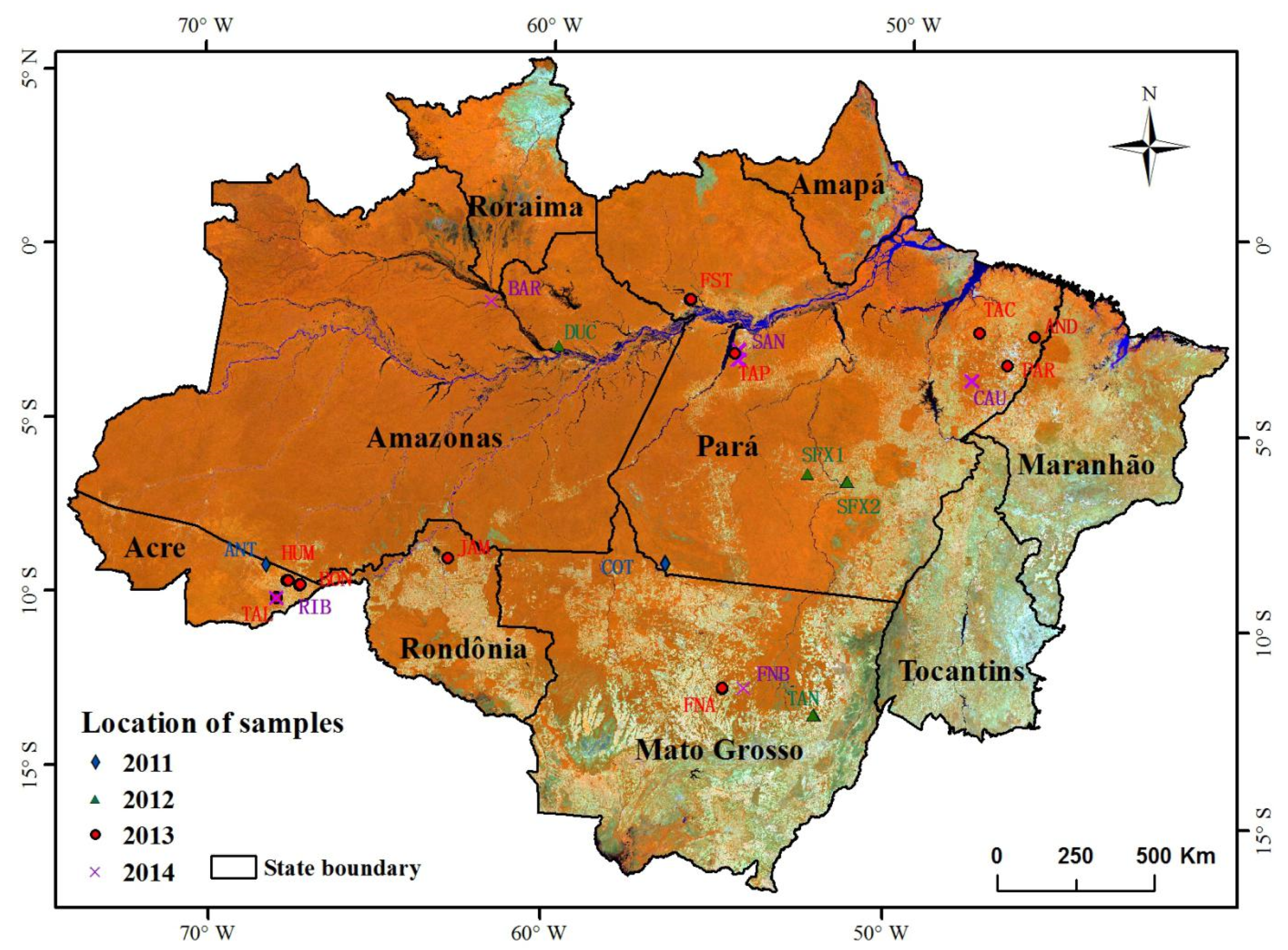
2.1. Study Area

The Brazilian Legal Amazon Region, which consists of the States of Roraima, Amapá, Amazonas, Pará, Acre, Rondônia, Mato Grosso, Tocantins, and part of Maranhão, was selected as our study area (Figure 1). It covers about 5.2 million km2 and occupies 59% of Brazil’s land area [57]. The region includes three biomes: Amazon, encompassing the largest contiguous area of tropical forests on Earth; Cerrado, the Brazilian savanna, which occupies portions of Mato Grosso and Maranhão, and all of Tocantins; and Pantanal, a seasonally flooded savanna in southwestern Mato Grosso [58]. The climate is characterized by year-round warm temperatures (averaging 25 °C, with less than 2 °C annual variation and 5–10 °C diurnal variation), with a rainy season between November and March and a dry season between May and September. April and October are transition months [59]. However, such an enormous region has different temperature and precipitation regimes, with the northern portion showing a significant heterogeneity in terms of the distribution of seasonal precipitation and southern and eastern portions showing a dry season of five months. Amazonian soils are divided into oxisols (45.5%), ultisols (29.4%), entisols (14.9%), alfisols (4.1%), inceptisols (3.3%), spodosols (2.2%), mollisols (0.8%), and vertisols (0.1%) [60].
Large-scale processes of colonization, deforestation, and forest degradation in the Brazilian Amazon began in the early 1970s, with settlement projects and construction of roads connecting the region with the southern and northeastern portions of the country. Since 1970, deforestation has resulted in more than 0.7 million km2 of forest loss [61]. There is a significant uncertainty about the amount and spatial distribution of forest aboveground biomass in the Brazilian Amazon, but it is generally above 300 Mg/ha in its central to western portions. Transitional forests in the southern portions of the region have biomass amounts ranging from 100 to 200 Mg/ha [48]. Forest degradation has affected the amount of AGB in Amazonian forests, which calls for cutting edge studies on this topic [5].

2.2. Datasets Used in This Research

In our research, we used two kinds of remotely sensed data, namely airborne LiDAR and MODIS data, as well as ancillary data (annual land cover maps, 2011–2017) (see Table 1). Airborne LiDAR data from 23 sites in five states—Acre, Rondônia, Mato Grosso, Pará, and Amazonas—were acquired for 2011–2014 and downloaded from the repository at Brazilian Agricultural Research Corporation [62]. Among the 23 sites, 18 were the same as those used by Longo et al. [5]. The spatial locations of all sites are illustrated in Figure 1. The airborne LiDAR data for 2011–2014 were acquired at an average of 850–900 m above ground by Geoid Laser Mapping, Ltd., using the ALTM (Airborne Laser Terrain Mapper) Orion M-200. We established a minimum return density of more than four points per square meter for data collection. A detailed description of the LiDAR systems used for surveys can be found in the paper by Longo et al. [5]. The downloaded point cloud data of each site were processed to generate a digital terrain model (DTM) and digital surface model (DSM) with a cell size of 1 × 1 m. The CHM data were obtained by subtracting DTM from DSM.
The MODIS spectral reflectance from nadir bidirectional distribution function (BRDF) adjusted reflectance (NBAR) data at a spatial resolution of 500 m (MCD43A4) was used to map the ACD distribution of the entire Legal Amazon region. Seven BRDF-corrected spectral bands—red (B1—Red; 620–670 nm), near-infrared (B2—NIR; 841–876 nm), blue (B3—Blue; 459–479 nm), green (B4—Green; 545–565 nm), middle infrared (B5—MIR; 1230–1250 nm), shortwave infrared 1 (B6—SWIR1; 1628–1652 nm), and shortwave infrared 2 (B7—SWIR2; 2105–2155 nm)—covering the study area between 2011 and 2017 were processed using the Google Earth Engine (GEE) platform. To minimize the impacts of clouds on MODIS imagery, a dataset of annually composited cloud-free images was produced by averaging the values from all images from a certain year for the pixels without clouds; that is, only the high-quality pixels in all seven bands were extracted.
The annual land cover maps were downloaded from the Brazilian Annual Land Use and Land Cover Mapping Project [63]. The land cover datasets at 30 × 30 m were developed from Landsat images using extensive machine learning algorithms through the GEE platform. The original land cover classification system consists of 21 land cover types under five broad categories: forest, non-forest natural formation, farming, non-vegetated, and water. The complete description of the project can be found at MapBiomas [63]. The land cover classification image was recoded as forest and others, then aggregated into a new dataset, where the pixel size changed from 30 × 30 m to 500 × 500 m using the majority algorithm, meaning the resampled annul forest image has the same cell size as MODIS data.

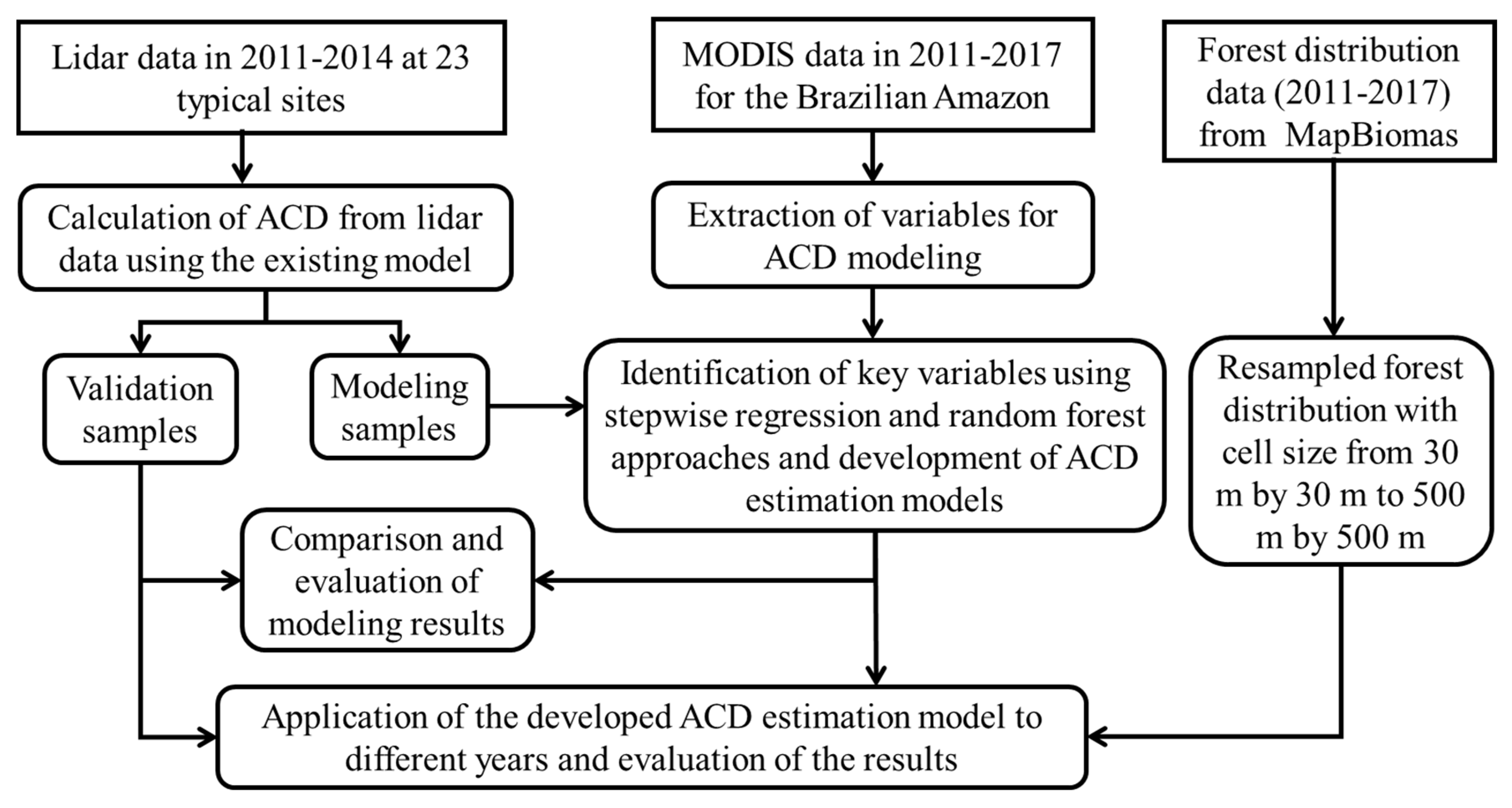
2.3. Strategy of This Research

The framework for mapping the ACD distribution is illustrated in Figure 2, including the following steps: (1) calculation of ACD for the LiDAR sites based on LiDAR metrics generated from LiDAR point data; (2) preparation of samples for modeling and validation, which are from the LiDAR-based ACD; (3) extraction and selection of variables from MODIS data; (4) establishment of ACD models based on linear regression (LR) and RF approaches; (5) prediction of ACD for entire study area using the developed model by incorporating the resampled forest image and evaluation of the prediction results.

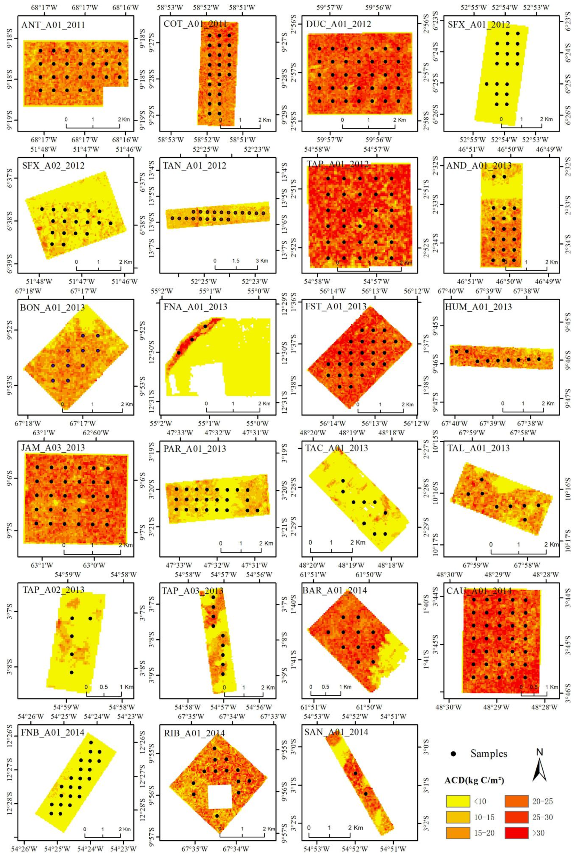
2.4. Calculation of Aboveground Carbon Density for the 23 Sites Using LiDAR Data

Longo et al. [5] developed a general ACD model based on airborne LiDAR metrics and ACD samples from 18 study sites, for which LiDAR metrics and ACD were calculated at a plot size of 50 × 50 m. The ACD model explained 70% of the variance across forest types. In our research, we applied this model to predict ACD distributions in the 23 sites. The ACD model is re-expressed as follows:
ACD = 0.20 h m 2.02   k h 0.66   h 5 0.11   h 10 0.32   h I Q 0.50   h 100 0.82
where ℎm is the average height; k is the kurtosis of the height distribution; ℎ5 and ℎ10 are the 5th and 10th percentile heights, respectively; ℎIQ is the interquartile range (h75h25); and ℎ100 is the maximum height. All of these variables were calculated based on the plot size of 50 × 50 m. The predicted ACD spatial distributions for 23 sites are illustrated in Figure 3, indicating considerably different ACD ranges among these sites.
The LiDAR-derived ACD images with a cell size of 50 × 50 m for all sites were aggregated to a cell size of 500 × 500 m using an averaging algorithm to match the MODIS data. The new ACD data were overlaid on the MODIS data for sample plot collection. A systematic sampling approach at one pixel interval (500 m) was used to collect initial samples for each site. These samples were refined by overlaying them on the forest map. The samples located at the borders of LiDAR sites and the non-forest areas were removed so that all selected samples for ACD modeling and validation were located in the forest regions. Finally, a total of 368 samples were collected. As shown in Figure 3, the numbers of samples from 23 sites are considerably different because of the sizes and shapes of LiDAR sites and the forest distributions. The statistical results for these samples are summarized in Table 2. Based on the statistical results, the ACD values are in the range of 0.3 to 31.6 kg C/m2, with a mean value of 19.1 kg C/m2 and standard deviation of 7.5 kg C/m2. However, the ACD ranges have considerably different values among the 23 sites. Some LiDAR sites, such as SFX_A01_2012, have ACD values of less than 10 kg C/m2, while other sites, such as CAU_A01_2014, have ACD values as high as over 30 kg C/m2 in some pixels. These different ACD ranges provide reasonably good distribution of the ACD samples. These samples were randomly separated into two groups: 60% of the samples were used for modeling and 40% for validation.

2.5. MODIS Potential Variable Predictors of ACD

One key step in the ACD modeling procedure is to extract suitable variables from MODIS data. Spectral bands and spectral indices are the most commonly used predictors [7]. Different types of spectral indices can be used as potential predictors. Most of them are from visible and NIR bands, such as the ratio vegetation index (RVI), NDVI, soil-adjusted vegetation index (SAVI), modified soil-adjusted vegetation index (MSAVI), and optimized soil-adjusted vegetation index (OSAVI). The SWIR spectral band is one of the most important variables in predicting AGB [64,65,66], and spectral indices containing SWIR have stronger relationships with AGB [67,68] under complex forest structures. Thus, some spectral indices derived from SWIR were also calculated. Table 3 lists the spectral indices used in this research and their calculation formulae. A total of 22 predictor variables were explored, including seven MODIS BRDF spectral bands and 15 spectral derivations.

2.6. Identification of Key Variables and Development of Aboveground Carbon Density Estimation Models

The relationships between ACD and MODIS-derived variables were examined using Pearson’s correlation analysis to understand the potential variables that can be used for ACD modeling. Because the selection of key variables is a critical step in modeling [6], we used stepwise regression and the RF approach to identify key variables. Stepwise regression may be the most commonly used approach to identify key variables for biomass estimation modeling, assuming linear relationships exist between biomass and independent variables [7]. However, in reality, this assumption may not be true. RF is an effective tool to rank the importance of independent variables; thus, we can identify key variables for developing estimation models without the linear relationship assumption. After determination of key variables, we used LR and RF to develop ACD estimation models.
The LR model can be expressed as:
y = b0 + b1×1 + b2×2 + ⋯ + bnxn + ε
where y is the ACD sample data from LiDAR-estimated ACD data; x1, x2, …, xn are prediction variables derived from MODIS data (spectral bands and spectral indices); b0 is a constant; b1, b2, …, bn are regression coefficients; ε is the error item; and n is the number of variables.
Although different machine learning algorithms, such as artificial neural network (ANN), support vector machine (SVM), and random forest (RF) [7] algorithms, can be used for ACD modeling, RF is one of the machine learning algorithms that can effectively handle the high-dimensional variables [80]. Compared to ANN and SVM, RF has advantages in dealing with noisy data in training datasets, using either discrete or continuous datasets, and requiring much less time for large dataset processing and algorithm parameter optimization [7]. Therefore, this research used the RF algorithm to develop the ACD estimation model. Many publications have described the RF theory [81,82], so we do not need to explain it in detail here. The “randomForest” package in R software was used in this research. Two critical parameters—number of decision trees (ntree) and number of variables used in each node (mtry)—needed to be optimized. The optimized ntree and mtry values were determined when the smallest root mean squared error (RMSE) was reached through iterative processes of adjusting mtry and ntree parameters based on training data. In general, mtry was selected as one-third of the number of variables, while ntree was within the range of 100–5000. Since RF can provide rank the variables by importance but does not describe the relationships between the variables, Pearson’s correlation analysis can be used to examine those relationships to remove some variables that have high correlations to one another. If the correlation coefficients between two variables had 0.85 or higher, one was dropped and RF was conducted again. The procedure was repeated until the minimum number of variables was achieved, while the RMSE remained stable. The RF algorithm based on the finally selected variables was used to predict ACD for the entire study area for 2011–2017. In total, 60% of the samples (see Table 2) were randomly selected to develop the ACD estimation models.

2.7. Evaluation of the Modeling Results

Considering the advantages of spectral indices over spectral bands in reducing environmental impacts, two data scenarios—spectral indices alone and a combination of spectral bands and indices—were examined for ACD modeling using LR and RF approaches, respectively. The modeling results from different data sources and modeling approaches were then quantitatively evaluated using the coefficient of determination (R2), RMSE, and relative RMSE (RMSEr) [7,83]. This research used all validation samples from the sites for all years between 2011 and 2014 for overall assessment; meanwhile, an evaluation was also conducted for individual prediction results from 2012, 2013, and 2014 using the available validation samples. In total, 40% of the samples were randomly selected for use as validation samples.

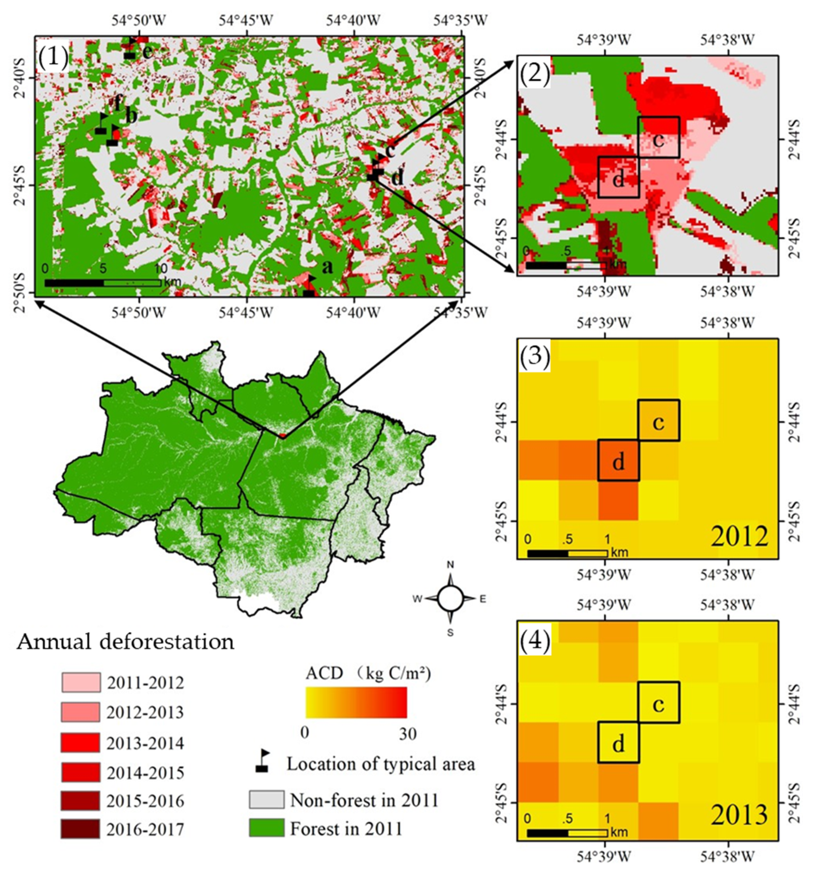
2.8. Impacts of Deforestation on Aboveground Carbon Dynamics

After developing the annual ACD distribution maps between 2011 and 2017 using the best ACD estimation model, we examined the annual ACD change and analyzed the impacts of forest disturbance on ACD dynamics. Considering the uncertainty in estimations, we mainly focused on the analysis of whether ACD change due to deforestation can be detected and how different deforestation rates can be reflected in the ACD change. The deforestation rate here is defined as the ratio of the number of deforested pixels to the total number of pixels within the window size of 17 × 17 pixels in Landsat-derived forest maps, corresponding to one cell in MODIS data. Therefore, based on the annual land use and land cover dataset developed from Landsat data for 2011–2017, we recoded these data as forest and non-forest and selected typical regions in which to identify deforestation sites with various rates. The deforested areas were linked to annual ACD estimation results to analyze the impacts of various deforestation rates on ACD estimates. The procedure to conduct this analysis is illustrated in Figure 4.

3. Results

3.1. Analysis of the Relationships between Aboveground Carbon Density and MODIS-Derived Variables

The correlation coefficients between ACD and MODIS variables (Table 4) indicate that individual spectral bands have significantly negative correlations with ACD, of which SWIR2 has the highest r value of −0.74, followed by red and SWIR1 bands, with r values of −0.65 and −0.63, respectively. The selected spectral indices also have significant correlation with ACD, either negative or positive. MD75 has the highest r value of −0.68, followed by NDII7 and albedo, with r values of 0.66 and −0.63, respectively. This result indicates that SWIR2 and spectral indices containing SWIR2 have higher correlations with ACD than other spectral bands or spectral indices, which is similar to results from previous studies based on Landsat imagery in the Brazilian Amazon [67].

3.2. Analysis of Aboveground Carbon Density Estimation Models

The best models using LR and RF based on spectral indices alone and combinations of spectral indices and spectral bands (Table 5) indicate the important roles of the red spectral band and the spectral indices containing SWIR2 in both LR and RF models. Considering R2 values, two data sources have similar performance, but the variables are slightly different, especially for the LR models. When spectral bands and indices were used together in the LR model, red and SWIR2 bands had more important roles than the spectral index based on beta values.

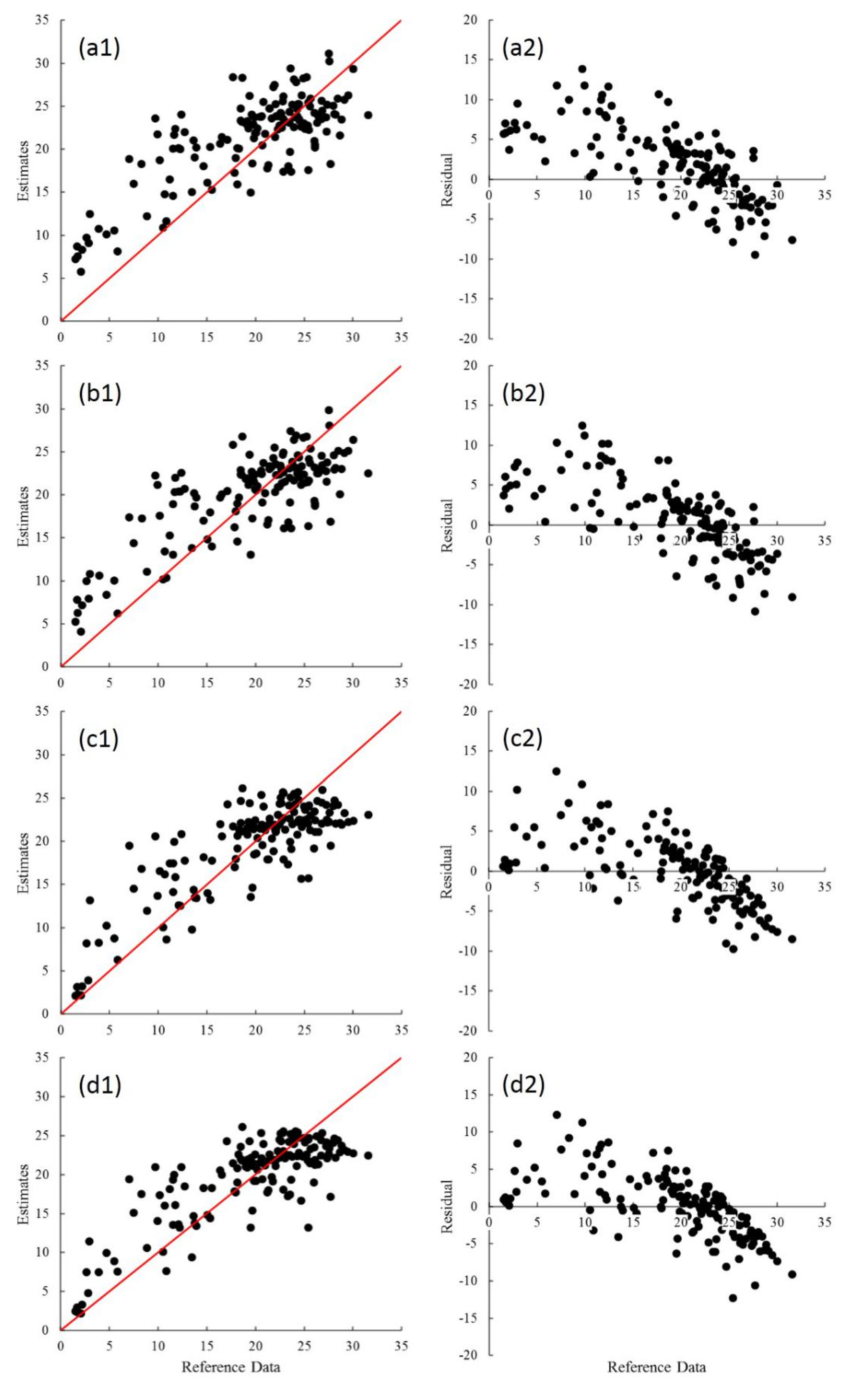
3.3. Comparative Analysis of Aboveground Carbon Density Prediction Results

Evaluation of the modeling results (Table 6) indicates that the combination of spectral indices and bands slightly improved the overall ACD estimation when LR was used but did not when using RF. Overall, the RF-based algorithm using spectral indices provided the best performance, with an R2 value of 0.67 and RMSE of 4.18 kg C/m2. When the developed models were used for ACD prediction for 2011–2017, the accuracy assessment results based on individual years from 2012 to 2014 indicate that the RF-based approach, using either spectral indices alone or a combination of spectral indices and bands, provides slightly better estimation results for 2012 and 2013 than the LR-based models do. However, the estimation performances were similar for LR and RF in the 2014 estimations.
The scatterplots and residuals (see Figure 5) show the similar performances of the LR and RF models based on either spectral indices or a combination of spectral indices and bands; that is, ACD estimates and reference data have linear relationships (Figure 5a1–d1). Overestimation and underestimation, which are obvious for each model, are different in the LR and RF modeling results (Figure 5a2–d2). For example, the overestimation is slightly better in RF-based modeling results compared to the LR-based estimation; this is especially obvious when the ACD is between 10 and 15 kg C/m2. The comparison of the two modeling results indicates that both methods have different advantages. For example, the LR is better in reducing the underestimation problem, especially when the ACD is greater than 25 kg C/m2, while RF is better in reducing overestimation. Figure 5 shows that the RF model has relatively less prediction ability than the LR model when the ACD is high, for example greater than 25 kg C/m2.
This analysis is based only on the overall performances of different modeling results with two data scenarios and two algorithms, and cannot determine the performances at different ACD ranges. As summarized in Table 7, the ACD modeling results show the highest RMSEr values of 116.8–158.7% when the ACD is less than 10 kg C/m2, implying poor performances of these models for ACD prediction within that range. In contrast, the ACD predictions have the lowest RMSE values of 2.57–2.89 kg C/m2 and lowest RMSEr values of 11.3–12.7% when the ACD is 20–25 kg C/m2, implying the good performance of each model in this range. Although RF based on spectral indices alone provided the best modeling performance, for ACD values greater than 25 kg C/m2, the LR model based on spectral indices alone provided better estimation than RF-based models, implying different effects of datasets and modeling algorithms on ACD estimations and a relationship between ACD ranges and performance.

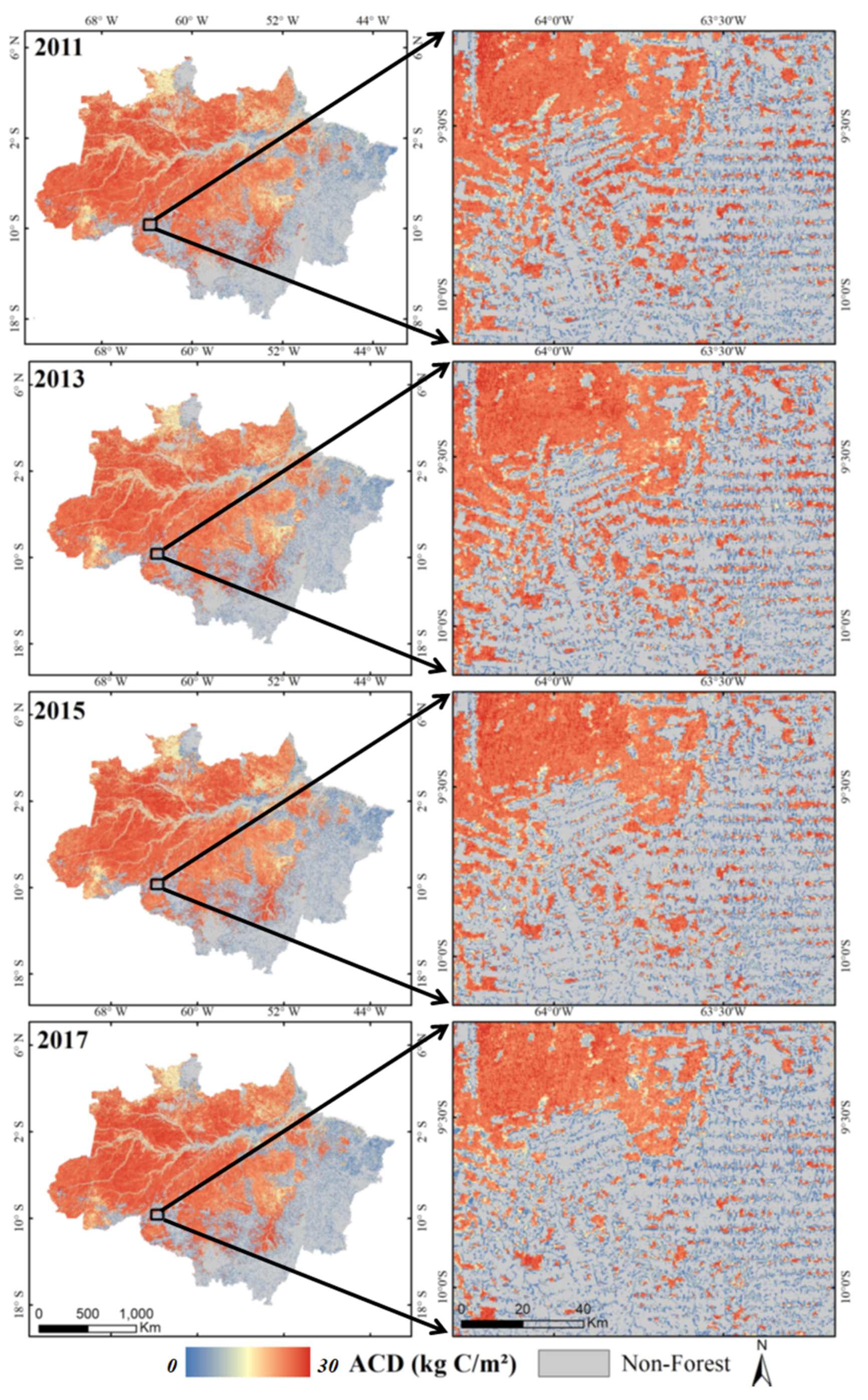
3.4. Spatial Distribution of Predicted Aboveground Carbon Density

Since the RF model based on spectral indices performed best, this model was used to predict the ACD distribution values for the entire study area in 2011 and 2017. As illustrated in Figure 6, all predicted ACD images have similar spatial patterns; that is, high ACD pixels were mainly distributed in the northern, western, and central parts, which were mainly over 20 kg C/m2, while low ACD pixels (<10 kg C/m2) were located in the southern and eastern parts due to deforestation. Comparison of the spatial patterns of ACD distributions indicates that the ACD values of many forested pixels in the northern area might be underestimated due to the cloud contamination problem, involving mixed pixels consisting of forest and clouds.

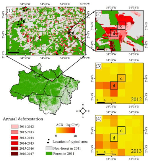
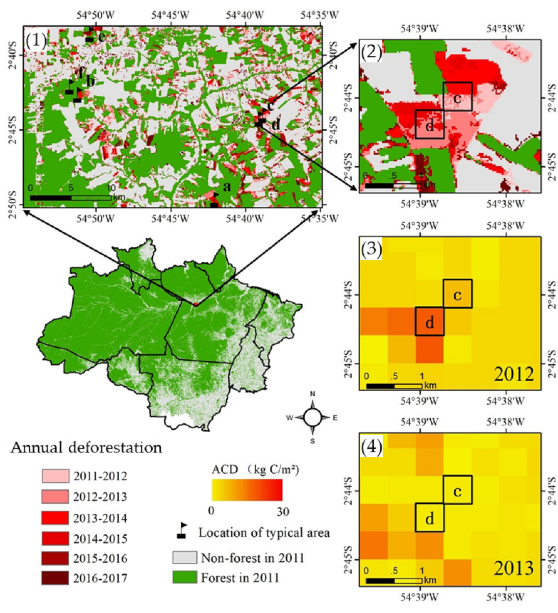
3.5. Aboveground Carbon Change Caused by Deforestation

In the Amazon basin, it is very important to know how much ACD could be lost due to deforestation, in addition to understanding whether the MODIS-derived ACD estimates can respond to different deforestation rates. As shown in Table 8, the ACD value dropped rapidly when the deforestation rate reached 44.9% (e.g., plot b) or higher (e.g., 56.3% in plot d and 58.2% in plot e). However, for low deforestation rates (e.g., 33.6% in plot f and 38.7% in plot e), the ACD values did not change significantly; that is, the amount of ACD change was less than the RMSE value. This situation implies that when the deforestation area is close to or more than one-half of the cell size of the MODIS pixel, such deforestation can be reflected by the significant drop over two successive years in the ACD estimates; however, when the deforestation size is small relative to a MODIS pixel, the ACD dynamics are not sensitive to such changes. As shown in plot f, the annual ACD estimates in 2012 and 2013 were 19.0 kg and 19.7 kg C/m2, respectively, although a small amount of deforestation (5.9%) occurred in this period; a similar case was found in plot d, where a deforestation rate of 33.6% occurred between 2011 and 2012, however the ACD only dropped by 0.2 kg C/m2 from 7.8 to 7.6 kg C/m2. Comprehensive analysis of Table 7 and Table 8 and the annual ACD maps (Figure 6) indicates that the annual ACD change cannot effectively respond to forest disturbance or growth due to the annual ACD change being less than the RMSE amount. For instance, when the ACD is less than 10 kg C/m2, the RMSE can be as high as 5.86 kg C/m2, or when the ACD is greater than 25 kg C/m2, the RMSE can be 5.10 kg C/m2 (Table 7). On the other hand, high deforestation rates indeed resulted in significant changes in ACD estimates, implying that the ACD estimates using MODIS data can be used to evaluate the ACD loss due to deforestation when the deforested area reaches one-half of the pixel size of MODIS data, i.e., 250 × 250 m.

4. Discussion

Various factors could cause uncertainties in the estimation of biomass or carbon stocks [23,49]. Such factors could be the ACD reference data calculated from field measurements using allometric equations; the big regional differences in mean wood density among different tree species; various disturbances such as wind blow-downs, droughts, and deforestation that influence forest species composition and structures; the variables used for ACD modeling; and the relevant algorithms [23,84]. However, some factors such as different wood density and disturbance are often ignored in large-scale estimation of the carbon budget [85,86] because of difficulties in quantifying their impacts on modeling effects. In this section, we mainly discuss the uncertainties caused by data saturation, mixed pixels, cloud contamination, overfitting problems, and selection of data sources and modeling algorithms. We also provide a brief discussion of the advantages and limitations of this study.

4.1. Overestimation and Underestimation Problems

In AGB estimation, overestimation and underestimation are common when using Landsat images; that is, overestimation when AGB is relatively small (e.g., less than 40 Mg/ha) and underestimation when AGB is relatively high (e.g., 150 Mg/ha) [87,88,89]. This research also confirmed that ACD estimation has similar problems to MODIS data—overestimation when ACD is less than 10 kg C/m2 and underestimation when ACD is greater than 25 kg C/m2, as shown in Figure 5. The saturation problem in MODIS data is also obvious, as shown in Figure 7, resulting in considerable ACD underestimation. Additionally, the coarse spatial resolution in MODIS data produced a serious mixed pixel problem, especially in the transition areas between forest and deforestation areas, resulting in considerable ACD overestimation. This situation implies the challenge of ACD estimation using MODIS data alone and indicates the necessity to incorporate other data sources in ACD modeling.
In addition to the data saturation and mixed pixel problems, the selection of a suitable modeling algorithm is also needed to reduce overestimation and underestimation problems. The machine learning algorithms often have an overfitting problem, resulting in high estimation uncertainty when the AGB is relatively high (e.g., greater than 120 Mg/ha) or low (e.g., less than 40 Mg/ha), as shown in subtropical AGB modeling using Landsat imagery [87,88]. This research on ACD estimation in a tropical region using MODIS data also confirmed this problem. The overfitting problem is common and cannot be completely eliminated, which is especially serious when the training sample is not large enough. When few samples are used, SVM may provide better modeling results than RF, but when a large number of samples are available, RF can reduce the overfitting problem through boosting and bagging technologies compared to other machine learning algorithms [7,88]. Therefore, it is important to increase the number of training samples. Airborne LiDAR data, especially when an unmanned vehicle is used, provide an important source of quickly and copiously collected samples for model development and validation. As shown in Figure 5, RF has a more serious underestimation problem than LR when ACD is relatively high, but has less of an overestimation problem than LR when ACD is relatively small, implying that modeling performance corresponds to ACD ranges. This situation indicates the need to conduct decision-level fusion based on the estimation results from different modeling approaches to improve estimation accuracy [90].

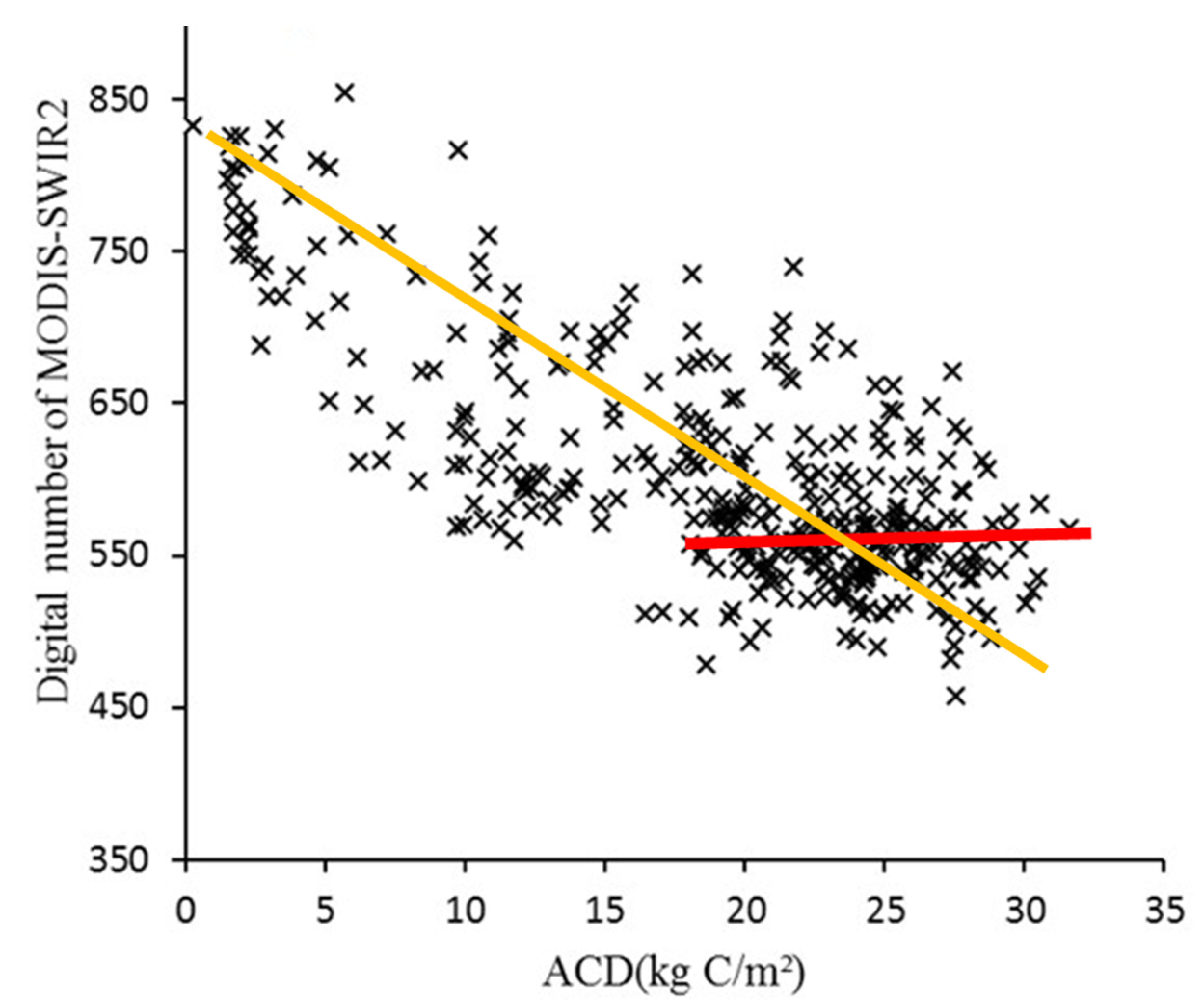
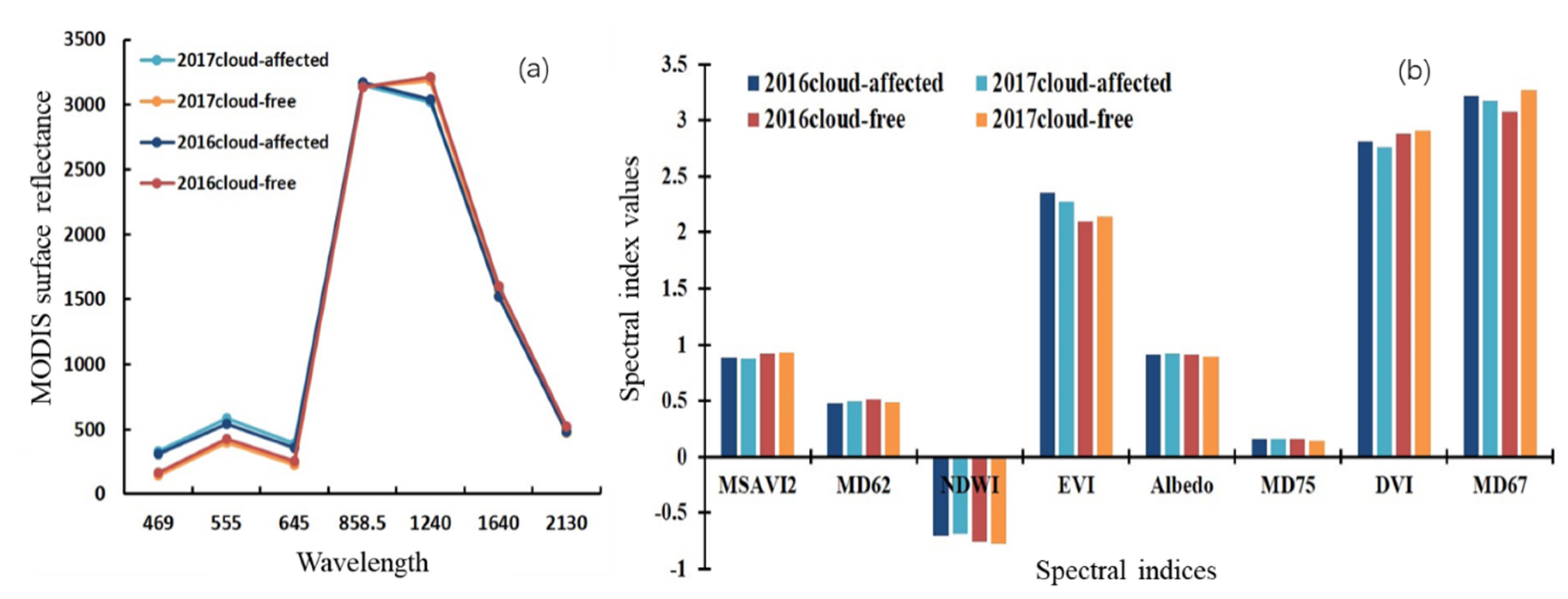
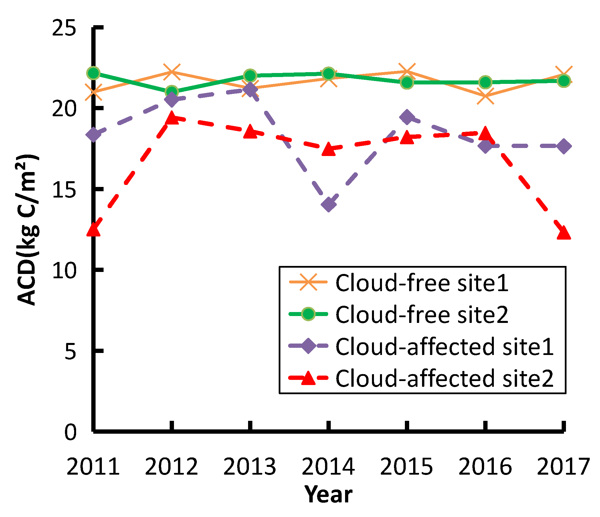
4.2. Impacts of Cloud Contamination on Modeling Performance

The variation of spectral signatures caused by environmental conditions can considerably influence modeling results, and thus lead to high estimation uncertainties when the model is applied to different years. As illustrated in Figure 8a, visible bands and MIR are seriously influenced by the cloud contamination problem; that is, the cloud-contaminated pixels have higher spectral signature values in MODIS visible bands than cloud-free pixels, while the inverse is true for MIR. The NIR, SWIR1, and SWIR2 bands are less influenced by the cloud problem. Because of the different impacts of cloud contamination on spectral signatures, the spectral indices are also influenced to various degrees, as shown in Figure 8b. This problem causes serious ACD underestimation, as shown in Figure 9. The pixels without effects from clouds have similar ACD annual estimations, implying the robustness of this RF-based model for ACD prediction; however, ACD was considerably underestimated in the pixels with cloud impacts. The ACD spatial distribution in Figure 6 confirmed this problem—forests in the north and northeast regions were prone to underestimation in different years due to frequent clouds, even using the yearly MODIS composite images. The cloud problem makes ACD estimation difficult when using optical sensor data, especially in the Amazon basin, which has frequent clouds all year.
In order to reduce the cloud contamination problem in the MODIS data, the use of satellite radar data such as ALOS PALSAR (Advanced Land Observing Satellite/Phased Array type L-band Synthetic Aperture Radar) L-band and Radarsat C-band data may be an alternative [91,92], however data saturation in these images cannot improve the ACD estimation performance [93]. The long-wavelength P-band radar data can reduce the data saturation problem and may be a promising data source for ACD estimation. However, only limited studies have explored the use of simulated P-band data [94]. More research is needed to examine ACD estimation when satellite radar P-band data are available in the near future.

4.3. Data Sources and Uncertainties

Various types of spaceborne and airborne sensor data are available, but most belong to optical sensor data. Landsat may be the most common data source for land cover mapping or biomass modeling [7]. However, in the Amazon region, cloud cover is a big problem, resulting in difficulty in collecting cloud-free optical sensor data because of the low revisit period of the Landsat satellite. Another problem with using Landsat images in a large area such as the Amazon basin is that Landsat images from different dates have differing spectral reflectance values due to the impacts of atmospheric conditions, thus resulting in difficulty developing a biomass or ACD model without sufficient sample plots for each scene of a Landsat image [6]. Use of synthetic aperture radar (SAR) data can avoid the atmospheric-induced image acquisition problem, but at present there are no SAR data for public use at no cost, except the ALOS-1 PALSAR data with 25 m spatial resolution between 2006 and 2011. The daily available MODIS multispectral data can reduce the impacts of cloud problems, and the relatively coarse spatial resolution of MODIS is suitable for large-area studies. Therefore, many previous studies used MODIS data to map biomass distribution in large areas [40,41,42,43].
Some previous studies explored the incorporation of ancillary data, such as digital elevation models and climate data, into MODIS to develop ACD models [42,46], however the poor relationships between ACD and ancillary data, the data quality, and the spatial resolutions among different data sources did not significantly improve ACD modeling performance. In particular, improper incorporation of climate data into remotely sensed data may introduce extra modeling uncertainty due to its very coarse spatial resolution and the data quality problem itself. Special caution should be taken in the selection of proper variables from multiple data sources and relevant modeling algorithms. As spaceborne LiDAR data such as ICESat-2 ATLAS and GEDI have improved quality, incorporation of these data into optical sensor data (e.g., Landsat, MODIS) may further improve ACD modeling performance [33,34,35,95]. More research is needed to explore the integration of multiple data sources and advanced modeling approaches such as deep learning [89,96].
Previous studies have already indicated that the quality of samples used for ACD or biomass modeling is the most important factor inducing high estimation uncertainty [23,84,96]. Most of the time, we cannot do much to improve the quality of reference data, except that we can carefully conduct field measurements of the parameters used for ACD calculation and select proper allometric equations to calculate ACD for specific trees. Therefore, the critical step is to identify proper variables from multiple data sources and modeling approaches to develop the ACD estimation model [7,89]. Through analysis of major factors influencing ACD modeling uncertainty, we can better design an ACD modeling procedure to optimize each step [7]. Therefore, more research is needed to identify major factors influencing ACD estimation uncertainty, although it will be a challenge to quantitatively specify the various contributors.

4.4. Implication and Limitation of MODIS-Based ACD Modeling

This research indicates that the RF-based model can estimate ACD annually when we use the selected MODIS-derived variables and that the spatial distribution patterns look reasonable (Figure 6). Additionally, the MODIS data have advantages in ACD modeling over Landsat images in tropical regions considering the cloud problem and data availability. However, the high uncertainty when ACD is relatively high or low make it difficult to conduct dynamic ACD analysis annually, because the ACD estimation uncertainty may be higher than the real ACD change caused by disturbance or growth between two years, as confirmed in Table 8.
Since time series of Landsat and MODIS data are available, some previous research has explored the possibility of incorporating time series features into forest biomass and ACD dynamics [10,97,98]. However, rarely have studies successfully implemented ACD dynamics, considering the current technological status and limitations of optical sensor data [99]. The key is to considerably reduce the estimation uncertainties so that the ACD estimation error is less than the annual ACD change caused by growth or disturbance.

5. Conclusions

This research explored the integration of MODIS and LiDAR data for mapping of the ACD spatial distribution in the Brazilian Amazon. A comparative analysis of ACD modeling results using LR and RF based on spectral indices alone and on the combination of spectral indices and spectral bands indicates that overall the RF model based on spectral indices alone provided the best ACD estimation performance, with an R2 of 0.67 and RMSE of 4.18 kg C/m2. However, both LR and RF have different advantages and disadvantages; RF has better estimation performance than LR when the ACD is relatively small, such as less than 15 kg C/m2, while LR has slightly better extrapolation ability than RF, especially when the ACD is greater than 25 kg C/m2. Cloud contamination and data saturation are the major factors resulting in ACD underestimation, while the mixed pixel problem due to coarse spatial resolution is the major factor resulting in overestimation. Overfitting is another factor resulting in ACD over- or underestimation problems. More research is needed to reduce these problems by incorporating other data sources, such as canopy height features from the ICESat-2 ATLAS and GEDI data and ancillary data such as DEM and climate information, as well as by increasing the number of samples for modeling, especially the number of samples for very small or very high ACD values. Use of LiDAR data, especially by extensively using unmanned aerial vehicles in the near future, is an effective way to considerably increase the number of samples for modeling and validation. Use of satellite radar P-band data in the near future will solve the cloud problem in the Amazon Basin and may play an important role in improving ACD estimation.

Author Contributions

Conceptualization, D.L. and E.M.; methodology, X.J., G.L., and D.L.; software, X.J., G.L., and D.L.; validation, X.J. and G.L.; formal analysis, X.J. and G.L.; investigation, X.J. and G.L.; resources, M.B. and X.J.; data curation, X.J., E.M., and M.B.; writing of original draft, X.J., G.L., and D.L.; review and editing, X.J., G.L., D.L., E.M., and M.B.; visualization, X.J. and G.L.; supervision, D.L. and E.M.; project administration, D.L. and E.M.; funding acquisition, E.M. All authors have read and agreed to the published version of the manuscript.

Funding

This study was supported by the National Science Foundation of the United States under the program for Innovations at the Nexus of Food, Energy, and Water Systems (INFEWS) (grant #1639115). The funding sources are not responsible for the views espoused herein; these are the responsibility of the authors.

Acknowledgments

The authors would like to thank Michael Keller for providing comments for revising this manuscript. The LiDAR data used in this research were acquired by the Sustainable Landscapes Brazil project supported by the Brazilian Agricultural Research Corporation (EMBRAPA), the US Forest Service, USAID, and the US Department of State.

Conflicts of Interest

The authors declare no conflict of interest.

References

  1. Kindermann, G.E.; McCallum, I.; Fritz, S.; Obersteiner, M. A global forest growing stock, biomass and carbon map based on FAO statistics. Silva Fenn. 2008, 42, 387–396. [Google Scholar] [CrossRef] [Green Version]
  2. Mitchard, E.T.A. The tropical forest carbon cycle and climate change. Nature 2018, 559, 527–534. [Google Scholar] [CrossRef]
  3. Da Silva Dias, A.; Maretti, C.; Lawrence, K.; Charity, S.; Oliveira, D. Deforestation fronts in the Amazon region: Current situation and future trends—A preliminary summary. In Proceedings of the La COP 20: Perspectivas Desde el Sur, WWF Living Amazon Initiative; Universidad Ruiz de Montoya, District of Pueblo Libre: Lima, Peru, 9 December 2014; pp. 1–18. [Google Scholar]
  4. Irfan, U. Brazil’s Amazon Rainforest Destruction Is at Its Highest Rate in More Than a Decade. 18 November 2019. Available online: https://www.vox.com/science-and-health/2019/11/18/20970604/amazon-rainforest-2019-brazil-burning-deforestation-bolsonaro (accessed on 20 July 2020).
  5. Longo, M.; Keller, M.; Maiza, N.; Leitold, V.; Pinagé, E.R.; Baccini, A.; Saatchi, S.; Nogueira, E.M.; Batistella, M.; Morton, D.C. Aboveground biomass variability across intact and degraded forests in the Brazilian Amazon. Glob. Biogeochem. Cycles Res. 2016, 30, 1639–1660. [Google Scholar] [CrossRef] [Green Version]
  6. Lu, D. The potential and challenge of remote sensing-based biomass estimation. Int. J. Remote Sens. 2006, 27, 1297–1328. [Google Scholar] [CrossRef]
  7. Lu, D.; Chen, Q.; Wang, G.; Liu, L.; Li, G.; Moran, E. A survey of remote sensing-based aboveground biomass estimation methods in forest ecosystems. Int. J. Digit. Earth 2016, 9, 63–105. [Google Scholar] [CrossRef]
  8. Ghasemi, N.; Sahebi, M.R.; Mohammadzadeh, A. A review on biomass estimation methods using synthetic aperture radar data. Int. J. Geomat. Geosci. 2011, 1, 776–788. [Google Scholar]
  9. Wulder, M.A.; White, J.C.; Nelson, R.F.; Næsset, E.; Ørka, H.O.; Coops, N.C.; Hilker, T.; Bater, C.W.; Gobakken, T. Lidar sampling for large-area forest characterization: A review. Remote Sens. Environ. 2012, 121, 196–209. [Google Scholar] [CrossRef] [Green Version]
  10. Nguyen, T.H.; Jones, S.D.; Soto-Berelov, M.; Haywood, A.; Hislop, S. Monitoring aboveground forest biomass dynamics over three decades using Landsat time-series and single-date inventory data. Int. J. Appl. Earth Obs. Geoinf. 2020, 84, 101952. [Google Scholar] [CrossRef]
  11. Lefsky, M.A.; Cohen, W.B.; Harding, D.J.; Parker, G.G.; Acker, S.A.; Gower, S.T. Lidar remote sensing of above-ground biomass in three biomes. Glob. Ecol. Biogeogr. 2002, 11, 393–399. [Google Scholar] [CrossRef] [Green Version]
  12. Clark, M.L.; Roberts, D.A.; Ewel, J.J.; Clark, D.B. Estimation of tropical rain forest aboveground biomass with small-footprint lidar and hyperspectral sensors. Remote Sens. Environ. 2011, 115, 2931–2942. [Google Scholar] [CrossRef]
  13. Badreldin, N.; Sanchez-Azofeifa, A. Estimating forest biomass dynamics by integrating multi-temporal Landsat satellite images with ground and airborne LiDAR data in the Coal Valley Mine, Alberta, Canada. Remote Sens. 2015, 7, 2832–2849. [Google Scholar] [CrossRef] [Green Version]
  14. Drake, J.B.; Dubayah, R.O.; Clark, D.B.; Knox, R.G.; Blair, J.B.; Hofton, M.A.; Chazdon, R.L.; Weishampel, J.F.; Prince, S. Estimation of tropical forest structural characteristics using large-footprint lidar. Remote Sens. Environ. 2002, 79, 305–319. [Google Scholar] [CrossRef]
  15. Gleason, C.J.; Im, J. Forest biomass estimation from airborne LiDAR data using machine learning approaches. Remote Sens. Environ. 2012, 125, 80–91. [Google Scholar] [CrossRef]
  16. Baccini, A.; Asner, G.P. Improving pantropical forest carbon maps with airborne LiDAR sampling. Carbon Manag. 2013, 4, 591–600. [Google Scholar] [CrossRef] [Green Version]
  17. Chen, Q. LiDAR remote sensing of vegetation biomass. In Remote Sensing of Natural Resources; Wang, G., Weng, Q., Eds.; Taylor & Francis Group: Oxfordshire, UK, 2013; pp. 399–420. [Google Scholar]
  18. Zolkos, S.G.; Goetz, S.J.; Dubayah, R. A meta-analysis of terrestrial aboveground biomass estimation using lidar remote sensing. Remote Sens. Environ. 2013, 128, 289–298. [Google Scholar] [CrossRef]
  19. Chen, Q.; Vaglio Laurin, G.; Battles, J.J.; Saah, D. Integration of airborne lidar and vegetation types derived from aerial photography for mapping aboveground live biomass. Remote Sens. Environ. 2012, 121, 108–117. [Google Scholar] [CrossRef]
  20. Mongus, D.; Žalik, B. An efficient approach to 3D single tree-crown delineation in LiDAR data. ISPRS J. Photogramm. Remote Sens. 2015, 108, 219–233. [Google Scholar] [CrossRef]
  21. Wulder, M.A.; Coops, N.C.; Hudak, A.T.; Morsdorf, F.; Nelson, R.; Newnham, G.; Vastaranta, M. Status and prospects for LiDAR remote sensing of forested ecosystems. Can. J. Remote Sens. 2013, 39, 81–85. [Google Scholar] [CrossRef] [Green Version]
  22. Næsset, E. Area-based inventory in Norway—From innovation to an operational reality. In Forestry Applications of Airborne Laser Scanning: Concepts and Case Studies; Maltamo, M., Næssset, E., Vauhkonen, J., Eds.; Springer: Dordrecht, The Netherlands, 2014; pp. 218–240. [Google Scholar]
  23. Lu, D.; Chen, Q.; Wang, G.; Moran, E.; Batistella, M.; Zhang, M.; Vaglio Laurin, G.; Saah, D. Aboveground forest biomass estimation with Landsat and LiDAR data and uncertainty analysis of the estimates. Int. J. For. Res. 2012, 2012, 436537. [Google Scholar] [CrossRef]
  24. Lim, K.; Treitz, P.; Wulder, M.; St-Ongé, B.; Flood, M. LiDAR remote sensing of forest structure. Prog. Phys. Geogr. 2003, 27, 88–106. [Google Scholar] [CrossRef] [Green Version]
  25. Koch, B. Status and future of laser scanning, synthetic aperture radar and hyperspectral remote sensing data for forest biomass assessment. ISPRS J. Photogramm. Remote Sens. 2010, 65, 581–590. [Google Scholar] [CrossRef]
  26. Van Leeuwen, M.; Nieuwenhuis, M. Retrieval of forest structural parameters using LiDAR remote sensing. Eur. J. For. Res. 2010, 129, 749–770. [Google Scholar] [CrossRef]
  27. Gleason, C.; Im, J. A review of remote sensing of forest biomass and biofuel: Options for small-area applications. GIScience Remote Sens. 2011, 48, 141–170. [Google Scholar] [CrossRef]
  28. Lefsky, M.A.; Harding, D.J.; Keller, M.; Cohen, W.B.; Carabajal, C.C.; Del Bom Espirito-Santo, F.; Hunter, M.O.; de Oliveira, R. Estimates of forest canopy height and aboveground biomass using ICESat. Geophys. Res. Lett. 2005, 32, L22S02. [Google Scholar] [CrossRef] [Green Version]
  29. García, M.; Popescu, S.; Riaño, D.; Zhao, K.; Neuenschwander, A.; Agca, M.; Chuvieco, E. Characterization of canopy fuels using ICESat / GLAS data. Remote Sens. Environ. 2012, 123, 81–89. [Google Scholar] [CrossRef]
  30. Zwally, H.J.; Schutz, B.; Abdalati, W.; Abshire, J.; Bentley, C.; Brenner, A.; Bufton, J.; Dezio, J.; Hancock, D.; Harding, D.; et al. ICESat’s laser measurements of polar ice, atmosphere, ocean, and land. J. Geodyn. 2002, 34, 405–445. [Google Scholar] [CrossRef] [Green Version]
  31. Saarela, S.; Holm, S.; Healey, S.P.; Andersen, H.E.; Petersson, H.; Prentius, W.; Patterson, P.L.; Næsset, E.; Gregoire, T.G.; Ståhl, G. Generalized hierarchical model-based estimation for aboveground biomass assessment using GEDI and Landsat data. Remote Sens. 2018, 10, 1832. [Google Scholar] [CrossRef] [Green Version]
  32. Qi, W.; Saarela, S.; Armston, J.; Ståhl, G.; Dubayah, R. Forest biomass estimation over three distinct forest types using TanDEM-X InSAR data and simulated GEDI lidar data. Remote Sens. Environ. 2019, 232, 111283. [Google Scholar] [CrossRef]
  33. Narine, L.L.; Popescu, S.; Zhou, T.; Srinivasan, S.; Harbeck, K. Mapping forest aboveground biomass with a simulated ICESat-2 vegetation canopy product and Landsat data. Ann. For. Res. 2019, 62, 69–86. [Google Scholar] [CrossRef]
  34. Narine, L.L.; Popescu, S.C.; Malambo, L. Synergy of ICESat-2 and Landsat for mapping forest aboveground biomass with deep learning. Remote Sens. 2019, 11, 1503. [Google Scholar] [CrossRef]
  35. Narine, L.L.; Popescu, S.; Neuenschwander, A.; Zhou, T.; Srinivasan, S.; Harbeck, K. Estimating aboveground biomass and forest canopy cover with simulated ICESat-2 data. Remote Sens. Environ. 2019, 224, 1–11. [Google Scholar] [CrossRef]
  36. Barbosa, P.M.; Stroppiana, D.; Grégoire, J.-M.; Cardoso Pereira, J.M. An assessment of vegetation fire in Africa (1981–1991): Burned areas, burned biomass, and atmospheric emissions. Glob. Biogeochem. Cycles 1999, 13, 933–950. [Google Scholar] [CrossRef]
  37. Dong, J.; Kaufmann, R.K.; Myneni, R.B.; Tucker, C.J.; Kauppi, P.E.; Liski, J.; Buermann, W.; Alexeyev, V.; Hughes, M.K. Remote sensing estimates of boreal and temperate forest woody biomass: Carbon pools, sources, and sinks. Remote Sens. Environ. 2003, 84, 393–410. [Google Scholar] [CrossRef] [Green Version]
  38. Fensholt, R.; Sandholt, I.; Rasmussen, M.S.; Stisen, S.; Diouf, A. Evaluation of satellite based primary production modelling in the semi-arid Sahel. Remote Sens. Environ. 2006, 105, 173–188. [Google Scholar] [CrossRef]
  39. Asner, G.P.; Levick, S.R.; Smit, I.P.J. Remote sensing of fractional cover and biochemistry in Savannas. In Ecosystem Function in Savannas: Measurement and Modeling at Landscape to Global Scales; Hill, M.J., Hanan, N.P., Eds.; CRC Press: Boca Raton, FL, USA, 2010; pp. 195–217. [Google Scholar]
  40. Gallaun, H.; Zanchi, G.; Nabuurs, G.; Hengeveld, G.; Schardt, M.; Verkerk, P.J. EU-wide maps of growing stock and above-ground biomass in forests based on remote sensing and field measurements. For. Ecol. Manag. 2010, 260, 252–261. [Google Scholar] [CrossRef]
  41. Baccini, A.; Laporte, N.; Goetz, S.J.; Sun, M.; Dong, H. A first map of tropical Africa’s above-ground biomass derived from satellite imagery. Environ. Res. Lett. 2008, 3, 0450011. [Google Scholar] [CrossRef] [Green Version]
  42. Blackard, J.A.; Finco, M.V.; Helmer, E.H.; Holden, G.R.; Hoppus, M.L.; Jacobs, D.M.; Lister, A.J.; Moisen, G.G.; Nelson, M.D.; Riemann, R.; et al. Mapping U.S. forest biomass using nationwide forest inventory data and moderate resolution information. Remote Sens. Environ. 2008, 112, 1658–1677. [Google Scholar] [CrossRef]
  43. Beaudoin, A.; Bernier, P.Y.; Guindon, L.; Villemaire, P.; Guo, X.J.; Stinson, G.; Bergeron, T.; Magnussen, S.; Hall, R.J. Mapping attributes of Canada’s forests at moderate resolution through KNN and MODIS imagery. Can. J. For. Res. 2014, 44, 521–532. [Google Scholar] [CrossRef] [Green Version]
  44. Saatchi, S.S.; Harris, N.L.; Brown, S.; Lefsky, M.; Mitchard, E.T.A.; Salas, W.; Zutta, B.R.; Buermann, W.; Lewis, S.L.; Hagen, S.; et al. Benchmark map of forest carbon stocks in tropical regions across three continents. Proc. Natl. Acad. Sci. USA 2011, 108, 9899–9904. [Google Scholar] [CrossRef] [Green Version]
  45. Baccini, A.; Goetz, S.J.; Walker, W.S.; Laporte, N.T.; Sun, M.; Hackler, J.; Beck, P.S.A.A.; Dubayah, R.; Friedl, M.A.; Samanta, S.; et al. Estimated carbon dioxide emissions from tropical deforestation improved by carbon-density maps. Nat. Clim. Chang. 2012, 2, 182–185. [Google Scholar] [CrossRef]
  46. Hu, T.; Su, Y.; Xue, B.; Liu, J.; Zhao, X.; Fang, J.; Guo, Q. Mapping global forest aboveground biomass with spaceborne LiDAR, optical imagery, and forest inventory data. Remote Sens. 2016, 8, 565. [Google Scholar] [CrossRef] [Green Version]
  47. Chi, H.; Sun, G.; Huang, J.; Guo, Z.; Ni, W.; Fu, A. National forest aboveground biomass mapping from ICESat/GLAS Data and MODIS imagery in China. Remote Sens. 2015, 7, 5534–5564. [Google Scholar] [CrossRef] [Green Version]
  48. Saatchi, S.; Houghton, R.A.; Dos Santos Alvalá, R.C.; Soares, J.V.; Yu, Y.; Hole, W. Distribution of aboveground live biomass in the Amazon basin. Glob. Chang. Biol. 2007, 13, 816–837. [Google Scholar] [CrossRef]
  49. Mitchard, E.T.A.; Feldpausch, T.R.; Brienen, R.J.W.; Lopez-Gonzalez, G.; Monteagudo, A.; Baker, T.R.; Lewis, S.L.; Lloyd, J.; Quesada, C.A.; Gloor, M.; et al. Markedly divergent estimates of Amazon forest carbon density from ground plots and satellites. Glob. Ecol. Biogeogr. 2014, 23, 935–946. [Google Scholar] [CrossRef] [PubMed]
  50. Ometto, J.P.; Aguiar, A.P.; Assis, T.; Soler, L.; Valle, P.; Tejada, G.; Lapola, D.M.; Meir, P. Amazon forest biomass density maps: Tackling the uncertainty in carbon emission estimates. Clim. Chang. 2014, 124, 545–560. [Google Scholar] [CrossRef]
  51. Kumar, L.; Sinha, P.; Taylor, S.; Alqurashi, A.F. Review of the use of remote sensing for biomass estimation to support renewable energy generation. J. Appl. Remote Sens. 2015, 9, 097696. [Google Scholar] [CrossRef]
  52. Chave, J.; Davies, S.J.; Phillips, O.L.; Lewis, S.L.; Sist, P.; Schepaschenko, D.; Armston, J.; Baker, T.R.; Coomes, D.; Disney, M.; et al. Ground data are essential for biomass remote sensing missions. Surv. Geophys. 2019, 40, 863–880. [Google Scholar] [CrossRef]
  53. Marvin, D.C.; Asner, G.P.; Knapp, D.E.; Anderson, C.B.; Martin, R.E.; Sinca, F.; Tupayachi, R. Amazonian landscapes and the bias in field studies of forest structure and biomass. Proc. Natl. Acad. Sci. USA 2014, 111, E5224–E5232. [Google Scholar] [CrossRef] [Green Version]
  54. Wagner, F.; Rutishauser, E.; Blanc, L.; Herault, B. Effects of plot size and census interval on descriptors of forest structure and dynamics. Biotropica 2010, 42, 664–671. [Google Scholar] [CrossRef]
  55. Yan, E.; Lin, H.; Wang, G.; Sun, H. Multi-resolution mapping and accuracy assessment of forest carbon density by combining image and plot data from a nested and clustering sampling design. Remote Sens. 2016, 8, 571. [Google Scholar] [CrossRef] [Green Version]
  56. Li, L.; Guo, Q.; Tao, S.; Kelly, M.; Xu, G. Lidar with multi-temporal MODIS provide a means to upscale predictions of forest biomass. ISPRS J. Photogramm. Remote Sens. 2015, 102, 198–208. [Google Scholar] [CrossRef]
  57. de Almeida, C.A.; Coutinho, A.C.; Esquerdo, J.C.d.M.; Adami, M.; Venturieri, A.; Diniz, C.G.; Dessay, N.; Durieux, L.; Gomes, A.R. High spatial resolution land use and land cover mapping of the Brazilian legal Amazon in 2008 using Landsat-5/TM and MODIS data. Acta Amaz. 2016, 46, 291–302. [Google Scholar] [CrossRef]
  58. Tyukavina, A.; Hansen, M.C.; Potapov, P.V.; Stehman, S.V.; Smith-Rodriguez, K.; Okpa, C.; Aguilar, R. Types and rates of forest disturbance in Brazilian Legal Amazon, 2000–2013. Sci. Adv. 2017. [Google Scholar] [CrossRef] [Green Version]
  59. Fisch, G.; Marengo, J.A.; Nobre, C.A. Uma revisão geral sobre o clima da Amazônia. Acta Amaz. 1998, 28, 101–126. [Google Scholar] [CrossRef]
  60. Cochrane, T.T.; Sánchez, P.A. Land resources, soils and their management in the Amazon region: A state of knowledge report. In Proceedings of the International Conference on Amazonian, Agriculture and Land-use Research, Cali, Colombia, April 16–18, 1980; CIAT Series 03E-3; Hecht, S.B., Ed.; Centro International de Agriculture Tropical: Cali, Colombia, 1982. [Google Scholar]
  61. Souza, C.M.Z.; Shimbo, J.; Rosa, M.R.; Parente, L.L.A.; Alencar, A.; Rudorff, B.F.T.; Hasenack, H.; Matsumoto, M.G.; Ferreira, L.; Souza-Filho, P.W.M.; et al. Reconstructing three decades of land use and land cover changes in Brazilian biomes with Landsat archive and Earth Engine. Remote Sens. 2020, 12, 2735. [Google Scholar] [CrossRef]
  62. dos-Santos, M.N.; Keller, M.M.; Morton, D.C. LiDAR Surveys Over Selected Forest Research Sites, Brazilian Amazon 2008–2018; ORNL DAAC: Oak Ridge, TN, USA, 2019. [Google Scholar]
  63. MapBiomas Project—Collection, V.4.1 of Brazilian Land Cover & Land Use Map Series. Available online: https://mapbiomas.org/en/project (accessed on 8 September 2020).
  64. López-Serrano, P.M.; Domínguez, J.L.C.; Corral-Rivas, J.J.; Jiménez, E.; López-Sánchez, C.A.; Vega-Nieva, D.J. Modeling of aboveground biomass with Landsat 8 OLI and machine learning in temperate forests. Forests 2020, 11, 11. [Google Scholar] [CrossRef] [Green Version]
  65. López-Serrano, P.M.; López-Sánchez, C.A.; Álvarez-González, J.G.; García-Gutiérrez, J. A comparison of machine learning techniques applied to Landsat-5 TM spectral data for biomass estimation. Can. J. Remote Sens. 2016, 42, 690–705. [Google Scholar] [CrossRef]
  66. López-Serrano, P.M.; Corral-Rivas, J.J.; Díaz-Varela, R.A.; Álvarez-González, J.G.; López-Sánchez, C.A. Evaluation of radiometric and atmospheric correction algorithms for aboveground forest biomass estimation using Landsat 5 TM data. Remote Sens. 2016, 8, 369. [Google Scholar] [CrossRef] [Green Version]
  67. Lu, D.; Mausel, P.; Brondízio, E.; Moran, E. Relationships between forest stand parameters and Landsat TM spectral responses in the Brazilian Amazon Basin. For. Ecol. Manag. 2004, 198, 149–167. [Google Scholar] [CrossRef]
  68. Freitas, S.R.; Mello, M.C.S.; Cruz, C.B.M. Relationships between forest structure and vegetation indices in Atlantic Rainforest. For. Ecol. Manag. 2005, 218, 353–362. [Google Scholar] [CrossRef]
  69. Rouse, J.W.; Haas, R.H.; Schell, J.A.; Deering, D.W. Monitoring the Vernal Advancement and Retrogradation (Green Wave Effect) of Natural Vegetation; Goddard Space Flight Center: Greenbelt, MD, USA, 1973. [Google Scholar]
  70. Richardson, A.J.; Wiegand, C.L. Distinguishing vegetation from soil background information. Photogramm. Eng. Remote Sens. 1977, 43, 1541–1552. [Google Scholar]
  71. Huete, A.; Didan, K.; Miura, T.; Rodriguez, E.P.; Gao, X.; Ferreira, L.G. Overview of the radiometric and biophysical performance of the MODIS vegetation indices. Remote Sens. Environ. 2002, 83, 195–213. [Google Scholar] [CrossRef]
  72. Tucker, C.J.; Sellers, P.J. Satellite remote sensing of primary production. Int. J. Remote Sens. 1986, 7, 1395–1416. [Google Scholar] [CrossRef]
  73. Huete, A.R. A soil-adjusted vegetation index (SAVI). Remote Sens. Environ. 1988, 25, 295–309. [Google Scholar] [CrossRef]
  74. Qi, J.; Chehbouni, A.; Huete, A.R.; Kerr, Y.H.; Sorooshian, S. A modified soil adjusted vegetation index. Remote Sens. Environ. 1994, 48, 119–126. [Google Scholar] [CrossRef]
  75. Rondeaux, G.; Steven, M.; Baret, F. Optimization of soil-adjusted vegetation indices. Remote Sens. Environ. 1996, 55, 95–107. [Google Scholar] [CrossRef]
  76. Gao, B.C. NDWI—A normalized difference water index for remote sensing of vegetation liquid water from space. Remote Sens. Environ. 1996, 58, 257–266. [Google Scholar] [CrossRef]
  77. Xiao, X.; Boles, S.; Liu, J.; Zhuang, D.; Frolking, S.; Li, C.; Salas, W.; Moore, B. Mapping paddy rice agriculture in southern China using multi-temporal MODIS images. Remote Sens. Environ. 2005, 95, 480–492. [Google Scholar] [CrossRef]
  78. Miller, J.D.; Thode, A.E. Quantifying burn severity in a heterogeneous landscape with a relative version of the delta Normalized Burn Ratio (dNBR). Remote Sens. Environ. 2007, 109, 66–80. [Google Scholar] [CrossRef]
  79. Dogan, H.M. Mineral composite assessment of Kelkit River Basin in Turkey by means of remote sensing. J. Earth Syst. Sci. 2009, 118, 701–710. [Google Scholar] [CrossRef]
  80. Breiman, L. Random forests. Mach. Learn. 2001, 45, 5–32. [Google Scholar] [CrossRef] [Green Version]
  81. Rodriguez-Galiano, V.F.; Ghimire, B.; Rogan, J.; Chica-Olmo, M.; Rigol-Sanchez, J.P. An assessment of the effectiveness of a random forest classifier for land-cover classification. ISPRS J. Photogramm. Remote Sens. 2012, 67, 93–104. [Google Scholar] [CrossRef]
  82. Belgiu, M.; Drăgu, L. Random forest in remote sensing: A review of applications and future directions. ISPRS J. Photogramm. Remote Sens. 2016, 114, 24–31. [Google Scholar] [CrossRef]
  83. Chen, Y.; Li, L.; Lu, D.; Li, D. Exploring bamboo forest aboveground biomass estimation using Sentinel-2 data. Remote Sens. 2019, 11, 7. [Google Scholar] [CrossRef] [Green Version]
  84. Chen, Q.; Vaglio Laurin, G.; Valentini, R. Uncertainty of remotely sensed aboveground biomass over an African tropical forest: Propagating errors from trees to plots to pixels. Remote Sens. Environ. 2015, 160, 134–143. [Google Scholar] [CrossRef]
  85. Houghton, R.A. Aboveground forest biomass and the global carbon balance. Glob. Chang. Biol. 2005, 11, 945–958. [Google Scholar] [CrossRef]
  86. Rödig, E.; Cuntz, M.; Rammig, A.; Fischer, R.; Taubert, F.; Huth, A. The importance of forest structure for carbon fluxes of the Amazon rainforest. Environ. Res. Lett. 2018, 13. [Google Scholar] [CrossRef]
  87. Zhao, P.; Lu, D.; Wang, G.; Wu, C.; Huang, Y.; Yu, S. Examining spectral reflectance saturation in Landsat imagery and corresponding solutions to improve forest aboveground biomass estimation. Remote Sens. 2016, 8, 469. [Google Scholar] [CrossRef] [Green Version]
  88. Gao, Y.; Lu, D.; Li, G.; Wang, G.; Chen, Q.; Liu, L.; Li, D. Comparative analysis of modeling algorithms for forest aboveground biomass estimation in a subtropical region. Remote Sens. 2018, 10, 627. [Google Scholar] [CrossRef] [Green Version]
  89. Rodríguez-Veiga, P.; Quegan, S.; Carreiras, J.; Persson, H.J.; Fransson, J.E.S.; Hoscilo, A.; Ziółkowski, D.; Stereńczak, K.; Lohberger, S.; Stängel, M.; et al. Forest biomass retrieval approaches from earth observation in different biomes. Int. J. Appl. Earth Obs. Geoinf. 2019, 77, 53–68. [Google Scholar] [CrossRef]
  90. Jiang, X.; Li, G.; Lu, D.; Chen, E.; Wei, X. Stratification-based forest aboveground biomass estimation in a subtropical region using airborne lidar data. Remote Sens. 2020, 12, 1101. [Google Scholar] [CrossRef] [Green Version]
  91. Santoro, M.; Cartus, O.; Carvalhais, N.; Rozendaal, D.; Avitabilie, V.; Araza, A.; de Bruin, S.; Herold, M.; Quegan, S.; Rodríguez Veiga, P.; et al. The global forest above-ground biomass pool for 2010 estimated from high-resolution satellite observations. Earth Syst. Sci. Data Discuss. 2020. [Google Scholar] [CrossRef]
  92. Li, G.; Lu, D.; Moran, E.; Dutra, L.; Batistella, M. A comparative analysis of ALOS PALSAR L-band and RADARSAT-2 C-band data for land-cover classification in a tropical moist region. ISPRS J. Photogramm. Remote Sens. 2012, 70, 26–38. [Google Scholar] [CrossRef] [Green Version]
  93. Zhao, P.; Lu, D.; Wang, G.; Liu, L.; Li, D.; Zhu, J.; Yu, S. Forest aboveground biomass estimation in Zhejiang Province using the integration of Landsat TM and ALOS PALSAR data. Int. J. Appl. Earth Obs. Geoinf. 2016, 53, 1–15. [Google Scholar] [CrossRef]
  94. Liao, Z.; He, B.; Quan, X.; van Dijk, A.I.J.M.; Qiu, S.; Yin, C. Biomass estimation in dense tropical forest using multiple information from single-baseline P-band PolInSAR data. Remote Sens. Environ. 2019, 221, 489–507. [Google Scholar] [CrossRef]
  95. Qi, W.; Lee, S.K.; Hancock, S.; Luthcke, S.; Tang, H.; Armston, J.; Dubayah, R. Improved forest height estimation by fusion of simulated GEDI Lidar data and TanDEM-X InSAR data. Remote Sens. Environ. 2019, 221, 621–634. [Google Scholar] [CrossRef] [Green Version]
  96. Bispo, P.C.; Rodríguez-Veiga, P.; Zimbres, B.; do Couto de Miranda, S.; Giusti Cezare, C.H.; Fleming, S.; Baldacchino, F.; Louis, V.; Rains, D.; Garcia, M.; et al. Woody aboveground biomass mapping of the brazilian savanna with a multi-sensor and machine learning approach. Remote Sens. 2020, 12, 2685. [Google Scholar] [CrossRef]
  97. Baccini, A.; Walker, W.; Carvalho, L.; Farina, M.; Sulla-Menashe, D.; Houghton, R.A. Tropical forests are a net carbon source based on aboveground measurements of gain and loss. Science 2017, 358, 230–234. [Google Scholar] [CrossRef] [Green Version]
  98. Nguyen, T.H.; Jones, S.; Soto-Berelov, M.; Haywood, A.; Hislop, S. Landsat time-series for estimating forest aboveground biomass and its dynamics across space and time: A review. Remote Sens. 2020, 12, 98. [Google Scholar] [CrossRef] [Green Version]
  99. Hansen, M.C.; Potapov, P.; Tyukavina, A. Comment on “Tropical forests are a net carbon source based on aboveground measurements of gain and loss”. Science 2019, 363, eaar3629. [Google Scholar] [CrossRef] [Green Version]
Figure 1. The color composite of the 2017 moderate-resolution imaging spectroradiometer (MODIS) data showing the Amazon basin and light detection and ranging (LiDAR) data sites for different years.
Remotesensing 12 03330 g001
Figure 2. Strategy of mapping aboveground carbon density (ACD) distribution in the Brazilian Amazon basin using MODIS and LiDAR data.
Remotesensing 12 03330 g002
Figure 3. Spatial distribution of predicted aboveground carbon density (ACD) using airborne LiDAR data for 23 study sites in 2011–2014 and the selected samples for modeling and validation.
Remotesensing 12 03330 g003
Figure 4. The strategy of linking deforestation images to ACD estimates to examine the impacts of deforestation rates on ACD dynamics: (1) annual deforestation image compiled from Landsat images in 2011–2017; (2) two plots with a window size of 17 × 17 pixels showing deforestation rates; (3,4) ACD estimates in 2012 and 2013, respectively, using random forest based on spectral indices from the MODIS data.
Remotesensing 12 03330 g004
Figure 5. The relationships between forest aboveground carbon density (ACD) estimates and reference data: (a1,b1) linear regression models based on spectral indices alone and a combination of spectral indices and bands, respectively; (c1,d1) random forest models based on spectral indices and a combination of spectral indices and bands, respectively; (a2d2) residuals of ACD estimates against reference data corresponding to each estimation model.
Remotesensing 12 03330 g005
Figure 6. Spatial distribution of aboveground carbon density (ACD) estimation using the random forest approach for 2011–2017.
Remotesensing 12 03330 g006
Figure 7. The relationship between spectral values of SWIR2 and aboveground carbon density (ACD), showing the data saturation problem. The symbol "×" shows the samples used for establishing the relationships between ACD and the SWIR2 band; yellow line shows the negative linear trend, that is, the SWIR2 values decrease as ACD values increase; red line shows that even ACD values increase, SWIR2 values do not show obvious change, meaning the data saturation problem in the MODIS data.
Remotesensing 12 03330 g007
Figure 8. The impacts of cloud contamination on (a) spectral signatures and (b) spectral indices from the 2016 and 2017 MODIS data. Note: In order to keep all spectral indices in the same data range between −1 and 1, the albedo and the difference vegetation index values were divided by 10,000 and 1000, respectively.
Remotesensing 12 03330 g008
Figure 9. A comparison of predicted annual aboveground carbon density (ACD) for 2011–2017 with cloud-free and cloud-contaminated pixel conditions.
Remotesensing 12 03330 g009
Table 1. The datasets used in this research.
DatasetDatesData Source
Airborne LiDAR data2011–2014Brazilian Agricultural Research Corporation [62]
MODIS (MCD43A4)2011–2017Google Earth Engine platform
Land cover maps2011–2017Brazilian Annual Land Use and Land Cover Mapping Project (MapBiomas Project) [63]
Table 2. Statistics of the collected aboveground carbon density (ACD) samples from different years. Note: the ACD was calculated based on sample plot size of 500 × 500 m, the same cell size as MODIS.
YearNo. of SamplesACD (kg C/m2)Mean (kg C/m2)Standard Deviation
20114817.0–26.120.11.7
20121007.0–31.620.76.9
20131431.5–30.516.97.9
2014770.3–30.320.38.7
Total3680.3–31.619.17.5
Table 3. A summary of equations used for calculation of spectral indices.
Spectral IndexEquationReference(s)
Normalized difference vegetation index (NDVI)NDVI = (NIR − Red)/(NIR + Red)[69]
Difference vegetation Index (DVI)DVI = NIR − Red[70]
Enhanced vegetation index (EVI)EVI = 2.5(NIR − Red)/(NIR + 6Red − 7.5Blue + 1)[71]
Ratio vegetation index (RVI)RVI = NIR/Red[72]
Soil-adjusted vegetation index (SAVI)SAVI = (NIR − Red)(1 + 0.5)/(NIR + Red + 0.5)[73]
Modified soil-adjusted vegetation index (MSAVI2)MSAVI2 = (2NIR + 1 − √((2NIR + 1)^2 − 8(NIR − Red)))/2[74]
Optimized soil-adjusted vegetation index (OSAVI)OSAVI = (NIR − Red)/(NIR + Red + 0.16)[75]
Normalized difference water index (NDWI)NDWI = (Green − NIR)/(Green + NIR)[76]
Normalized difference infrared index1 (NDII6)NDII6 = (NIR − SWIR1)/(NIR+ SWIR1)[77]
Normalized difference infrared index2 (NDII7)NDII7 = (NIR − SWIR2)/(NIR+ SWIR2)[78]
MD75 MD75 = SWIR2/MIR
MD67MD67 = SWIR1/SWIR2[79]
MD65MD65 = SWIR1/MIR
MD62MD62 = SWIR1/NIR[79]
AlbedoAlbedo = Red + NIR + Green + MIR + SWIR1 + SWIR2[67]
Note: Blue, Green, Red, NIR, MIR, SWIR1, and SWIR2 are spectral bands of MODIS data. MDij represents the ith and jth spectral bands of the MODIS data.
Table 4. Correlation coefficients (r) between MODIS variables and aboveground carbon density.
Spectral BandsrSpectral Indicesr
Red−0.645 **NDVI0.488 **
NIR−0.423 **DVI−0.308 **
Blue−0.326 **EVI0.408 **
Green−0.521 **RVI0.413 **
MIR−0.529 **SAVI0.488 **
SWIR1−0.633 **MSAVI20.493 **
SWIR2−0.739 **OSAVI0.493 **
NDWI−0.297 **
NDII60.448 **
NDII70.656 **
MD670.522 **
MD62−0.457 **
MD65−0.475 **
MD75−0.680 **
Albedo−0.634 **
** Correlation is significant at the 0.01 level. Abbreviations in this table are provided in Table 3.
Table 5. Comparison of modeling effects between different algorithms and among different scenarios.
DataMethodVariables and Regression ModelsR2Beta
Spectral indices aloneLR−131.121 + 345.893MSAVI2 − 0.005Albedo + 129.794NDWI − 96.3MD750.590.513, −0.428, 0.303, −0.226
RFEVI, Albedo, MSAVI2, MD62, MD75, DVI, MD670.96
Combination of spectral bands and indicesLR161.892 − 0.102Red − 0.039SWIR2 + 118.35NDWI0.60−0.578, −0.421, 0.277
RFEVI, Red, Albedo, MD62, NDWI, DVI, MD75, MD670.96
Note: LR and RF represent linear regression and random forest, respectively.
Table 6. Evaluation of modeling results using linear regression and random forest algorithms based on spectral indices or a combination of spectral indices and bands.
Validation SamplesYearMethodSpectral Indices AloneCombination of Spectral Bands and Spectral Indices
R2RMSE
(kg C/m2)
RMSEr
(%)
R2RMSE
(kg C/m2)
RMSEr
(%)
All samplesAll yearsLR0.604.9325.410.604.6323.85
RF0.674.1821.530.664.2221.76
Single year2012LR0.425.6126.490.415.5025.97
RF0.584.6121.790.534.8422.86
2013LR0.734.3725.170.743.7121.39
RF0.793.2318.600.823.0617.63
2014LR0.724.9125.720.714.9125.72
RF0.755.0026.230.734.9626.00
Table 7. Accuracy analysis of aboveground carbon density (ACD) modeling results based on different ACD ranges.
ACD
(kg C/m2)
Linear RegressionRandom Forest
Spectral Indices AloneCombinationSpectral Indices AloneCombination
RMSERMSErRMSERMSErRMSERMSErRMSERMSEr
Overall 4.9325.414.6323.854.1821.534.2221.76
<107.85158.706.84138.305.86118.625.77116.77
10–157.0638.426.3536.324.5130.134.9132.24
15–204.4924.533.6319.843.7120.253.5519.41
20–252.8912.702.6711.722.6111.462.5711.31
>254.2215.555.1018.795.1018.795.2419.29
Note: Combination here means the combination of spectral bands and indices. The units for RMSE and RMSEr are kg C/m2 and %, respectively.
Table 8. Annual aboveground carbon density (ACD) dynamics caused by different deforestation rates from estimates using MODIS data based on the best model.
YearPlot aPlot bPlot cPlot dPlot ePlot f
RateACDRateACDRateACDRateACDRateACDRateACD
20110.015.4 0.022.20.014.50.07.80.010.4 0.0 22.3
20120.014.2 0.022.10.0 16.3 33.6 7.60.07.4 0.0 19.0
20130.015.1 0.024.961.3 3.2 56.3 3.40.49.0 5.9 19.7
201480.13.8 44.9 4.071.9 4.4 94.1 4.438.710.7 5.9 21.0
201584.44.3 55.1 4.0100.0 4.3 95.3 4.358.24.3 5.9 22.9
201685.24.3 55.1 8.3100.0 4.3 95.3 4.358.24.4 5.9 21.9
201789.8 4.4 55.1 6.0100.0 4.4 95.3 4.479.34.4 5.9 21.1
Note: Rate is the deforestation rate within a pixel size of 500 × 500 m (one pixel in MODIS data).

