Article

Soil Salinity Assessment in Irrigated Paddy Fields of the Niger Valley Using a Four-Year Time Series of Sentinel-2 Satellite Images

1
SAS, INRAE, Institut Agro, 35000 Rennes, France
2
Faculty of Agronomy, University Abdou Moumouni, Niamey PO Box 10896, Niger
3
Institut National de la Recherche Agronomique du Niger (INRAN), Niamey 8001, Niger
*
Author to whom correspondence should be addressed.
Remote Sens. 2020, 12(20), 3399; https://doi.org/10.3390/rs12203399
Submission received: 31 August 2020 / Revised: 7 October 2020 / Accepted: 8 October 2020 / Published: 16 October 2020
(This article belongs to the Special Issue Land Degradation Assessment with Earth Observation)

Abstract

:
Salinization is a major soil degradation threat in irrigated systems worldwide. Irrigated systems in the Niger River basin are also affected by salinity, but its spatial distribution and intensity are not currently known. The aim of this study was to develop a method to detect salt-affected soils in irrigated systems. Two complementary approaches were tested: salinity assessment of bare soils using a salinity index (SI) and monitoring of indirect effects of salinity on rice growth using temporal series of a vegetation index (NDVI). The study area was located south of Niamey (Niger) in two irrigated systems of rice paddy fields that cover 6.5 km2. We used remote-sensing and ground-truth data to relate vegetation behavior and reflectance to soil characteristics. We explored all existing Sentinel-2 images from January 2016 to December 2019 and selected cloud-free images on 157 dates that covered eight successive rice-growing seasons. In the dry season of 2019, we also sampled 44 rice fields, collecting 147 biomass samples and 180 topsoil samples from January to June. For each field and growing season, time-integrated NDVI (TI-NDVI) was estimated, and the SI was calculated for dates on which bare soil conditions (NDVI < 0.21) prevailed. Results showed that since there were few periods of bare soil, SI could not differentiate salinity classes. In contrast, the high temporal resolution of Sentinel-2 images enabled us to describe rice-growing conditions over time. In 2019, TI-NDVI and crop yields were strongly correlated (r = 0.77 with total biomass yield and 0.82 with grain yield), while soil electrical conductivity was negatively correlated with both TI-NDVI (r = −0.38) and crop yield (r = −0.23 with total biomass and r = −0.29 with grain yield). Considering the TI-NDVI data from 2016–2019, principal component analysis followed by ascending hierarchical classification identified a typology of five clusters with different patterns of TI-NDVI during the eight growing seasons. When applied to the entire study area, this classification clearly identified the extreme classes (i.e., areas with high or no salinity). Other classes with low TI-NDVI (i.e., during dry seasons) may be related to areas with moderate or seasonal soil salinity. Finally, the high temporal resolution of Sentinel-2 images enabled us to detect stresses on vegetation that occurred repeatedly over the growing seasons, which may be good indicators of soil constraints due to salinity in the context of the irrigated paddy systems of Niger. Further research will validate the ability of the method developed to detect moderate soil salinity constraints over large areas.

Graphical Abstract

1. Introduction

Irrigated agriculture covers 275 million ha worldwide (i.e., 20% of cultivated land) and accounts for 40% of world food production [1]. In the semi-arid area of the middle Niger valley (Niger) (Figure 1), irrigation techniques have been developed to respond to aridity and an increasing population [2]. Three factors have contributed to the rapid development of irrigation: (i) successive droughts from 1972 to 1973 and 1983 to 1984, which made people aware of serious risks to rainfed production; (ii) the high yields rapidly obtained in irrigated rice (Oryza sativa) and vegetable production; and (iii) commitment of the national government, farmers’ organizations and several donors to irrigated agriculture. The first irrigated systems in Niger were constructed during the colonial period in the 1930s. From 1934 to 2011, 36 irrigated rice-growing systems were built along the middle Niger valley in Niger. Irrigation has improved the country’s food security but has led to serious soil degradation by salinity. Irrigation facilities in many of these irrigated systems have aged and have not been renovated, and their drainage systems are not functioning. Excessive irrigation of less drained soil leads to waterlogging and soil salinization. The absence of a drainage network in clayey soils, which is characteristic of the study area [3], increases the concentration and precipitation of soluble salts at the soil surface but also in the subsoil and groundwater. Salt precipitates appear as white spots, mainly in the bright red oxidized clay horizons and in association with yellow iron spots. This salinization process threatens the sustainability of crop production in the study area by decreasing yields or reducing them to zero. The mechanisms by which soil salinity affects plant growth are generally known and have been summarized by many researchers [4,5,6]. In the middle Niger valley, rice is the main crop grown in irrigated fields. Rice can tolerate salinity without a reduction in yield up to a threshold of 3.0 dS/m of electrical conductivity of saturated paste (ECe) [7]. To preserve soil as a natural resource and maintain sustainable crop production in the study area, the spatial extent and level of salinity must be known. This can be done by performing field surveys to measure soil EC or electrical resistivity. Due to the large size of the Niger River basin (>85 km2), however, doing so would require large amounts of time, labor and money. Using the potential of remote sensing along with other data sources is currently a promising method to map salinity at a large scale with high accuracy.
The use of remote sensing to monitor and map soil salinity dates to the 1990s [8]. Many researchers have used remote-sensing and ground-truth data (i.e., direct or indirect measurements of soil) to assess and monitor salinity [9,10]. A variety of remote-sensing data have been used to identify and monitor salt-affected areas: aerial photographs, visible and infrared multispectral images, video images, infrared thermography, microwave images and data collected by airborne geophysics and electromagnetic induction [11]. Two remote-sensing methods exist to identify soil salinity: (i) observing surface conditions of bare soil (i.e., salt efflorescence) and (ii) monitoring the behavior of vegetation affected by salinity over time [8]. Before the most recent generation of satellites was developed, many researchers used a classic single-date approach [12] because most older satellites passed over a given location too infrequently to enable monitoring. However, this single-date approach has some limits: although highly saline and non-saline soils can be detected easily, intermediate salinity classes are difficult to differentiate. Moreover, if vegetation is present, bare soil cannot be seen, and vegetation behavior cannot be monitored with a single-date approach.
The most recent generation of satellites (Sentinel-2, Landsat 8, SPOT 6 & 7) offers high spatial resolution and frequent passes over a given location, which makes identifying salinity variations and monitoring vegetation behavior appear possible. A variety of remote-sensing indices, such as the salinity index (SI) [13], brightness index, normalized difference salinity index and normalized difference vegetation index (NDVI) [14], have been developed to estimate the salinity of bare soil and monitor vegetation behavior in saline environments. These indices have been combined with ground-truth data. For instance, soil salinity was measured by electromagnetic induction and then combined with multi-year Landsat 7 reflectance data to map salt-affected soils in the western San Joaquin Valley, California, USA [9]. Electrical conductivity (EC) ground-truth measurements and various Sentinel-2 spectral parameters were used to create more reliable soil salinity maps in the Ebinur Lake region, Xinjiang, China [15]. To monitor salt-affected areas in Turkey, researchers performed multi-temporal monitoring of salinity using field EC measurements and spectral indices derived from multi-year Landsat 5 and 8 satellite images [16]. In practice, most studies have focused more on detecting severely salt-affected areas than on detecting and monitoring slightly or moderately affected areas.
This study aimed to develop a method to detect potential areas of soil salinity using multi-spectral and high-resolution Sentinel-2 satellite images combined with field data using two complementary approaches: (i) observing salinity of bare soil using the SI and (ii) monitoring vegetation behavior from 2016–2019 (eight growing seasons) in the arid zone of the Niger River basin. The study involved a four-year time series of Sentinel-2 remote-sensing images and field measurements of biomass and topsoil characteristics of cultivated rice fields.

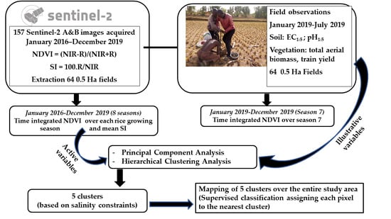
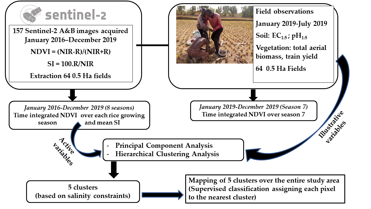
2. Materials and Methods

2.1. Study Area

The study area corresponded to the irrigated systems of Sébéri and Tchagriré (6.5 km2), located in the Niger River basin 50 km southeast of Niamey, the capital of Niger (13°16′35.32″ N, 2°21′31.81″ E) (Figure 1). The climate of the area corresponds to the dry tropical zone of the Sudano–Sahelian type. Annual precipitation has high spatial, temporal and interannual variability and a general trend towards a southward shift of isohyets over the past 30 years. Mean annual precipitation is ca. 510 mm/year (standard deviation (SD) = 100 mm/year) (National Meteorological Service of Niger). Precipitation is irregularly distributed in space and time: it peaks in August (150 mm) and is lowest in October (22 mm) and May (20 mm). Mean monthly temperature is 36 °C during the hottest period (April), with a maximum temperature of 47 °C. Minimum mean monthly temperatures are 25 °C and are observed from December to January. Evaporation varies from 1700 to 2100 mm/year. The water deficit is thus large during the dry season and is accentuated by the Harmattan, a dry continental trade wind from the Sahara. Consequently, the study area has two seasons: a dry season from October to May and a wet season from June to September [17].
Paddy fields in Sébéri and Tchagriré are located on the lowest alluvial terrace of the Niger Valley (Figure 1). The soils are Vertisols (60–74% clay in topsoil and 52–85% in subsoil) but also acidic, with a pH in water of 4.0–6.2 (SD = 0.5), an EC of 0.01–7.20 dS.m−1 (SD = 2.3 dS.m−1), and they have low hydraulic conductivity at water saturation, which ranges from 2.8 × 10⁻⁸ in the topsoil horizon to 1.5 × 10⁻⁸ m s−1 at a depth of 50 cm [18,19]. In Sébéri, EC generally increases from the areas next to the sand dunes to the river’s floodwater protection dike [19]. The types of salts found are hexahydrite, gypsum, epsomite and, secondarily, wattevilleite and sodium carbonate hydrate [19].
The observed long-term downward trend in rice yields can be explained by several factors: poor management of agricultural equipment, lack of technical supervision, soil degradation due to salinity and failure to respect the cropping calendar. Implementing a fixed and common cropping calendar for all rice-growing systems would create two growing seasons per year during optimal climatic conditions. It provides for two harvests, one in the dry cropping season (mid-November to mid-May) and the other in the wet cropping season (mid-June to mid-December) (Figure 2).

2.2. Field Data Collection Strategy

In the Niger River basin, rice is grown in 0.25 ha (25 m × 100 m) fields. We selected 44 and 20 fields in the Sébéri and Tchagriré irrigated systems, respectively, for data collection on two dates in the 2019 dry season, each of which corresponded to a date when the Sentinel-2 satellite passed over the study area. We chose the 64 fields based on the level of salinity in the study area and whether they were cultivated with rice or bare. Three sampling plots of 1 m2 each were set up on one diagonal of each of the 0.25 ha fields selected to collect soil and phenological parameters.
The first data collection campaign was performed on 8 February 2019, near the start of the growing season, when fields were already flooded and covered by a layer of irrigation water a few centimeters thick. The phenology of rice plants was assessed in a quarter (0.25 m2) of each 1 m2 plot. Then, all aerial biomass of this quarter was cut, weighed and dried under laboratory conditions to determine dry matter. The topsoil (0–30 cm) was sampled in each plot using an auger, and one composite sample per field was obtained by carefully mixing the three elementary plot samples. Given the rapidity of auger sampling and the very low hydraulic conductivity of these clay soils, sampling under a water layer did not significantly change the EC and pH values of the soil, as shown in previous studies performed in these irrigated systems [19]. Consequently, salt losses during soil sampling are very low, ensuring good reliability of collected samples and good representativeness of soil salinity measurements. The composite samples were air-dried and ground to pass through a 2-mm sieve. Then, pH in water (pH1:5) and EC in water (EC1:5) were analyzed in the laboratory following ISO 10390 and ISO 11265, respectively.
The second data collection campaign was performed on 4 May 2019, during the harvest period, when fields were not flooded. Phenological assessment and soil sampling were identical to those during the first campaign. Moreover, rice grain was collected from an undisturbed 0.25 m2 quarter to estimate grain yield. Soil and phenological parameters were analyzed statistically for each field.

2.3. Remote-Sensing Data Collection

Remote-sensing data and in situ observations were processed in multiple steps (Figure 3). First, optical images were obtained from Sentinel-2 satellites. The Sentinel-2 mission is a constellation of two satellites that are 180° out-of-phase on the same orbit, which increases the frequency of passes over a given location (i.e., every five days). Each satellite records 13 bands, with three spatial resolutions: blue, green, red and near-infrared bands at 10 m resolution; red-edge and mid-infrared bands at 20 m resolution; and aerosol and water-vapor bands at 60 m resolution. Sentinel-2′s utility thus lies in its high revisit frequency and high spatial resolution.
All existing pre-processed Sentinel-2 images from January 2016 to December 2019 were downloaded. Pre-processing was performed by the MACCS (Multi-sensor Atmospheric Correction and Cloud Screening) processing chain, which consists of three successive steps: (i) cloud detection (using the satellite cirrus band), (ii) aerosol-thickness estimation and (iii) atmospheric correction. This processing chain, developed by CESBIO and CNES, provides ortho-rectified atmospheric-corrected surface reflectance images of 100 km × 100 km as a final product [21].
Overall, 157 preprocessed Sentinel-2 images were downloaded and then resampled at a spatial resolution of 10 m. Reflectance values that were missing due to cloud cover were estimated as the mean reflectance value of the two dates before and after the missing date. Finally, the study area of the irrigated systems of Sébéri and Tchagriré was extracted from the entire image.
A second step consisted of distinguishing the periods during which a plot was bare or covered with vegetation. To do this, the NDVI was first calculated per pixel (Table 1) [22], and then the mean and standard deviation of the NDVI of each plot’s pixels was calculated. A pixel was considered to be part of a plot if its centroid fell within the plot’s polygon. Since the plots measured 25 m × 100 m, each contained ca. 25 pixels. Based on the literature [23,24], plots with a mean NDVI ≤0.21 or >0.21 were considered as bare soil or vegetation, respectively.
Means and standard deviations of NDVI were used to create a 4-year time series of NDVI for each plot. For the periods when the plots were estimated to be bare, we calculated an SI [25] (Table 1). Otherwise, for the periods when vegetation was dominant, we created a time series of NDVI over the four years of study.
A few days before rice planting and during the first part of the vegetation development cycle, a water layer covers the soil. This layer is thin, no more than a few centimeters thick, and has high turbidity. The NDVI of this water layer ranges from 0.10–0.21 before planting and then decreases as the rice is transplanted and the vegetation canopy develops. In comparison, NDVI values of the river near the plots are negative and close to −0.3.
The last step consisted of calculating the time-integrated NDVI (TI-NDVI) [26,27] for each growing season for fields with vegetation. TI-NDVI for a given growing season was calculated as follows:
T I - N D V I = t = d 1 d e 1 n i = 1 n N D V I i , t + N D V I i , t + 1 2 0.21 × d t + 1 d t
where d1 and de are the day of the year of the start and end (harvest) of the growing season (the same for all fields), respectively; d(t) is the day of the year of date t for the set of days for which Sentinel-2 images are available during the growing season; n is the number of pixels within the field; and N D V I i , t is the NDVI of pixel i on date t. Units of TI-NDVI are expressed as NDVI.days.
Figure 4 illustrates the calculation of TI-NDVI for two successive growing seasons in 2019 derived from NDVI estimates based on existing Sentinel-2 images.

2.4. Multidimensional Analysis of the Data

Principal component analysis (PCA) was performed using the FactoMiner package in R software [28] to analyze the multidimensional space of the remote-sensing and field data from 2019. Field data were pH and EC at the start and end of the growing seasons, aerial biomass and grain yields of the 64 fields. Qualitative variables were added: pH class, salinity class, land use and position in relation to the direction of river flow. Remote-sensing data were the mean SI of each field, TI-NDVI of each of the eight growing seasons and the number of seasons that each field was used to produce rice in dry and wet seasons. Remote-sensing data were considered as active variables and field data as illustrative variables.
PCA was followed by hierarchical clustering analysis (HCA) using the module HCPC (hierarchical clustering on principal components) [29] in R software [30] to create clusters of fields that behaved similarly. Finally, supervised classification for grids (SCG) was applied to 10-m resolution grids of the entire area that described the remote-sensing variables used in the PCA-HCA analysis (i.e., 8 grids with the TI-NDVI of each pixel for the 8 seasons and 1 grid with the SI of each pixel) to represent the spatial distribution of the clusters. Each pixel is assigned to the cluster with the shortest Mahalanobis distance, and the distance to the nearest cluster is analyzed to assess the quality of assignment to a cluster. SAGA-GIS 2.3.2 [31], implemented in QGIS 3.4.3, was used to perform the SCG with a maximum-likelihood algorithm.

3. Results

3.1. NDVI Dynamics over the Eight Growing Seasons

Figure 5 shows the dynamics of mean NDVI estimated from the 25 pixels within each of the three fields. The threshold of NDVI = 0.21 was selected to identify periods without live vegetation, and it enabled the identification of the short intercropping period after harvest when field irrigation was stopped, the soil plowed and irrigation started again before transplanting the next rice crop.
Non-cultivated fields had NDVI dynamics below the threshold or slightly above due to weed growth (Figure 5a). When cultivated during a growing season, some fields had lower NDVI due to constrained plant growth, which could have been due in part to soil salinity. Among the fields cultivated during both dry and wet seasons, two groups of cultivated fields were identified: (i) those with lower NDVI during the dry seasons than wet seasons (Figure 5b) and (ii) those with smaller differences between dry and wet seasons and generally high NDVI (Figure 5c).

3.2. Spatial Variation in TI-NDVI over the Eight Growing Seasons

For the 8 seasons and 44 irrigated fields monitored in Sébéri, TI-NDVI was always significantly lower during dry seasons than wet seasons (Figure 6a): mean TI-NDVI per season ranged from 15 to 19 NDVI.days during the four dry seasons and 29 to 34 NDVI.days during the four wet seasons. TI-NDVI also varied greatly among fields for a given season and showed systematic trends, with values frequently lower in some fields in the south and northwest of the irrigation system and significantly higher in fields in the center (Figure 6b). This spatial variation was lower in some seasons (e.g., seasons 2 and 6) but higher in others, e.g., season 7 in 2019, when field data were collected.

3.3. Salinity Measured in the Field in 2019

For the 64 fields monitored in 2019 during the dry season, EC1:5 ranged from 0.01 to 5.36 dS/m at the start of the season and 0.44 to 6.19 dS/m at the end of the season (SD = 1.16 and 1.33 dS/m, respectively) (Table 2). The pH ranged from 5.52 to 6.68 in January and 5.29–6.25 in June (SD = 0.44 and 0.52, respectively). Differences between means and SDs for the two dates were not significant for EC1:5 or pH. Total aerial biomass and grain yield at harvest varied greatly (Table 2), and 18 fields had no rice production.

3.4. Correlation between Remote-Sensing Data and Field Data during the 2019 Dry Season

A strong and significant (p < 0.05) positive correlation was observed between TI-NDVI in season 7 and both total aerial biomass (r = 0.77, p < 2 × 10¹⁴) and grain yield (r = 0.82, p < 2.2 × 10¹⁶) (Table 3), which confirms that TI-NDVI is a good indicator of rice vegetation growth and its final yield. Soil EC1:5 was negatively correlated with TI-NDVI at the start and end of the season (r = −0.38, p = 0.002 for the start, p = 0.002 for the end), with total biomass (r = −0.23, p = 0.062) and, significantly, with grain yield (r = −0.29, p = 0.019).

3.5. PCA and HCA Analysis of Remote-Sensing Data over the Eight Growing Seasons

The first axis of the PCA was positively correlated with all of the TI-NDVI variables (Figure 7), which indicates that the spatial variability in TI-NDVI among fields was the main factor that influenced variations in the dimensional space. The second axis was correlated with SI but also distinguished the TI-NDVI estimates of the dry seasons (1, 3, 5 and 7) from those of the wet seasons (2, 4, 6 and 8).
While soil pH was little represented in the first PCA plane, soil EC1:5 measured at the start and end of season 7 was negatively correlated with the first axis and thus with TI-NDVI variables. More surprisingly, neither soil EC1:5 variable was correlated with SI. Following PCA, HCA identified five clusters of fields that behaved similarly during the eight growing seasons according to the remote-sensing data (Figure 8).

3.6. Description of the Field Clusters

The five clusters differed in their remote-sensing and field data (Table 4):
  • Cluster 1 had low TI-NDVI in both dry and wet seasons. In 2019, EC1:5 was highest in this cluster, soil pH was very acidic and total biomass and grain yield were zero. The maximum EC1:5 of some fields in this cluster (5.36 dS/m) indicates that this cluster had the highest salinity.
  • Cluster 2 had low TI-NDVI in dry seasons, due to rare cultivation, and a higher TI-NDVI in wet seasons, but one that was still lower than those of clusters 3–5. In 2019, soil EC1:5 was not significantly higher than those of clusters 3–5, but total biomass and grain yield were significantly lower.
  • Cluster 3 had moderate TI-NDVI in dry and wet seasons and a significantly higher SI. In 2019, soil EC1:5 was low, pH was relatively high, and mean total biomass and grain yield were the second highest among the clusters.
  • Cluster 4 had low TI-NDVI in dry seasons due to frequent non-cultivation but high TI-NDVI in wet seasons. In 2019, soil EC1:5 and pH were low, and the fields were not cultivated.
  • Cluster 5 had extremely high TI-NDVI in both dry and wet seasons. In 2019, soil EC1:5 was low, pH was relatively high and total biomass and grain yield were the highest.

3.7. Mapping the Clusters over the Entire Study Area

Using the eight grids with the TI-NDVI of each pixel for the eight seasons and the grid with the SI of each pixel, SCG enabled each pixel to be attached to one of the five clusters defined from the 64 study fields considered as training areas. Figure 9 shows the distribution of the five clusters over the entire study area, with the associated distance to the nearest cluster, which indicates when the cluster represents a given pixel well (i.e., small distance) or poorly (i.e., large distance). Clusters 1 and 2, both of which had low TI-NDVI during the dry seasons since they were often not cultivated, were located mainly in the north and south of the Sébéri system (Figure 9). Cluster 5, with the highest TI-NDVI in both dry and wet seasons, predominated in the north of the Tchagriré system and the center of the Sébéri system. Cluster 3, with moderate TI-NDVI in both seasons, represented large areas in Sébéri in intermediate positions between clusters 1 or 2 and 5, but also in non-agricultural areas (e.g., paths, natural areas), which had large distances to the nearest cluster. Cluster 4 occupied small areas in Sébéri and the south of Tchagriré, often near fields of cluster 2.

4. Discussion

This study continuously monitored spatio-temporal dynamics of SI and NDVI in paddy fields using Sentinel-2 satellite images over eight growing seasons from 2016 to 2019. Based on field data collected (biomass, EC and pH) during the 2019 dry growing season, a relation between spectral indices (NDVI and SI) and field data was established to understand the behavior of rice crops and relate the spatio-temporal variation and pattern of spectral indices to salinity.

4.1. Variation in Spectral Indices among Crop Seasons

In the 2016–2019 time series, the spectral indices used (SI and NDVI) varied in different ways. First, SI was estimated at dates when bare soils prevailed according to an NDVI threshold (NDVI <0.21). SI averaged over the 4 years of study varied in a narrow range and was weakly correlated with soil EC1:5; only highly saline areas, generally not cultivated, had higher SI values, due to the presence of salt crusts at the surface. These results may be explained by the short periods during which bare soil can be observed in irrigated paddy field systems; they generally last less than a month between successive crops, which corresponded to 3–5 dates when Sentinel-2 images were available. Thus, only a few dates when SI could be estimated were available. The soil may also be covered by crop residues or change drastically in water content due to the stopping or starting of irrigation after harvest or before preparatory work for planting rice. These factors may interfere with the estimation of SI and limit its ability to distinguish soil salinity.
In contrast, NDVI dynamics could be followed at a fine temporal resolution since cloud-free images were available at 133 dates during the eight growing seasons, with a mean of 21 dates per season since the end of 2017. We observed significant differences in TI-NDVI among the fields and eight growing seasons. TI-NDVI, which differed greatly between fields in a given season and over time, was used to differentiate areas with constraints to vegetation growth in the irrigated systems. In a given season, non-cultivated or cultivated areas with constraints had low TI-NDVI in dry and wet seasons (clusters 1 and 2) (Table 4). Areas cultivated throughout the year with few constraints had high TI-NDVI in wet seasons and moderate TI-NDVI in dry seasons (cluster 3), while zones cultivated in dry and wet seasons without any constraints had high TI-NDVI in both seasons (cluster 5) (Figure 8). Nonetheless, there were areas near the main drainage channel with salinity constraints and moderate TI-NDVI that were cultivated only in wet growing seasons. They may have occurred because they are always wet and wild grasses grow there in the dry seasons, which influences the NDVI. TI-NDVI also differed significantly between dry and wet seasons (Figure 5a,b). Wet growing seasons had higher mean TI-NDVI than dry ones. TI-NDVI varied from 29 to 34 NDVI.days in wet seasons and 15 to 19 NDVI.days in dry seasons. This result is due to the climatic conditions in the study area in dry seasons (hot, dry wind, high temperature) that limit crop growth. In addition, high temperature favors the rise of salt from lower horizons to the rooting zone of crops, which damages their roots. In wet seasons, conditions are more favorable for crop growth. Over the time series, wet and dry seasons varied among years, again due to climatic conditions (temperature in dry seasons and precipitation in wet seasons).

4.2. Temporal and Spatial Patterns of NDVI

Soil salinity influences vegetation density and crop growth, as explained by NDVI. TI-NDVI was used in this study to indicate constraints to crop growth and density, as in previous studies [32]. Five clusters were obtained to differentiate areas with constraints to rice growth in the two irrigated systems. Non-cultivated areas had the lowest TI-NDVI and were considered likely to be areas with high salinity constraints (cluster 1) (Figure 9). Areas cultivated only in wet seasons because of constraints had low TI-NDVI and may be considered to have moderate salinity constraints that limit crop growth (clusters 2 and 4) (Figure 9). Areas cultivated in both seasons with few constraints had high TI-NDVI and may be considered to have few salinity constraints (cluster 3) (Figure 9). Finally, areas cultivated without constraints had the highest TI-NDVI (cluster 5) (Figure 9) and were considered zones without salinity constraints. Our results show that the spatial pattern of TI-NDVI corresponds to the spatial distribution of problematic patches in the study area. The main constraint may be salinity, while other constraints could be explained by soil type, microtopography and farming practices. Mean ECe measured during ground truthing was calculated for each cluster and assigned to the respective TI-NDVI of the clusters to validate the four salinity classes obtained from the classification of TI-NDVI. Based on EC measurements, visual observations and knowledge of the terrain [33], mean TI-NDVI of the clusters were classified into four classes of soil salinity [34]: non-saline, slightly, moderately and very saline (i.e., ECe < 2, 2–4, 4–8 and 8–16 dS/m, respectively). Measured soil EC alone could not explain the level of salinity of the clusters (Table 4); however, integrated interpretation using the EC, mean TI-NDVI, total biomass and grain yield with visual observations of the study area could be used. Cluster 1, consisting of abandoned fields with low mean TI-NDVI in dry and wet seasons, no rice biomass or grain yield, maximum EC of 5.36 dS/m2 and white efflorescence on the soil surface, can be considered saline soil. Clusters 2 and 4, consisting of fields cultivated only in wet seasons and rarely in dry seasons, despite having a lower level of surface salinity, have low TI-NDVI in dry seasons, low biomass and grain yield in the few fields cultivated in dry seasons and no yield in non-cultivated fields. Salt efflorescence is present in these fields. The maximum EC was 2.59 dS/m2, which may not reflect the true EC of the clusters. These two clusters can be considered moderately saline. Clusters 3 and 5 consisted of cultivated fields in both dry and wet seasons. Based on measured EC, they were classified as non-saline, but since cluster 3 has lower TI-NDVI, biomass and grain yields than cluster 5, cluster 3 has few salinity constraints. Thus, cluster 3 can be considered slightly saline and cluster 5 non-saline.

4.3. Field EC Variation and Salinity

In the Sébéri irrigated system, EC generally increased from the areas next to the sand dunes to the river’s floodwater protection dike, perhaps because the dike has modified the functioning of the soils next to it [18]. In the Tchagriré irrigated system, EC generally increased from the areas next to the river to the main drainage ditch, likely due to topography. Areas at lower elevations had higher EC than those at higher elevations. Overall, the pattern of EC followed those of TI-NDVI, biomass and grain yield. EC measured in the two systems does not reflect the real situation in the field. Areas that showed signs of salinity (i.e., abandoned fields, low NDVI, low yields) had low measured EC, which indicates that a salt stock may lie in the lower horizons. To map salinity in this situation, measured EC should be compared to other maps (e.g., TI-NDVI, yield, soil, elevation) of the same site with similar sampling patterns or resolution. Doing so may provide useful insights into other parameters that could explain salinity.

5. Conclusions

This study developed a step-by-step method to estimate constraints on the growth of rice, the most important of which is salinity. Dense time series of Sentinel-2 images over eight growing seasons enabled us to describe the behavior of rice biomass and to differentiate fields where rice is subjected to stress during growing seasons. In irrigated systems, periods of bare soil were brief, and the SI derived from Sentinel-2 images could not differentiate soil salinity of fields. Monitoring vegetation behavior over four years by deriving the NDVI from Sentinel-2 images and calculating the TI-NDVI was able to differentiate fields based on constraints that limit rice growth. Several constraints can occur in areas subjected to stresses but can be related locally to soil salinity and verified by field sampling, which can be guided by TI-NDVI classification. This approach is particularly adapted to irrigated rice systems in which monoculture prevails and differences in TI-NDVI are not caused by different crops.

Author Contributions

I.M., C.W. and D.M. conceived the topic and developed the method. P.P. performed the technical work of downloading and processing images and calculating spectral indices. I.M., C.W. and D.M. wrote the manuscript, which was improved by H.N., Y.G. and I.A.B. participated actively in the fieldwork. All authors have read and agreed to the published version of the manuscript.

Funding

This study was made possible thanks to financial support of the EU-funded Agrocampus ERASMUS+ cooperation project in Rennes, France. This program financed a one-year’s internship for M.I. and his supervision.

Acknowledgments

This study was performed with the administrative and technical support of the soil science laboratory from UMR SAS, INRAE and Institut Agro.

Conflicts of Interest

The authors declare no conflict of interest.

References

  1. World Water Assessment Programme (WWAP). Fact 24: Irrigated Land. United Nations Educational, Scientific and Cultural Organization (UNESCO). Available online: http://www.unesco.org/new/en/natural-sciences/environment/water/wwap/facts-and-figures/all-facts-wwdr3/fact-24-irrigated-land/ (accessed on 26 August 2020).
  2. Barbiéro, L.; Van Vliet-Lanoe, B. The alkali soils of the middle Niger valley: Origins, formation and present evolution. Geoderma 1998, 84, 323–343. [Google Scholar] [CrossRef] [Green Version]
  3. Guéro, Y. Organisation et Propriétés Fonctionnelles des sols de la Vallée du Moyen Niger. Ph.D. Thesis, Tunis University, Tunis, Tunisia, Niamey University, Niamey, Niger, 1987. [Google Scholar]
  4. Munns, R.; Cramer, G.R.; Ball, M.C. Interactions between Rising CO2 Soil Salinity, and Plant Growth. In Carbon Dioxide and Environmental Stress; Luo, Y., Mooney, H.A., Eds.; Academic Press: Cambridge, MA, USA, 1999; pp. 139–167. [Google Scholar]
  5. Shrivastava, P.; Kumar, R. Soil salinity: A serious environmental issue and plant growth promoting bacteria as one of the tools for its alleviation. Saudi J. Biol. Sci. 2015, 22, 123–131. [Google Scholar] [CrossRef] [PubMed] [Green Version]
  6. Pessarakli, M.; Szabolcs, I. Soil Salinity and Sodicity as Particular Plant/Crop Stress Factors. In Handbook of Plant and Crop Stress, 2nd ed.; Pessarakli, M., Ed.; Marcel Dekker, Inc.: New York, NY, USA, 1999; ISBN 978-0-8247-1948-7. [Google Scholar]
  7. Maas, E.V.; Grattan, S.R. Crop Yields as Affected by Salinity. In Agronomy Monographs; Skaggs, R.W., van Schilfgaarde, J., Eds.; American Society of Agronomy: Madison, WI, USA, 2015; pp. 55–108. ISBN 978-0-89118-230-6. [Google Scholar]
  8. Mougenot, B.; Pouget, M.; Epema, G.F. Remote sensing of salt affected soils. Remote Sens. Rev. 1993, 7, 241–259. [Google Scholar] [CrossRef]
  9. Scudiero, E.; Skaggs, T.H.; Corwin, D.L. Regional scale soil salinity evaluation using Landsat 7, western San Joaquin Valley, California, USA. Geoderma Reg. 2014, 2–3, 82–90. [Google Scholar] [CrossRef]
  10. Scudiero, E.; Skaggs, T.H.; Corwin, D.L. Comparative regional-scale soil salinity assessment with near-ground apparent electrical conductivity and remote sensing canopy reflectance. Ecol. Indic. 2016, 70, 276–284. [Google Scholar] [CrossRef] [Green Version]
  11. Metternicht, G.I.; Zinck, J.A. Remote sensing of soil salinity: Potentials and constraints. Remote Sens. Environ. 2003, 85, 1–20. [Google Scholar] [CrossRef]
  12. Nicolas, H.; Walter, C. Detecting salinity hazards within a semiarid contextby means of combining soil and remote-sensing data. Geoderma 2006, 134, 217–230. [Google Scholar]
  13. Wang, J.; Ding, J.; Yu, D.; Ma, X.; Zhang, Z.; Ge, X.; Teng, D.; Li, X.; Liang, J.; Lizaga, I.; et al. Capability of Sentinel-2 MSI data for monitoring and mapping of soil salinity in dry and wet seasons in the Ebinur Lake region, Xinjiang, China. Geoderma 2019, 353, 172–187. [Google Scholar] [CrossRef]
  14. Tripathi, N.K.; Rai, B.K.; Dwivedi, P. Spatial modeling of soil alkalinity in GIS environment using IRS data. In Proceedings of the 18th Asian Conference on Remote Sensing, Kuala Lumpur, Malaysia, 20–24 October 1997. [Google Scholar]
  15. Khan, N.M.; Rastoskuev, V.V.; Sato, Y.; Shiozawa, S. Assessment of hydrosaline land degradation by using a simple approach of remote sensing indicators. Agric. Water Manag. 2005, 77, 96–109. [Google Scholar] [CrossRef]
  16. Gorji, T.; Sertel, E.; Tanik, A. Monitoring soil salinity via remote sensing technology under data scarce conditions: A case study from Turkey. Ecol. Indic. 2017, 74, 384–391. [Google Scholar] [CrossRef]
  17. Food and Agriculture Organization. AQUASTAT Profil de Pays-Niger; Organisation des Nations Unies pour l’Alimentation et l’Agriculture: Rome, Italie, 2015; p. 18. [Google Scholar]
  18. Guéro, Y. Contribution à L’étude des Mécanismes de Dégration Physico-Chimique des sols Sous Climat Sahélien: Exemple pris Dans la Vallée du Moyen Niger. Ph.D. Thesis, Université de Niamey, Niamey, Niger, 2000. [Google Scholar]
  19. Adam, I. Cartographie Fine et Suivi Détaillé de la Salinité des sols d’un Périmètre Irrigué au Niger en vue de leur Remédiation. Ph.D. Thesis, Uiversité de Bretagne Occidentale, Brest, France, Université Abdou Moumouni de Niamey, Niamey, Niger, 2011. [Google Scholar]
  20. Ndanga Kouali, G.; Lévite, H.; Anid, M. Diagnostic Participatif Rapide et Planification des Actions du Périmètre de Daïbéri (Département de Tillabéri-NIger); Technical Report; l’Association Nigérienne pour l’Irrigation et le Drainage (ANID): Niamey, Niger, 2010; p. 58. [Google Scholar]
  21. Hagolle, O.; Huc, M.; Desjardins, C.; Auer, S.; Richter, R. MAJA Algorithm Theoretical Basis Document; Technical Report; CNES, CESBIO and DLR: Berlin, Germany, 2017. [Google Scholar]
  22. Rouse, J.W.; Haas, R.H.; Schell, J.A.; Deering, D.W.; Harlan, J.C. Monitoring the Vernal Advancement of Retrogradation of Natural Vegetation, Type III, Final Report; NASA/GSFC: Greenbelt, MD, USA, 1974; pp. 1–137. [Google Scholar]
  23. Shabou, M.; Mougenot, B.; Chabaane, Z.; Walter, C.; Boulet, G.; Aissa, N.; Zribi, M. Soil Clay Content Mapping Using a Time Series of Landsat TM Data in Semi-Arid Lands. Remote Sens. 2015, 7, 6059–6078. [Google Scholar] [CrossRef] [Green Version]
  24. Roussillon, J. Développement de Méthodes Innovantes de Cartographie de L’occupation du sol à Partir de Séries Temporelles D’images Haute Résolution Visible (NDVI). Master’s Thesis, Le Mans Université, Le Mans, France, 2015. [Google Scholar]
  25. Allbed, A.; Kumar, L.; Aldakheel, Y.Y. Assessing soil salinity using soil salinity and vegetation indices derived from IKONOS high-spatial resolution imageries: Applications in a date palm dominated region. Geoderma 2014, 230–231, 1–8. [Google Scholar] [CrossRef]
  26. Ma, C.; Guo, Z.; Zhang, X.; Han, R. Annual integral changes of time serial NDVI in mining subsidence area. Trans. Nonferrous Met. Soc. China 2011, 21, s583–s588. [Google Scholar] [CrossRef]
  27. Reed, B.C.; Brown, J.F.; VanderZee, D.; Loveland, T.R.; Merchant, J.W.; Ohlen, D.O. Measuring phenological variability from satellite imagery. J. Veg. Sci. 1994, 5, 703–714. [Google Scholar] [CrossRef]
  28. Husson, F.; Josse, J.; Pages, J. Principal Component Methods—Hierarchical Clustering—Partitional Clustering: Why Would We Need to Choose for Visualizing Data? Technical Report; Agrocampus: Angers, France, 2010. [Google Scholar]
  29. Husson, F.; Josse, J.; Pagès, J. Analyse de données avec R-Complémentarité des méthodes d’analyse factorielle et de classification. In Proceedings of the 42èmes Journées de Statistique, Marseille, France, 25–29 May 2010. [Google Scholar]
  30. R Core Team. European Environment Agency. Available online: https://www.eea.europa.eu/data-and-maps/indicators/oxygen-consuming-substances-in-rivers/r-development-core-team-2006 (accessed on 26 August 2020).
  31. Conrad, O.; Bechtel, B.; Bock, M.; Dietrich, H.; Fischer, E.; Gerlitz, L.; Wehberg, J.; Wichmann, V.; Böhner, J. System for Automated Geoscientific Analyses (SAGA) v. 2.1.4. Geosci. Model Dev. 2015, 8, 1991–2007. [Google Scholar] [CrossRef] [Green Version]
  32. Kundu, A.; Denis, D.; Patel, N.; Dutta, D. A Geo-spatial study for analysing temporal responses of NDVI to rainfall. Singap. J. Trop. Geogr. 2018, 39, 107–116. [Google Scholar] [CrossRef]
  33. Abbas, A.; Khan, S.; Hussain, N.; Hanjra, M.A.; Akbar, S. Characterizing soil salinity in irrigated agriculture using a remote sensing approach. Phys. Chem. Earth Parts A/B/C 2013, 55–57, 43–52. [Google Scholar] [CrossRef]
  34. Shahid, S.; Rahman, K. Soil Salinity Development, Classification, Assessment, and Management in Irrigated Agriculture. In Handbook of Plant and Crop Stress, 3rd Ed.; Pessarakli, M., Ed.; CRC Press: Boca Raton, FL, USA, 2011; Volume 20102370, pp. 23–39. ISBN 978-1-4398-1396-6. [Google Scholar]
Figure 1. Location of the study area and aerial view of the experimental fields in the Sébéri and Tchagriré irrigation systems south of Niamey (Niger).
Remotesensing 12 03399 g001
Figure 2. Double-cropping calendar for rice in the middle Niger valley (adapted from [20]).
Remotesensing 12 03399 g002
Figure 3. General data-processing flowchart.
Remotesensing 12 03399 g003
Figure 4. Example of normalized difference vegetation index (NDVI) dynamics for a given field for the dry and wet seasons of 2019 (derived from 42 cloud-free images among 60 existing Sentinel-2 images) and time-integrated NDVI (TI-NDVI) calculation for the two growing seasons.
Remotesensing 12 03399 g004
Figure 5. Example of dynamics of mean NDVI for three fields over eight growing seasons from January 2016 to December 2019: (a) Field CP3_1, cultivated in season 2 but not in the other seasons; (b) Field CP11-1, always cultivated but with lower NDVI in dry seasons than wet seasons; and (c) Field TVP7, always cultivated and with high NDVI in both dry and wet seasons. For each field, mean NDVI and its 95% confidence interval were estimated from the field’s ca. 25 pixels.
Remotesensing 12 03399 g005
Figure 6. Temporal and spatial variations in the time-integrated normalized difference vegetation index (TI-NDVI) for the 44 fields of the Sébéri irrigation system: (a) mean and standard deviation of TI-NDVI for each season; (b) maps of TI-NDVI estimated for the eight growing seasons.
Remotesensing 12 03399 g006
Figure 7. First plane of principal component analysis with variables derived from remote sensing as active variables (black) and soil and vegetation variables as illustrative variables (blue). Abbreviations: TI-NDVI_SN: time-integrated normalized difference vegetation index for season N; Mean_SI: mean salinity index; biom_yield: biomass yield at harvest; grain yield: grain yield at harvest; Soil EC_start_s: soil electrical conductivity at the start of the season; soil EC_end_s: soil electrical conductivity at the end of the season; soil pH_start_s: soil pH at the start of the season; Soil pH_end_season: soil pH at the end of the season; Nbr_dry_s: number of dry growing seasons during the time series; and Nbr_wt_s: number of wet growing seasons during the time series.
Remotesensing 12 03399 g007
Figure 8. Representation on the first plane of principal component analysis (PCA) of the five clusters of fields defined by ascending hierarchical classification applied to the first three axes of the PCA. Points are labeled with field codes starting with S or T respectively for Seberi or Tchagrire irrigation system, while squares indicate barycenters of clusters.
Remotesensing 12 03399 g008
Figure 9. Mapping of the five clusters over the entire study area of the irrigated systems of Sébéri and Tchagriré using supervised classification that assigned each pixel to the nearest cluster.
Remotesensing 12 03399 g009
Table 1. Characteristics and equations of the bare soil and vegetation indices selected. RED and NIR indicate red and near-infrared bands of the Sentinel-2 images.
Spectral IndexEquationCharacteristics
Salinity index (SI)SI = (RED/NIR) × 100 in [25] Created to detect saline soils.
Normalized difference vegetation index (NDVI)NDVI = (NIR − RED)/(NIR + RED) [22]
Varies from −1.0 to +1.0.For vegetation, NDVI varies from 0.2–0.8.
A standardized index for vegetation cover and chlorophyll activity. Used to monitor drought and monitor and predict agricultural production.
Table 2. Statistics of field data for the dry growing season in 2019 (i.e., season 7) (n = 64, including 18 non-cultivated fields).
Soil EC1:5 (dS/m)Soil pH1:5Total Aerial Biomass (g/m²)Grain Yield (g/m²)
StatisticStart of
Season
At
Harvest
Start of
Season
At HarvestAt
Harvest
At
Harvest
Mean0.400.445.525.29914.2389.5
Median0.030.045.565.331048.5420
SD1.161.330.440.52687.8309.0
Min0.010.014.454.0000
Max5.366.196.686.2522691249
Table 3. Pearson correlations between the TI-NDVI indicator derived from Sentinel-2-images and soil (EC1:5, pH1:5) and crop indicators (total biomass, grain yield). Data were collected for 64 fields during the dry season of 2019 (i.e., season 7). SS and ES indicate the start and end of the growing season, respectively. Bold values indicate significant (p < 0.05) correlations.
TI-NDVISoil EC1:5 SS Soil EC1:5
ES
Soil pH
SS
Soil pH
ES
Total Aerial Biomass Grain
Yield
TI-NDVI1.00
Soil EC1:5_SS −0.381.00
Soil EC1:5_ES −0.380.991.00
Soil pH SS 0.35−0.63−0.631.00
Soil pH_ES 0.16−0.62−0.620.741.00
Total Aerial
Biomass
0.77−0.23−0.230.350.11.00
Grain Yield0.82−0.29−0.280.340.070.721.00
Table 4. Mean (and standard deviation) per cluster of fields defined by ascending hierarchical clustering for the variables derived from Sentinel-2 images (TI-NDVI, SI) and from field data collected in 2019 (EC1:5, pH, total biomass, grain yield). For each variable, different letters indicate significant differences in the mean among clusters according to a p < 0.05 Tukey test at a 95% confidence level.
2016–2019Dry Season 2019
ClusterNo. of FieldsDry Season TI-NDVI
(NDVI.Days)
Wet Season TI-NDVI
(NDVI.Days)
Mean SISoil EC1:5
(dS/m)
Soil pHTotal Biomass
(g/m2)
Grain Yield
(g/m2)
171.0 (1.2) a12.8 (4.4) a72.9 (3.0) ab2.6 (2.4) b5.0 (0.6) a0 (0) a0 (0) a
295.2 (6.1) b25.5 (3.1) b72.5 (2.4) a0.6 (1.1) a5.5 (0.2) bc314 (572) a109 (217) a
31419.7 (3.6) d30.6 (1.8) c74.8 (1.3) b0.1 (0.0) a5.7 (0.2) c1308 (319) b527 (179) b
4610.1 (4.0) c44.6 (5.0) e70.1 (0.9) a0.1 (0.0) a5.2 (0.3) ab0 (0) a0 (0) a
52825.4 (1.9) e35.9 (3.1) d75.0 (1.7) b0.05 (0.1) a5.6 (0.4) bc1335 (414) b592 (205) b
Publisher’s Note: MDPI stays neutral with regard to jurisdictional claims in published maps and institutional affiliations.

