Article

Quantitative Soil Wind Erosion Potential Mapping for Central Asia Using the Google Earth Engine Platform

1
State Key Laboratory of Desert and Oasis Ecology, Xinjiang Institute of Ecology and Geography, Chinese Academy of Sciences, Urumqi 830011, China
2
Research Center for Ecology and Environment of Central Asia, Chinese Academy of Sciences, Urumqi 830011, China
3
University of Chinese Academy of Sciences, Beijing 100049, China
4
College of Resources and Environment Sciences, Xinjiang University, Urumqi 830046, China
*
Author to whom correspondence should be addressed.
Remote Sens. 2020, 12(20), 3430; https://doi.org/10.3390/rs12203430
Submission received: 1 September 2020 / Revised: 16 October 2020 / Accepted: 16 October 2020 / Published: 19 October 2020
(This article belongs to the Special Issue Land Degradation Assessment with Earth Observation)

Abstract

:
A lack of long-term soil wind erosion data impedes sustainable land management in developing regions, especially in Central Asia (CA). Compared with large-scale field measurements, wind erosion modeling based on geospatial data is an efficient and effective method for quantitative soil wind erosion mapping. However, conventional local-based wind erosion modeling is time-consuming and labor-intensive, especially when processing large amounts of geospatial data. To address this issue, we developed a Google Earth Engine-based Revised Wind Erosion Equation (RWEQ) model, named GEE-RWEQ, to delineate the Soil Wind Erosion Potential (SWEP). Based on the GEE-RWEQ model, terabytes of Remote Sensing (RS) data, climate assimilation data, and some other geospatial data were applied to produce monthly SWEP with a high spatial resolution (500 m) across CA between 2000 and 2019. The results show that the mean SWEP is in good agreement with the ground observation-based dust storm index (DSI), satellite-based Aerosol Optical Depth (AOD), and Absorbing Aerosol Index (AAI), confirming that GEE-RWEQ is a robust wind erosion prediction model. Wind speed factors primarily determined the wind erosion in CA (r = 0.7, p < 0.001), and the SWEP has significantly increased since 2011 because of the reversal of global terrestrial stilling in recent years. The Aral Sea Dry Lakebed (ASDLB), formed by shrinkage of the Aral Sea, is the most severe wind erosion area in CA (47.29 kg/m2/y). Temporally, the wind erosion dominated by wind speed has the largest spatial extent of wind erosion in Spring (MAM). Meanwhile, affected by the spatial difference of the snowmelt period in CA, the wind erosion hazard center moved from the southwest (Karakum Desert) to the middle of CA (Kyzylkum Desert and Muyunkum Desert) during spring. According to the impacts of land cover change on the spatial dynamic of wind erosion, the SWEP of bareland was the highest, while that of forestland was the lowest.

Graphical Abstract

1. Introduction

During the past few decades, global climate change and human disturbance have meant that land degradation has become one of the most serious environmental problems of the 21st century [1]. Despite the lack of strong political will, the land degradation problem has attracted much attention throughout the world [2]. As of today, over 120 countries have committed to the Land Degradation Neutrality (LDN) Target Setting Programme, which strives to achieve a land degradation neutral world before 2030 [2]. Soil erosion is the major global soil degradation threat to land, freshwater, and oceans [3]. More than 83% of the global extent of land degradation is caused by soil erosion [4]. Because of human activities and climatic variations, the soil erosion can cause topsoil loss, which leads to land degradation requiring centuries to recover, such as soil productivity loss and the thinning out of vegetative cover [5,6].
In the arid land, wind plays a more important role than water in removing the fertile topsoil, which requires centuries to build up [1]. The escalating loss of topsoil by wind erosion is a potential threat to sustainable agriculture, which is closely related to food security [7]. The soil organic matter and several other soil nutrients in the topsoil easily blow away due to strong near-surface wind, and in turn, the soil fertility and plant productivity are decreased. According to a report from the European Soil Data Center (ESDAC), about 28% of the global land degradation area suffers from the wind-driven soil erosion process [8]. Therefore, wind erosion is considered a significant threat to food security and human health, especially in arid and semi-arid regions of the world [9,10]. In addition, the hazard of sand and dust storms is one of the most severe consequences of wind erosion. Wind-blown soil particles and chemicals that lead to air pollution can affect the human respiratory system [11]. Therefore, the ability to accurately simulate and predict soil wind erosion is essential for land degradation control, suitable agricultural management, and sandstorm prevention, especially in arid regions.
As one of the largest land-locked arid regions, Central Asia (CA) has a critical need to combat desertification [12]. Moreover, CA has suffered from the most frequent sandstorms due to the frequent strong wind, limited rainfall, low vegetation coverage, and intense human disturbance [13]. Among those factors, it is generally accepted that the near-surface wind speed plays a vital role in wind erosion dynamics [14]. The need to investigate the soil wind erosion potential over CA is of great importance and brings unique challenges of large-scale wind erosion modeling and insufficient ground measurements [15,16]. Researches on the near-surface wind speed have revealed that there has been a global declining trend of the near-surface wind speed since the 1970s, which is known as global terrestrial stilling [14,17,18,19]. Affected by global terrestrial stilling, Li, et al. [20] found that the soil wind erosion modulus exhibited a declining trend across CA between 1986 and 2005. However, recent studies found a reversal in global terrestrial stilling around 2010 [21,22,23]. Furthermore, little is known about the wind speed variability across CA after 2010, let alone the impact of the reversed stilling on the wind erosion dynamic [20,24]. Additionally, existing researches cannot produce continuous high spatial-temporal resolution near-real-time (NRT) wind erosion products of the entire CA, especially for recent years [20,25]. These kinds of wind erosion maps are critical for ecological protection and land use practice in CA.
Wind erosion is a complex physical process controlled by both natural factors and human activities, and normally includes the wind speed, soil characteristics, surface roughness, vegetation cover, agricultural activities, and so on [14,26,27,28,29,30]. It is well-established that three conditions including strong enough wind, susceptible soil surface, and no surface protection by vegetation cover or snow cover, are required for soil wind erosion to occur [31]. The measurement of wind erosion has always been a major obstacle in wind erosion research. According to the literature, two categories of prominent methods, including the 137Cs tracing technique and wind tunnel experiment, can estimate wind erosion more precisely [32,33]. However, they have limitations in that the measurement involves labor-intensive work and hardly describes the spatial variation of wind erosion. Additionally, due to the complex physical processes and driving mechanisms of wind erosion, it is still difficult to monitor the process and conduct quantitative measurements on wind erosion on a large-scale. Over the past few decades, substantial efforts have been made in terms of investigating the mechanism and driving factors of wind erosion. Based on small-scale regional field studies and wind tunnel experiments, several quantitative assessment models of wind erosion have been developed [34,35,36,37,38]. Since the scientific investigations of Bagnold [38] on the wind erosion prediction technology in 1941, soil wind erosion models ranging from empirical-based to physics-based models, have been put forward. The most accepted models developed to quantify soil wind erosion include Wind Erosion Equation (WEQ) [39], Revised Wind Erosion Equation (RWEQ) [37], Wind Erosion Prediction System (WEPS) [40], Single-event Wind Erosion Evaluation Program (SWEEP) [41], Erosion Productivity Impact Calculator (EPIC) [42], Agricultural Policy/Environmental eXtender (APEX) [43], Texas Erosion Analysis Model (TEAM) [44], and Wind Erosion on European Light Soils (WEELS) [45]. Due to the limited parameters and data that can be obtained, it is difficult for this kind of wind erosion model to simulate soil loss by wind erosion at a larger geographic scale. In contrast with others, the RWEQ model proposed by Fryrear, et al. [37] employs a set of mathematical equations to input weather, soils, crops, and tillage data. Additionally, the RWEQ model has been validated with filed erosion data from 45 site years in several US states [37]. Due to the limitations of RWEQ input data acquisition, the original RWEQ was designed to calculate wind erosion loss at a field scale [36]. Zobeck, et al. [46] evaluated the feasibility of scaling up from fields to regions to estimate the soil wind erosion potential by a geographic information system (GIS)-based field scale wind erosion model in Texas, US. Chi, et al. [47] used the RWEQ model to calculate the soil wind erosion modulus based on field sampling point data regression and remote sensing data over China. Borrelli, et al. [48] developed the GIS-RWEQ model to evaluate the soil loss potential due to wind erosion in the European Union (EU). Although the RWEQ model has achieved some success in large-scale applications, a large amount of detailed local geodata and field work are still required [46,47,48,49,50]. With the development of Remote Sensing (RS) technology and cloud computing, Near Real-Time (NRT) wind erosion data have become more valuable for guiding agricultural production in specific areas. The challenge is to integrate global climate reanalysis data and remote sensing data into the RWEQ model so that it can provide essential knowledge about where and when wind erosion occurs. Another challenge is to consider processing terabyte geospatial data in continent-wide wind erosion quantitative mapping. Moreover, considering the limited computing resources and big data scenarios, it is difficult to use conventional software or programming languages to conduct computation.
The Google Earth Engine (GEE) platform, which has cloud computing capabilities and a multi-petabyte catalog of geospatial data, is a perfect tool for executing wind erosion models [51]. In this platform, the open-source geospatial data include RS data, ground observation data, model simulation data, assimilation data, and so on [52]. GEE’s public data archive includes more than 40 years of historical imagery and scientific datasets, which almost cover the geospatial data needed to build the RWEQ model; for example, climate data (wind speed, snow depth, soil moisture, and so on), vegetation cover, soil characters, elevation, etc. These datasets are easily accessible and can be processed and computed in the Cloud, which means that it is not necessary to download data locally. In fact, GEE has shown great potential in change detection, mapping trends, and quantifying differences over the past few years [52]. To date, several studies have been conducted on the GEE platform from regional scales to global scales, such as large-scale land cover classification, vegetation monitoring, soil salinity mapping, disaster management, and so on [53,54,55,56].
As we discussed above, GEE is a novel and powerful tool for the quantitative mapping of wind erosion. However, to the best of our knowledge, almost no research has been done to simulate the soil wind erosion potential by using GEE, especially in CA. Additionally, in the context of the global terrestrial stilling reversal, it is important to figure out the wind speed variability in CA for the study of wind erosion in recent years. In view of this, the purposes of this study are (1) to evaluate the near-surface wind speed trend in CA from 2000–2019, based on multiple source climate data; (2) to quantify mapping the soil wind erosion potential (SWEP) in CA based on the RWEQ model by using the GEE platform; and (3) to analyze the monthly and seasonally change of soil wind erosion and the response of soil wind erosion dynamics to land cover change (LCC). This is the first study to execute the wind erosion model on the GEE platform. This provides new ideas for the construction and use of empirical models based on batch geospatial data and high-performance computing. The main conclusions could be beneficial for desertification control and land resource management in CA.

2. Study Area and Dataset

2.1. Study Area

The most common definition of CA is the official one of the Soviet Union, which includes the five former Soviet republics of Kazakhstan (KZ), Uzbekistan (UZ), Turkmenistan (TK), Kyrgyzstan (KG), and Tajikistan (TJ). The total area of CA is nearly 4 × 10⁵ km2, which is mainly covered with bareland and sparse vegetation. The landform types of CA are mainly plains and hills. Additionally, the mountains (Tianshan Mountain, Pamir Mountain, and Altai Mountain), which are known as the “Water Tower of Central Asia”, are mainly distributed in the southeast [57]. As the Tianshan Mountain and Pamir Mountain block rain clouds that should enter CA from the east and south, CA is one of the largest land-locked arid regions in the world [58]. Most of CA lies in an arid climatic zone, which has low annual precipitation (less than 300 mm), a high air temperature, and strong evaporation. Five large temperate deserts (Karakum Desert, Kyzykum Desert, Muyunkum Desert, Sarresi-Atyray Desert, and Aralkum Desert) are distributed from the southwest to middle east (Figure 1). Additionally, desertification caused by large-scale agriculture practices has been an issue since 1960 and enhanced climate change presents many economic, social, and environmental problems in CA [15,24,59,60]. The most notorious example is the Aral Sea Crisis, which has been considered to be one of the planet’s worst environmental disasters of the 21st century [59]. The large-scale construction of irrigation canals has reduced runoff from Syr Darya river and Amu Darya river into the Aral Sea, which in turn reduced the Aral Sea surface area from 68,000 square kilometers in 1960 to less than 7000 square kilometers in 2016 [60]. Meanwhile, a new anthropogenic desert known as Aralkum Desert in the eastern dry basin appeared in 1960. Salt and dust storms, which are caused by wind erosion occurring in Aralkum Desert, represent one of the most serious problems for human health and agricultural activities in CA [16].

2.2. Data Collection and Source

The meteorological data included the wind speed, soil moisture, and snow depth, which were derived from Global Land Data Assimilation System 2.1 (GLDAS2.1) integrating satellite and ground-based observational products [61]. Three other sets of climate assimilation data, including The Fifth Generation ECMWF Atmospheric Reanalysis Data (ERA5), NCEP Climate Forecast System Reanalysis (CFSR), and the Famine Early Warning Systems Network (FEWS NET) Land Data Assimilation System (FLDAS), were used to investigate the wind speed variability across CA (Table 1). The soil mechanical composition, soil organic matter, and several other soil properties were obtained from the Harmonized World Soil Database (HWSD) and OpenLandMap (OLM), which are based on machine learning predictions from a global compilation of soil profiles and samples. A total of six standard depths (0, 10, 30, 60, 100, and 200 cm) were divided in the OLM dataset (Table 1), due to the lack of soil calcium carbonate content data in GEE datasets and based on the finding that a nonlinear positive correlation exists between the soil pH and soil calcium carbonate [62,63]. Huang, et al. [62] found that the relationship between the calcium carbonate content and pH value of surface soil in East Central Asia has the highest R2 when they simulated the factors with an exponential equation. Liu, et al. [63] found that the soil pH and CaCO3 content have a non-linear positive correlation during a study conducted in China. Based on more than 15,000 different soil mapping units, we proposed an exponential equation (Equation (1)) to quantify the relationship between the soil pH and soil calcium carbonate (CaCO3).
p H = 4.576 × C a C O 3 0.09089 + 2.378 ,
where pH is the soil pH of different soil types in HWSD and CaCO3 is the soil calcium carbonate content in HWSD (%).
NDVI was derived from the NASA Terra Moderate-Resolution Imaging Spectroradiometer (MODIS) Vegetation Indices (MOD13Q1). The National Aeronautics and Space Administration Shuttle Radar Topographic Mission (NASA-SRTM) provided Digital Elevation Model (DEM) data, which were used to calculate the slope data. The land cover data were provided by the European Space Agency (ESA)-based Climate Change Initiative (CCI) 300 m global land cover data products developed using the GlobCover unsupervised classification chain and by merging multiple available Earth observation products.
Ground observation wind speed data (2 m height) were derived from NOAA Global Surface Summary of Day (GSOD), which includes global data obtained from the United States Air Force (USAF) Climatology Center. We collected the daily ground measurement wind speed data from more than 400 weather stations in CA. Due to political or other reasons, weather stations in the former Soviet Union were abandoned and several new weather stations were established between 1990 and 2010 [60]. Most weather stations currently working were established in the 1960s. Therefore, we integrated ground observations of the wind speed based on 204 weather stations from 2000 to 2019 (Figure 1). The average wind speed data of all-weather stations were used to study the temporal variation characteristics of the wind speed in CA. The visibility, data which could be employed to calculate the Dust Storm Index (DSI), were derived from GSOD. Additionally, the RS technique has provided a new perspective on the validation of soil wind erosion. Aerosol data included the Aerosol Optical Depth (AOD) and Absorbing Aerosol Index (AAI), which were used to compare and validate the wind erosion in this research. AOD was derived from MODIS based on the Multi-angle Implementation of Atmospheric Correction (MAIAC). Moreover, AAI was derived from the Sentinel-5 Precursor, which launched on 13 October 2017. Details on the research data are listed in Table 1.

3. Methodology

3.1. GEE-RWEQ

The comprehensive assessment of wind erosion in a large-scale region like CA is complex and challenging. Dozens of parameters are employed to calculate the soil wind erosion modulus by using field-scale models, such as WEPS. GEE is a cloud computing platform specially designed to process raster data, including satellite images, climate assimilation grids, and other geospatial data. The advantage of the GEE platform lies in the instant access, manipulation, visualization, and real-time analysis of large amounts of geospatial data [52]. Therefore, the advent of GEE made it possible to launch global-scale environmental mapping and monitoring programs [53]. This is of great potential for integrating an environmental model on the GEE platform to build a GEE-based production framework. Furthermore, most developing countries where resources are limited have suffered from various environmental problems, including droughts, flooding, deforestation, soil degradation, and dust storms caused by wind erosion [16,53,64,65]. These countries often lack monitoring sites and networks for environmental problems, making these problems more serious [64,65,66,67]. In this study, by using multisource geospatial data, we present a fully automated algorithm for mapping NRT monthly wind erosion dynamics at a global scale using the GEE platform.
Although the computational efficiency should not be a concern in the GEE platform, the limited ground observation data present a big challenge for simulating soil wind erosion. Therefore, it is necessary to build a simplified and more practical model that can estimate the SWEP at a large scale on the GEE platform. Although it has a lower accuracy than mechanistic wind erosion models, this relatively simple model is not limited by the input data, location, and scale of the study area. RWEQ has been extensively tested, and good agreements between model results and field measurements were found in previous studies. In this study, a GEE cloud computing-based RWEQ model was developed to conduct quantitative mapping of soil wind erosion in a ground measurement limited area. As mentioned above, based on the progress of Earth observation and numerical modeling, several parameters that used to be filed, measured, or calculated can be easily acquired on the GEE platform. Although most of the input parameters are retained in GEE-RWEQ, the soil roughness factor (K’) is difficult to estimate during farming production on a regional scale. Ouyang, et al. [68] replaced the soil ridge roughness with the roughness caused by topography, and it was calculated by the Smith–Carson equation. Because this equation has been widely used in many regions [68,69,70,71], it can applied when the study area is scaled up from a field to a region. Due to the limitations of wind erosion estimation based on RS on regional scales, the combined crop factor (C) was simplified based on previous findings [48,49,50,68,72].
The GEE-RWEQ involved basic equations, as follows [37]:
S W E P = 2 x s 2 Q max e ( x s ) 2 ,
Q max = 109.8 × W F × E F × S C F × K × C ,
s = 150.71 × ( W F × E F × S C F × K × C ) 0.3711 ,
where SWEP is the amount of soil wind erosion potential per unit area (kg/m2); Qmax is the maximum transport capacity (kg/m); x is the distance from the upwind edge of the field (m), set to 55 m for the study area; s is the critical field length (m); WF is the weather factor (kg/m); EF is the erodible fraction (dimensionless); SCF is the soil crust factor (dimensionless); K′ is the soil roughness factor (dimensionless); and C represents combined crop factors (dimensionless).
The weather factor can be calculated as
W F = S W × S D × i 1 N u 2 ( u 2 u t ) 2 × N d × ρ g 500 ,
where SW is the soil wetness (dimensionless), SD is the snow cover factor (dimensionless), u2 is the wind speed at 2 m (m/s), ut is the threshold wind speed at 2 m (assumed 5 m/s), N is the number of wind speed observations (u2 > ut) in the period, Nd is the number of days in the period, ρ is the air density (kg/m3), and g is the acceleration due to gravity (m/s2).
The erodible fraction (EF) and soil crust factor (SCF) can be calculated as
E F = 29.09 + 0.31 S a + 0.17 S i + 0.33 S a C l 2.59 O M 0.95 C a C O 3 100 ,
S C F = 1 1 + 0.0066 ( C l ) 2 + 0.021 ( O M ) 2 ,
where Sa is the sand content (%), Si is the silt content (%), Sa/Cl is the sand to clay ratio (%), OM is the organic matter (%), CaCO3 is the calcium carbonate (%), and Cl is the clay content (%).
The soil roughness factor (K′) can be calculated as [70]
K = cos α ,
where α is the slope gradient (degree), which can be calculated by the Digital Elevation Model (DEM).
The combined crop factor (C) can be calculated as [70,73]
C = e 0.0483 ( S C ) ,
S C = ( N D V I N D V I s o i l ) / ( N D V I max N D V I s o i l ) ,
where SC is the vegetation coverage (%), NDVIsoil is the NDVI value of a bare soil pixel, and NDVImax is the maximum NDVI value of the study area.

3.2. Model Performance Evaluation

Because of the diverse land cover types and large area, it is extremely difficult to measure wind erosion for a whole region. Additionally, in the past two decades, almost no research has conducted field measurements on wind erosion in CA. Therefore, validation methods that can evaluate the reliability of wind erosion model results need to be proposed. Considering that the ground observed dust storm can indicate the frequency and intensity of wind erosion events, DSI was used to validate the spatial variation of SWEP.
DSI was calculated based on the meteorological record-visibility, which can represent the frequency and intensity of wind erosion events. DSI was first proposed by McTainsh [74] in the National Collaborative Project on Indicators for Sustainable Agriculture (NCPISA). Based on the relationship between meteorological records and DSI, O’Loingsigh, et al. [75] used daily visibility data acquired from 180 long-term meteorological stations to investigate a long-term national wind erosion record (1965–2011) in Australia. DSI is a methodology employed for monitoring wind erosion based on long-term daily meteorological observations. At present, it is generally accepted as an indicator of broad-scale wind erosion rates in Australia, Iran, and Northeast Asia [75,76]. Based on weather codes relating to wind erosion or visibility, wind erosion events were divided into three categories: (a) Severe Dust Storms (SDS); (b) Moderate Dust Storms (MDS); (c) Local Dust Events (LDE). The DSI was calculated using the following equation [75]:
D S I = i = 1 n [ ( 5 × S D S ) + M D S + ( 0.05 × L D E ) ] i ,
where i is ith value of n stations for i = 1 to n, SDS is a severe dust storm (visibility < 200 m), MDS is a moderate dust storm (200 m < visibility < 1000 m), and LDE is a local dust event (1000 m < visibility < 20,000 m).
Due to the lower population and urban density, soil mineral particles produced by wind erosion are the main source of atmospheric aerosols in CA [24]. Therefore, the satellite-derived AOD data were used to evaluate the reliability of SWEP simulated by the RWEQ model. There are several satellite-based aerosol products, which have different spatial and temporal resolutions, such as CALIPSO Lidar Tropospheric Aerosol Profiles All sky data, VIIRS/SNPP Deep Blue L3 daily aerosol data, OMI/Aqua Multi-wavelength AOD Daily data, MODIS MO(Y)D08_M3 Terra (Aqua) Atmosphere Monthly data, MODIS MCD19A2 Terra & Aqua MAIAC Land Aerosol Optical Depth Daily data, and Sentinel-5P NRTI AER AI. However, most satellite-based aerosol products have a low spatial resolution and cannot meet the requirements of quantitative spatial comparisons [77,78,79]. In this study, we used the MODIS MCD19A2 dataset at the 0.47 μm blue band, along with the parameter Optical_Depth_047, which has a spatial resolution of 1 km [79]. Another aerosol dataset named the Absorbing Aerosol Index (AAI), with a 0.01-degree spatial resolution, was extracted from the Sentinel-5P NRTI AER AI product. Because the Sentinel-5P was launched on 13 October 2017, the aerosol dataset was released in 10 July 2018 [80]. Therefore, we used the 2019 annual average AAI to compare with the 2019 SWEP in this study.

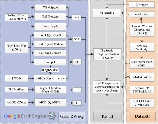
3.3. Technical Flowchart of this Study

The Land Cover Change (LCC), which is influenced by both climate change and human activity, usually affects wind erosion on surface roughness and soil physical and chemical characteristics. Therefore, we studied the SWEP of different land cover types and SWEP changes caused by the conversion of different land cover types. In this study, we chose ESA-CCI 300 m global land use land cover data products developed using the GlobCover unsupervised classification chain and by merging multiple available Earth observation products. Based on the United Nation Land Cover Classification System’s (LCCS) plant functional types (PET), the CCI-LC map is classified into 22 land types. According to the study area land characteristics, the land cover types are reclassified into nine categories based on the look-up table-conversion of CCI-LC classes to PET in the product user guide [81].
Based on the objective of this study, this manuscript is organized as presented in the technical flowchart (Figure 2). The research consists of four main steps: First, based on a time-series decomposition model, the wind speed variability of ground measurement data and reanalysis data was explored; second, by using multi-source geospatial data, the monthly SWEP across CA was generated based on GEE-RWEQ, and we explored the spatiotemporal variation of SWEP between 2000 and 2019; third, based on DSI and satellite-based AOD, validation was conducted to test the reliability of annual SWEP; and finally, we investigated the responses of wind erosion to ground measurement wind speed change and land cover change.
The ArcGIS10.6 software was implemented for land cover type reclassification in this research. The Pearson correlation coefficient (r) was calculated in R 3.6.3. The time-series decomposition model based on the “tseries” package was also run in R 3.6.3. The exponential fitting of the soil pH and soil calcium carbonate was performed in MATLAB 2018a.

4. Results, Analysis, and Validation

4.1. Variability of the Daily Average Wind Speed across CA

As the key factor of wind erosion, wind speed variability plays a vital role in wind erosion dynamics. A host of studies have reported that there was a declining trend in the global near-surface wind speed from 1970 to 2010 [14,17,18,19]. However, a recent study described an increase in the global wind speed during a particular year. Zeng, et al. [22] found that, after several decades of global terrestrial stilling, the wind speed has increased rapidly across the globe since 2010. Although Zeng, et al. [22] have investigated the global temporal variation of the wind speed, further studies are required because of the sensitivity of CA to global climate change [60].
To better understand the temporal variations of wind speed, it is possible to decompose wind speed time series data into sub-components by a time-series decomposition model. In this study, we used a multiplicative decomposition model, which is more effective when a seasonal value changes over time [82]. The calculation of this model included the following three steps [83]. The trend component was first determined and removed from time series by using the moving averages method. Secondly, the seasonal component was calculated and centered by averaging all periods for each time unit. In this study, a time-series decomposition multiplicative model was applied to Ground Measurement Wind Speed (GMWS) data. Figure 3 shows that the time series data were decomposed into various sub-components (the trend component, seasonal component, and random component). According to the trend component of the GMWS time series, we found that there was a significant decrease during the time period of 2000–2009 and a significant increase trend in the time period of 2009–2014. Moreover, GMWS exhibited steady fluctuations or a slight upward trend after 2014. From the perspective of quantitative analysis, we calculated the decade change rate of GMWS in these three time periods based on a linear regression analysis of ordinary least squares (OLS). The analysis shows that the daily average GMWS decreased significantly at a rate of −0.16 m s−1 decade−1 during the period of 2000–2009 (p < 0.001). After the turning point of 2009, the increasing rate of 0.42 m s−1 decade−1 was significantly higher than the decreasing rate during the period of 2009–2014 (p < 0.001). Although the GMWS shows a slight trend in recent years, the result is not statistically significant (p > 0.05). The time series of seasonal components indicated that the highest values for the daily average wind speed occurred during the spring, while the lowest values occurred during the autumn. The relationship between the daily average wind speed in different seasons is spring > winter > summer > autumn.
In order to ensure the consistency of the reanalysis data input by the model and the actual observation data in CA, the trends of four reanalysis data (GLDAS2.1, ERA5, CFSR, and FLDAS) were introduced to conduct comparisons with GMWS. The comparison result showed that the daily average derived from GLDAS2.1 has the highest correlation with the ground measurement wind speed (Supplementary Materials Figure S1). Furthermore, in order to better compare the relationship between the wind speed in trend and seasonal components, we decomposed the GLDAS2.1 wind speed time series into trend component, seasonal component, and random component. Additionally, we calculated the correlation coefficient (r) of the daily average wind speed and components between ground measurement data and reanalysis data. The trend component had the highest correlation coefficient (r = 0.829), followed by the seasonal component (r = 0.552), daily average wind speed (r = 0.125), and random component (r = −0.007). On the other hand, according to the trend component, the turning point for the GLDAS wind speed (GLDASWS) time series occurred around 2011 (Figure 4). Moreover, the changing rate of the daily average wind speed is more significant. The result of linear regression shows that the daily average GLDASWS decreased significantly at a rate of −0.34 m s−1 decade−1 during the period of 2000–2010 (p < 0.001). The increasing rate of 1 m s−1 decade−1 is significantly higher than the decreasing rate during the period of 2010–2014 (p < 0.001) after the turning point of 2010 (Figure 4). The seasonal components of two wind speed data have a broadly similar pattern.

4.2. The Spatiotemporal Variation of Wind Erosion across CA

Figure 5 shows the distribution of the annual mean SWEP in CA over the most recent 20 years (2000–2019). SWEP exhibits significant spatial variation, which has a range of 0–256 kg/m2. The SWEP in the southwest CA is higher than that in the southeast and north CA, where the vegetation coverage and soil moisture are higher. During the past 20 years, the Aral Sea dry lake bed (ASDLB), which is one of the most active dust sources, was the most severe wind erosion area in CA (47.29 kg/m2/y), followed by Kyzylkum Desert (10.64 kg/m2/y), Karakum Desert (10.58 kg/m2/y), and Muyunkum Desert (6.81 kg/m2/y). Due to the dramatic shrinkage of Aral Sea from the second half of the 20th century, the ASDLB, also known as the Aral Sea Desert, was covered with the original salts and chemicals of the water [24]. The toxic sediments of the Aral Sea were blown away by strong winds and formed white sandstorms. These toxic particles from the dry Aral Sea lake bed had been found in Japan, Norway, Greenland, and even in the South Pole [84].
From 2000 to 2019, the annual mean value of SWEP was 3.45 kg/m2, with the lowest value occurring in 2010 and the highest value occurring in 2015. As mentioned above, the wind speed exhibited a significant increase around 2011, and the area and intensity of wind erosion have also increased significantly since 2011. However, the SWEP gradually decreased by −6.85 kg/m2/y, over ASDLB, from 2011 (Figure 5). This reversal may have been caused by the recovery of the water body of the Aral Sea since 2010 [85]. This means that more dry lake beds are covered by water bodies and less bareland suffers from wind erosion. The Amu Darya River (ADR) and Syr Darya River (SDR), which are the two largest rivers across CA, are the principal water suppliers of the Aral Sea. Since the 1960s, many irrigation canals have been constructed in the middle and lower reaches of ADR and SDR [60]. Therefore, according to ESA land cover data, more than 43% of the irrigation cropland of CA survived on these canals, especially in Amu Darya Delta (ADD) and Syr Darya Delta (SDD). The main land cover type of these two deltas is irrigated cropland, which accounts for more than 20% of the total irrigated cropland in CA. Because of the high vegetation coverage, according to Figure 5, the ADD and SDD regions have a lower SWEP than the surrounded area. Similarly, on the edge of the Kyzylkum Desert, oasis agriculture that relies on irrigation also greatly reduces SWEP.
The seasonal variation characteristics of SWEP in CA are shown in Figure 6. Although it is usually consistent with the spatial distribution of the annual mean SWEP, the spatial pattern of SWEP varies in different seasons. As we can see in Figure 6, more land suffered from severe wind erosion in CA during the spring than in other seasons (spring: 1.48 kg/m2 > summer: 0.70 kg/m2 > winter: 0.69 kg/m2 > autumn: 0.59 kg/m2). Additionally, obvious wind erosion exists in several famous desert regions, such as the Karakum Desert, Kyzylkum Desert, and Aralkum Desert during spring. Due to the impact of snow cover, less wind erosion exists in north CA during the winter. However, the wind speed of the Aral region in winter markedly exceeds that in other seasons, especially in December. Therefore, the ASDLB region has higher SWEP in the winter. Figure 6 shows that the north Kazakhstan region, Kyrgyz, Tajikistan, has been slightly affected by wind erosion. Additionally, in summer, SWEP shows a significant high value in the middle reaches of Amu Darya (Figure 6). As shown in Figure 7, the SWEP displays significant monthly temporal variability, especially in ASDLB. March is the most severe month of wind erosion in the ASDLB. Alternatively, due to strong winds and dry surface soil in December, January, and February, sandstorms frequently occurred in ASDLB. We can confirm this from the true color image of MODIS (Supplementary Figure S2). Due to the difference in the solar radiation energy received by different latitudes, the melting time of snow cover varies in different regions. Figure 6 shows that the center of wind erosion moves from southwest to northeast during the spring (March, April, and May). These factors can explain why significant wind erosion in other famous deserts occurs in different months. The most severe month of wind erosion in Karakum is April, and that in Kyzylkum Desert and Muyunkum Desert is May. However, in general, Central Asia has suffered from the most severe wind erosion in April and the most widespread wind erosion in May.

4.3. Responses to Wind Speed Change and Land Cover Change

4.3.1. Impacts of Ground Measurement Wind Speed Changes on the SEWP

Based on the research results mentioned above, the wind speed was found to be the dominant factor of wind erosion. Therefore, in this study, we analyzed the influence of wind speed as a factor of climate change on wind erosion. Based on the ground measurement wind speed data, we investigated the influence of wind speed changes on wind erosion. Figure 8 shows the strong and significant positive correlation (r = 0.700, p < 0.001) between the average GMWS and average ground SWEP. According to the trend line of these two sets of time-series data, the turning point roughly occurred between 2010 and 2011. The average GMWS showed a slowly decreasing trend (−0.07 ms−1 decade−1) before the turning point in 2011, while it displayed a significant increasing trend during the period of 2011–2019 (+0.6 ms−1 decade−1, p < 0.001). The recent increasing rate is almost tenfold the decreasing rate in the first decade. The average ground SWEP also showed a slightly decreasing trend during the period of 2000–2010 (−0.027 kgm−2 decade−1), while it displayed a significant increasing trend (+0.37 kgm−2 decade−1, p < 0.001). Shao, et al. [86] found that the global monthly mean dust concentration decreased from 2000 to 2012. This shows that the end of the quiet period of dust activities in Central Asia or globally marks the beginning of an active period of dust activities. Based on current research, it seems reasonable to relate the dust trend to the climate trend, especially the reversal in global terrestrial stilling [22].
Additionally, the highest monthly average SWEP, which appeared in May 2014, was more than 2.4 kg/m2. The seven months with the strongest wind erosion (SWEP > 1.5 kg/m2) were March (2), April (2), May (2), and December (1). There were nine months (May: 3, March: 3, April: 2, Decembeer: 1) with an average wind speed greater than 3.5 m/s. Moreover, the highest monthly average wind speed, with a value of 3.79 m/s, appeared in Decembr 2015. Overall, a similar tendency of wind speed and wind erosion was observed for the past two decades. Both show a distinguishable declining trend, and then a sudden remarkable increase, and before slowly declining or finally stabilizing. During the study period, the wind speed (+0.38 ms−1 decade−1, p < 0.001) and SWEP (+0.34 kgm−2 decade−1, p < 0.001) increased very quickly from 2000 to 2019, indicating a more serious soil degradation and air pollution problem in CA.

4.3.2. Divergence of SWEP from Different Land Cover Types

According to the land characteristics of the study area, the ESA CCI land cover types can be reclassified into nine categories (cropland irrigated, cropland rain-fed, forestland, shrubland, grassland, sparse vegetation land, bareland, urbanland, and waterbody). The last subplot of Figure 9 shows the areas of different land cover types across CA in 2018. Figure 9 shows that the monthly average SWEP and its change rate of different land cover types were substantially different. The monthly average SWEP of bareland was more than 0.836 kg/m2, followed by shrubland (0.572 kg/m2), sparse vegetation land (0.203 kg/m2), grassland (0.073 kg/m2), irrigated cropland (0.043 kg/m2), rainfed cropland (0.033 kg/m2), and forestland (0.017 kg/m2). This relationship is basically consistent with previous research conducted in CA and surrounding regions [20,87]. We also compared the soil wind erosion modulus with respect to regions with similar conditions or the use of different methodologies (Table 2). Li, et al. [20] assessed the soil wind erosion modulus variation in CA (including Xinjiang, China) between 1986 and 2005. Zhang, et al. [87] investigated the RWEQ-based soil wind erosion, which was validated by 137Cs in Inner Mongolia (IM), during the time period of 1990–2015. Compared to other arid or semiarid regions, CA has relatively higher rates of soil wind erosion, which may be the result of the widespread distribution of deserts and wind speed increase in the past decade. Grassland has a relatively lower soil wind erosion rate, because it is mainly distributed in northern CA, which has a more humid climate and less erodible underlying surface condition [12]. Although the time periods and dataset sources were different, from the perspective of the wind erosion diversity of land cover, the wind erosion result of our research is reliable.
There was a significant increase in SWEP in CA in the past two decades. However, the change rate of wind erosion varied among regions with various types of land cover. Specifically, the change rate of wind erosion was the highest for bareland (0.0978 kg/m2/y), followed by shrubland (0.0730 kg/m2/y), sparse vegetation land (0.0206 kg/m2/y), grassland (0.0062 kg/m2/y), irrigated cropland (0.0045 kg/m2/y), rainfed cropland (0.0038 kg/m2/y), and forestland (0.0016 kg/m2/y). Combined with the areas of different land covers, we could calculate the total amount of soil wind loss for different land covers in the period of 2000–2019. More than 2.8255 × 10¹¹t soil was eroded by the wind across CA during the past few decades. The soil wind erosion of bareland (1.838 × 10¹¹t) contributed more than 65% soil loss by the wind in CA, followed by shrubland (0.3907 × 10¹¹t), sparse vegetation land (0.3380 × 10¹¹t), grassland (0.1812 × 10¹¹t), rainfed cropland (0.0517 × 10¹¹t), irrigated cropland (0.0223 × 10¹¹t), and forestland (0.0028 × 10¹¹t).
According to the continuous changes in the land cover area in CA during the period of 2000–2018, the cropland, forestland, urbanland, and shrubland showed an increased trend, while bareland and grassland showed a decreased trend (Supplementary Table S1). More than 2.67 × 10 km2 land had undergone land cover change, including from bareland to grassland, sparse vegetation land to grassland, grassland to cropland (rain-fed), sparse vegetation land to cropland (rain-fed), and waterbody to bareland. In order to remove wind speed variability effects on SWEP, we calculated the annual SWEP of 2018 based on the wind speed data of 2000 to compare it with the annual SWEP of 2000. We found that the LCCs with the strongest inhibitions of wind erosion activity were bareland into shrubland (−0.782 kg/m2), sparse vegetation land into forestland (−0.106 kg/m2), and grassland into forestland (−0.073 kg/m2). In comparison, the conversions of land cover which accelerated wind erosion the most were waterbody into bareland (+3.784 kg/m2), sparse vegetation land into bareland (+1.124 kg/m2), and grassland into bareland (+0.490 kg/m2).

4.4. Validation of the GEE-RWEQ Model

Due to lack of long time series and wide range of ground-measured wind erosion data in CA, validation of the GEE-RWEQ model is challenging. Furthermore, due to the large area and complex terrain conditions, almost no previous research has conducted wind erosion field measurements in CA. Considering that most of the local dust storms are caused by surface wind erosion in CA [24], the dust storm index (DSI) can be used as a proxy to evaluate the wind erosion model performance [75]. Therefore, we used the DSI based on weather station visibility records to evaluate the reliability of the SWEP spatial distribution. Figure 10 displays the annual mean DSI across CA from 2000 to 2019. This map was interpolated by the annual average DSI of more than 200 weather stations based on Natural Neighbor Interpolation method. From Figure 10, we can see that the southwest desert region of CA has a high DSI, which means very frequent dust storms. However, there are some high values in the southeastern parts of CA, where there is a lower wind erosion risk. According to the research of Liu, et al. [89], affected by the strong southwest winds, the dust particles were transported from the western desert to eastern mountains and valley. Moreover, dust episodes were observed in these regions. Additionally, the southeastern parts of CA are the most densely populated areas in CA. Most of the weather stations across CA are located around densely populated cities. The anthropogenic pollutants will also be recognized as dusty weather due to reduced visibility. The spatial distribution of DSI is generally consistent with the spatial pattern of the annual SWEP. Although visibility records based on weather stations are a valuable and useful data resource for wind erosion monitoring, several limitations still exist. The low spatial density of weather stations is a challenge for conducting highly accurate wind erosion mapping, especially in the southeastern part of CA. Therefore, we need to obtain higher spatial resolution and more continuous SWEP verification data. It should be pointed out that satellite-based atmospheric aerosols, which refer to solid and liquid particles suspended in the atmosphere, have strong spatial correlations with wind erosion.
Figure 11 shows the spatial pattern of the annual AOD (a) and average AAI in 2019 (b), as well as the comparisons with SWEP in the Aral Sea region (ASR). From Figure 11, we can see that the Aral Sea region and its southwest surrounding area has the highest value in CA. This is because the dust of the Aral Sea is transported to the southwest under the action of the dominant wind-northeast wind [90]. Therefore, we chose ASDLB as a research hotspot area to compare with SWEP. Linear relationships between SWEP and aerosol parameters (AOD and AAI) were found, as shown in Figure 11. The results show that they had moderate positive linear relationships, with r values of 0.5623 (p < 0.001) and 0.5660 (p < 0.001), respectively. Ultimately, although it is difficult to verify the SWEP value, the comparison results obtained from the perspective of spatial and temporal distribution patterns showed that the RWEQ-based SWEP data in CA were reliable.

5. Discussion

In this study, our results show that there are significant spatial and temporal differences in the wind erosion in CA. Controlled by the latitude zonality and vertical zonality, higher SWEP values are primarily distributed in the southwestern part of CA, which has low vegetation coverage and more fragile surface soil [91], while lower SWEP is mainly concentrated in the northern part of CA. Based on the land cover map of 2018, more than 89% of rain-fed cropland and 78% of forestland are distributed in these regions. Furthermore, due to latitude zonality and vertical zonality, the precipitation in these areas is higher than in other places of CA, and the temperatures in these areas are lower. Therefore, the higher soil moisture caused by lower evapotranspiration will reduce the wind erosion to a certain degree. Affected by the restoration of the Aral Sea in recent years, the vegetation coverage and other underlying surface factors of ASDLB are getting better [85]. Although the SWEP showed a decreasing trend in ASDLB (−6.85 kg/m2/y), this region was still the most severe wind erosion area in CA. In addition, our results show that the SWEP has a clear seasonal and monthly variation. The land threatened by wind erosion has the largest range in spring, especially in May. Due to the difference in solar radiation heat at different latitudes and altitudes, the snowmelt period varies in different regions of CA [92]. The higher soil moisture caused by snowmelt and the snow cover both affected the movement of the wind erosion center across CA during spring [37]. Therefore, considering the major deserts of CA are located in different latitudes and altitudes, the severe wind erosion regions in CA will also migrate over time. The severe wind erosion regions move from the southwest CA (Karakum Desert) to the middle CA (Kyzylkum Desert and Muyunkum Desert) during the spring (MAM). However, due to the special meteorological conditions in certain areas of CA, such as the middle reaches of the ADR, severe wind erosion occurs in summer, but not spring, respectively [24]. We calculated the monthly average wind speed of four weather stations in this region. A comparison was made for the monthly average wind speed of all the weather stations in CA and the four weather stations in this region (Supplementary Figure S3). The most extreme value of the surface wind speed in CA appeared in March, while the most extreme value of the wind speed in the middle reaches of the ADR appeared in July. This result demonstrates that wind speed plays the key role in the spatial distribution of SWEP.
As the most dominant factors of wind erosion, wind speed variability, such as wind stilling or wind stilling reversal, account for the majority of the spatial-temporal variation of wind erosion in CA. Although global terrestrial stilling has been confirmed by many pieces of research, most studies have only looked at global or regional wind speed changes from the 1980s to 2010, and few have involved recent (after 2010) wind speed changes [14,17,18,19]. According to several climate assimilation datasets (GLDAS, ERA5, CFSR, and FLDAS) and a ground measurement dataset (GSOD), we found a turning point of wind speed stilling during the period of 2009–2012 in CA. This finding is supported by other studies that have reported that global terrestrial stilling has rebounded over the past few decades and has increased rapidly since 2010 [21,22,23]. Our research proves that the increase rate of the average wind speed in CA (0.6 m s−1 decade−1) is higher than the increase rate of the average global wind speed (0.24 m s−1 decade−1) over the same period, which means that stronger wind erosion occurred in CA. Indeed, the result shows a strong and significant positive correlation (r = 0.7) between the average GMWS and average SWEP (p < 0.001). A number of studies have demonstrated that CA is more sensitive to climate change compared to the global average [12,20,57,60,91,93]. While it is widely acknowledged that the global wind speed rebound is beneficial to the wind power industry for the near future [22], this study suggests that more severe wind erosion activity happened in CA.
According to the significant differences in natural conditions, such as the air temperature and precipitation, and the disturbance of human activities such as irrigation, the land cover in CA exhibited strong spatial differentiation. We found that SWEP differs greatly in different land cover types. This result is roughly consistent with a previous study on wind erosion in CA and surrounding regions [20,87]. Most of the shrubland in CA is made up of deserts and xeric shrublands in which Haloxylon ammodendron, Calligonum aphyllum, and Ephedra lomatolepis, as well as grasses such as Agropyron fragile, grow [94,95,96]. These kinds of vegetation have good windproof and sand fixing functions in CA. In addition, LCCs are closely related to wind erosion activity and affect each other. From 2000 to 2018, more than 2.6 × 10⁵ km2 of land has changed land cover types (Supplementary Table S1). We compared the SWEP for the land with the LCC from 2000 to 2018, in which the effect of the wind speed variability was removed. The conversion of bareland to shrubland helped reduce wind erosion by −0.782 kg/m2/y. Furthermore, due to the shrinkage of the Aral Sea, the conversion of waterbody to bareland increased wind erosion by +3.784 kg/m2/y. The restoration of the Aral Sea has not only superficially reduced the possibility of wind erosion in ASDLB, but also increased the increased vegetation coverage of ASDLB caused by the higher groundwater level, making the long-distance transport of dust difficult. Although the wind speed has shown an increasing trend in the past 10 years, the wind erosion risk in the Aral Sea area is gradually decreasing due to the continuous recovery of the Aral Sea area. In the past 30 years, a large number of engineering projects have attempted to improve the Aral Sea environment, directly or indirectly. Although Aral sea restoration is the most effective way to restrain wind erosion in ASDLB, the complex political relations among countries in the Aral Sea basin make cross-border water management difficult [84]. Besides, in other parts of CA, more effective measures should be taken for wind erosion artificial control, for example, increasing the grassland area in regions with a suitable temperature and precipitation, developing cropland by using limited water resources, and planting cold- and drought-resistant shrub vegetation in bareland.
In this study, the RWEQ model was adopted as a wind erosion model in the GEE cloud computing platform. Compared with the local computing platform, GEE can process large amounts of geospatial data in a short time, which means that its processing power is completely unconstrained by time and space. Therefore, we do not need to spend a lot of time on downloading, preprocessing, and model running of a large amount geo-spatial data, which can greatly shorten the time required for long-term wind erosion mapping. As mentioned above, GEE-RWEQ provides the possibility of wind erosion monitoring in developing regions lacking on-site monitoring data. Meanwhile, the GEE platform makes it easier for researchers to publish their results for decision makers, and even the public [55]. Therefore, our research has a broader application value for decision makers than previous studies on wind erosion. In the future, we will interactively develop Earth Engine App to explore our result, which can then be used by experts and non-experts alike.
The RWEQ is a process-based, field-scale, empirical model that can quantitatively estimate wind erosion. However, the RWEQ was initially developed for the middle western area of the United States [37]. Therefore, it still presents some limitations in other regions [37,50,72,97]. Although the most important input parameters were retained in this study, the dataset required by some parameters was unavailable on GEE platforms. Therefore, several factors were simplified to simulate the global-scale wind erosion more effectively and more accurately. The soil moisture data were used to simulate how the surface wetness influences the wind speed required to erode the soil. Additionally, the cosine of the slope gradient which was calculated by DEM represented the soil roughness factor. On the other hand, we only used wind erosion-related data such as visibility data and remote sensing data for the verification of wind erosion in CA, but this still has uncertainties on a global scale. Central Asia, which is one of the most severe wind erosion regions, is restricted in terms of wind erosion modeling studies due to the lack of wind erosion measurement data for this region. Therefore, more ground soil loss measurement data on a global scale should be acquired to conduct more verification studies.

6. Conclusions

In this study, we developed a fully automated algorithm for quantitatively mapping wind erosion based on the Google Earth Engine, processed terabytes of geo-spatial data, and retrieved spatial and temporal patterns of monthly SWEP in CA, over 20 years (2000 to 2019). Several conclusions were reached in our study, as follows:
(1) With respect to the conventional methods, GEE-RWEQ does not require any ground measurement data, which need lots of manpower and resources, especially in developing countries or sparsely populated regions. However, based on the Cloud computing platform, GEE-RWEQ uses climate assimilation data, soil property data, vegetation data, terrain data, and other underlying data to automatically generate high spatial resolution NRT soil wind erosion potential products. After verification using ground observation-based DSI and satellite-based AOD, the results still reach an acceptable accuracy and can be used for quantitative wind erosion mapping. This methodology provides new ideas for the construction and use of empirical models based on batch geospatial data and high-performance computing;
(2) According to the comparison of GMMS and SWEP, the wind speed is the main driving factor of wind erosion (r = 0.7, p < 0.001). Affected by the wind speed variability, the SWEP decreased first and increased remarkably during 2011. From the perspective of the temporal and spatial distribution, due to the sparse vegetation distribution and special meteorological conditions, the deserts in southwestern Central Asia are most affected by wind erosion, especially in ASDLB (47.29 kg/m2/y). The severe wind erosion period of CA occurred in spring (MAM), especially in May. We also found that the SWEP distribution has obvious latitude zonality due to the distribution of snow cover and the start time of snow melt, and the wind erosion hot spot in spring moves from the southwest to central area across CA;
(3) Land cover change has strong effects on the soil wind erosion in CA, with the most obvious being the conversion of bareland into the water body in ASDLB. Affected by the restoration of the Aral Sea, the SWEP in this area has shown a downward trend (−6.85 kg/m2/y) since 2011. Additionally, the conversion of bareland to shrubland helped reduce wind erosion by −0.782 kg/m2/y. According to the SWEP variation based on LCC, more effective measures should be taken to maintain wind erosion artificial control, for example, restoring the Aral Sea water area to prevent more bareland from being exposed to wind erosion, increasing the grassland area in regions with a suitable temperature and precipitation, developing cropland by using limited water resources, and planting cold- and drought-resistant shrub vegetation in bareland.

Supplementary Materials

The following are available online at https://www.mdpi.com/2072-4292/12/20/3430/s1, Figure S1: Comparisons of the wind speed trend for different datasets (FLDAS, CFSR, ERA5, GLDAS2.1, and GMMS); Figure S2: Dust events in the Aral Sea during winter captured by MODIS; Figure S3: Monthly average wind speed of CA and the other four weather stations in the middle reaches of Amu Darya; and Table S1: The areas of different land cover types in Central Asia during the period of 2000–2018.

Author Contributions

Conceptualization, W.W.; data curation, W.W., Y.G., and A.T.; formal analysis, W.W. and Y.G.; funding acquisition, J.A.; methodology, W.W. and A.S.; project administration, A.S. and L.M.; resources, A.S. and J.A.; software, W.W. and S.Z.; supervision, J.A.; writing—original draft, W.W.; writing—review and editing, W.W. and A.S. All authors have read and agree to the published version of the manuscript.

Funding

This research was funded by the Strategic Priority Research Program of the Chinese Academy of Sciences, grant number XDA20060301; by the Youth Innovation Promotion Association Foundation of the Chinese Academy of Sciences under Grant 2018476; and in part by the National Natural Science Foundation of China, grant number 42071424.

Acknowledgments

The authors would like to give special thanks to the Google Earth Engine team for their support and allowing access. We appreciate the FLDAS, CFSR, ERA5, GLDAS, MODIS, Sentinel5P, and OLM soil properties data made available via the GEE. We are grateful for meteorological station data provided by the National Oceanic and Atmospheric Administration (NOAA). The GEE JavaScript code for retrieving SWEP can be made available by contacting the first author.

Conflicts of Interest

The authors declare no conflict of interest.

References

  1. Borrelli, P.; Robinson, D.A.; Fleischer, L.R.; Lugato, E.; Ballabio, C.; Alewell, C.; Meusburger, K.; Modugno, S.; Schütt, B.; Ferro, V.; et al. An assessment of the global impact of 21st century land use change on soil erosion. Nat. Commun. 2017, 8, 2013. [Google Scholar] [CrossRef] [Green Version]
  2. Chasek, P.; Akhtar-Schuster, M.; Orr, B.J.; Luise, A.; Rakoto Ratsimba, H.; Safriel, U. Land degradation neutrality: The science-policy interface from the UNCCD to national implementation. Environ. Sci. Policy 2019, 92, 182–190. [Google Scholar] [CrossRef]
  3. Borrelli, P.; Robinson, D.A.; Panagos, P.; Lugato, E.; Yang, J.E.; Alewell, C.; Wuepper, D.; Montanarella, L.; Ballabio, C. Land use and climate change impacts on global soil erosion by water (2015–2070). Proc. Natl. Acad. Sci. USA 2020, 117, 21994. [Google Scholar] [CrossRef] [PubMed]
  4. Oldeman, L. The Global Extent of Soil Degradation; ISRIC: Wageningen, The Netherlands, 1994; pp. 19–36. [Google Scholar]
  5. Lal, R. Soil degradation and global food security: A soil science perspective. In Land Quality, Agricultural Productivity, and Food Security: Biophysical Processes and Economic Choices at Local, Regional, and Global Levels; Wiebe, K., Ed.; Edward Elgar Publishing: London, UK, 2003; pp. 16–35. [Google Scholar]
  6. UNCCD. What is Desertification? Available online: https://www.unccd.int/frequently-asked-questions-faq (accessed on 21 July 2020).
  7. Pimentel, D.; Burgess, M. Soil Erosion Threatens Food Production. Agriculture 2013, 3, 443–463. [Google Scholar] [CrossRef] [Green Version]
  8. Joint Research Centre; European Soil Data Centre. Wind Erosion. Available online: https://esdac.jrc.ec.europa.eu/themes/wind-erosion (accessed on 21 July 2020).
  9. Duniway, M.C.; Pfennigwerth, A.A.; Fick, S.E.; Nauman, T.W.; Belnap, J.; Barger, N.N. Wind erosion and dust from US drylands: A review of causes, consequences, and solutions in a changing world. Ecosphere 2019, 10, e02650. [Google Scholar] [CrossRef] [Green Version]
  10. Jiang, C.; Liu, J.; Zhang, H.; Zhang, Z.; Wang, D. China’s progress towards sustainable land degradation control: Insights from the northwest arid regions. Ecol. Eng. 2019, 127, 75–87. [Google Scholar] [CrossRef]
  11. Rashki, A.; Eriksson, P.G.; Rautenbach, C.J.d.W.; Kaskaoutis, D.G.; Grote, W.; Dykstra, J. Assessment of chemical and mineralogical characteristics of airborne dust in the Sistan region, Iran. Chemosphere 2013, 90, 227–236. [Google Scholar] [CrossRef] [Green Version]
  12. Jiang, L.; Jiapaer, G.; Bao, A.; Kurban, A.; Guo, H.; Zheng, G.; De Maeyer, P. Monitoring the long-term desertification process and assessing the relative roles of its drivers in Central Asia. Ecol. Indic. 2019, 104, 195–208. [Google Scholar] [CrossRef]
  13. Shen, H.; Abuduwaili, J.; Samat, A.; Ma, L. A review on the research of modern aeolian dust in Central Asia. Arab. J. Geosci. 2016, 9, 625. [Google Scholar] [CrossRef]
  14. Zhang, G.; Azorin-Molina, C.; Shi, P.; Lin, D.; Guijarro, J.A.; Kong, F.; Chen, D. Impact of near-surface wind speed variability on wind erosion in the eastern agro-pastoral transitional zone of Northern China, 1982–2016. Agric. For. Meteorol. 2019, 271, 102–115. [Google Scholar] [CrossRef]
  15. Qi, J.; Kulmatov, R. An Overview of Environmental Issues in Central Asia. In Proceedings of Environmental Problems of Central Asia and their Economic, Social and Security Impacts; Springer: Dordrecht, The Netherlands, 2008; pp. 3–14. [Google Scholar]
  16. Ge, Y.; Abuduwaili, J.; Ma, L. Lakes in Arid Land and Saline Dust Storms. E3s Web Conf. 2019, 99, 01007. [Google Scholar] [CrossRef]
  17. Guo, H.; Xu, M.; Hu, Q. Changes in near-surface wind speed in China: 1969–2005. Int. J. Climatol. 2011, 31, 349–358. [Google Scholar] [CrossRef]
  18. Azorin-Molina, C.; Rehman, S.; Guijarro, J.A.; McVicar, T.R.; Minola, L.; Chen, D.; Vicente-Serrano, S.M. Recent trends in wind speed across Saudi Arabia, 1978–2013: A break in the stilling. Int. J. Climatol. 2018, 38, e966–e984. [Google Scholar] [CrossRef]
  19. McVicar, T.R.; Van Niel, T.G.; Li, L.T.; Roderick, M.L.; Rayner, D.P.; Ricciardulli, L.; Donohue, R.J. Wind speed climatology and trends for Australia, 1975–2006: Capturing the stilling phenomenon and comparison with near-surface reanalysis output. Geophys. Res. Lett. 2008, 35. [Google Scholar] [CrossRef] [Green Version]
  20. Li, J.; Ma, X.; Zhang, C. Predicting the spatiotemporal variation in soil wind erosion across Central Asia in response to climate change in the 21st century. Sci. Total Environ. 2020, 709, 136060. [Google Scholar] [CrossRef] [PubMed]
  21. Kim, J.; Paik, K. Recent recovery of surface wind speed after decadal decrease: A focus on South Korea. Clim. Dyn. 2015, 45, 1699–1712. [Google Scholar] [CrossRef]
  22. Zeng, Z.; Ziegler, A.D.; Searchinger, T.; Yang, L.; Chen, A.; Ju, K.; Piao, S.; Li, L.Z.X.; Ciais, P.; Chen, D.; et al. A reversal in global terrestrial stilling and its implications for wind energy production. Nat. Clim. Chang. 2019, 9, 979–985. [Google Scholar] [CrossRef]
  23. Azorin-Molina, C.; Menendez, M.; McVicar, T.R.; Acevedo, A.; Vicente-Serrano, S.M.; Cuevas, E.; Minola, L.; Chen, D. Wind speed variability over the Canary Islands, 1948–2014: Focusing on trend differences at the land-ocean interface and below–above the trade-wind inversion layer. Clim. Dyn. 2018, 50, 4061–4081. [Google Scholar] [CrossRef] [Green Version]
  24. Issanova, G.; Abuduwaili, J. Relationship between Storms and Land Degradation. In Aeolian Proceses as Dust Storms in the Deserts of Central Asia and Kazakhstan; Issanova, G., Abuduwaili, J., Eds.; Springer: Singapore, 2017; pp. 71–86. [Google Scholar] [CrossRef]
  25. Pi, H.; Sharratt, B.; Lei, J. Wind erosion and dust emissions in central Asia: Spatiotemporal simulations in a typical dust year. Earth Surf. Process. Landf. 2019, 44, 521–534. [Google Scholar] [CrossRef]
  26. Chappell, A.; Webb, N.P.; Guerschman, J.P.; Thomas, D.T.; Mata, G.; Handcock, R.N.; Leys, J.F.; Butler, H.J. Improving ground cover monitoring for wind erosion assessment using MODIS BRDF parameters. Remote Sens. Environ. 2018, 204, 756–768. [Google Scholar] [CrossRef]
  27. Chappell, A.; Webb, N.P.; Leys, J.F.; Waters, C.M.; Orgill, S.; Eyres, M.J. Minimising soil organic carbon erosion by wind is critical for land degradation neutrality. Environ. Sci. Policy 2019, 93, 43–52. [Google Scholar] [CrossRef]
  28. Okin, G.S.; Gillette, D.A. Distribution of vegetation in wind-dominated landscapes: Implications for wind erosion modeling and landscape processes. J. Geophys. Res. Atmos. 2001, 106, 9673–9683. [Google Scholar] [CrossRef]
  29. Van Pelt, R.S.; Hushmurodov, S.X.; Baumhardt, R.L.; Chappell, A.; Nearing, M.A.; Polyakov, V.O.; Strack, J.E. The reduction of partitioned wind and water erosion by conservation agriculture. Catena 2017, 148, 160–167. [Google Scholar] [CrossRef]
  30. Du, H.; Zuo, X.; Li, S.; Wang, T.; Xue, X. Wind erosion changes induced by different grazing intensities in the desert steppe, Northern China. Agric. Ecosyst. Environ. 2019, 274, 1–13. [Google Scholar] [CrossRef]
  31. Shao, Y.; Leslie, L.M. Wind erosion prediction over the Australian continent. J. Geophys. Res. Atmos. 1997, 102, 30091–30105. [Google Scholar] [CrossRef] [Green Version]
  32. Hu, Y.; Liu, J.; Zhuang, D.; Cao, H.; Yan, H.; Yang, F. Distribution characteristics of 137Cs in wind-eroded soil profile and its use in estimating wind erosion modulus. Chin. Sci. Bull. 2005, 50, 1155–1159. [Google Scholar] [CrossRef]
  33. Zhang, C.-L.; Zou, X.-Y.; Yang, P.; Dong, Y.-X.; Li, S.; Wei, X.-H.; Yang, S.; Pan, X.-H. Wind tunnel test and 137Cs tracing study on wind erosion of several soils in Tibet. Soil Tillage Res. 2007, 94, 269–282. [Google Scholar] [CrossRef]
  34. Shao, Y. Integrated Wind-Erosion Modelling. In Physics and Modelling of Wind Erosion; Springer: Dordrecht, The Netherlands, 2008; pp. 303–360. [Google Scholar] [CrossRef]
  35. Williams, J.; Nearing, M.; Nicks, A.; Skidmore, E.; Valentin, C.; King, K.; Savabi, R. Using soil erosion models for global change studies. J. Soil Water Conserv. 1996, 51, 381–385. [Google Scholar]
  36. Fryrear, D.; Sutherland, P.; Davis, G.; Hardee, G.; Dollar, M. Wind erosion estimates with RWEQ and WEQ. In Proceedings of the 10th International Soil Conservation Organization Meeting; Purdue University and USDA-ARS National Soil Erosion Research Laboratory: West Lafayette, IN, USA, 2001; pp. 760–765. [Google Scholar]
  37. Fryrear, D.W.; Bilbro, J.D.; Saleh, A.; Schomberg, H.; Stout, J.E.; Zobeck, T.M. RWEQ: Improved wind erosion technology. J. Soil Water Conserv. 2000, 55, 183. [Google Scholar]
  38. Bagnold, R.A. The Physics of Blown Sand and Desert Dunes; William Morrow & Company: New York, NY, USA, 1941. [Google Scholar]
  39. Woodruff, N.P.; Siddoway, F.H. A Wind Erosion Equation. Soil Sci. Soc. Am. J. 1965, 29, 602–608. [Google Scholar] [CrossRef]
  40. Tatarko, J.; Sporcic, M.A.; Skidmore, E.L. A history of wind erosion prediction models in the United States Department of Agriculture prior to the Wind Erosion Prediction System. Aeolian Res. 2013, 10, 3–8. [Google Scholar] [CrossRef]
  41. Feng, G.; Sharratt, B. Evaluation of the SWEEP model during high winds on the Columbia Plateau. Earth Surf. Process. Landf. 2009, 34, 1461–1468. [Google Scholar] [CrossRef]
  42. Cole, G.W.; Lyles, L.; Hagen, L.J. A Simulation Model of Daily Wind Erosion Soil Loss. Trans. ASAE 1983, 26, 1758–1765. [Google Scholar] [CrossRef]
  43. Pi, H.; Sharratt, B.; Feng, G.; Lei, J. Evaluation of two empirical wind erosion models in arid and semi-arid regions of China and the USA. Environ. Model. Softw. 2017, 91, 28–46. [Google Scholar] [CrossRef] [Green Version]
  44. Gregory, J.M.; Wilson, G.R.; Singh, U.B.; Darwish, M.M. TEAM: Integrated, process-based wind-erosion model. Environ. Model. Softw. 2004, 19, 205–215. [Google Scholar] [CrossRef]
  45. Böhner, J.; Schäfer, W.; Conrad, O.; Gross, J.; Ringeler, A. The WEELS model: Methods, results and limitations. Catena 2003, 52, 289–308. [Google Scholar] [CrossRef]
  46. Zobeck, T.M.; Parker, N.C.; Haskell, S.; Guoding, K. Scaling up from field to region for wind erosion prediction using a field-scale wind erosion model and GIS. Agric. Ecosyst. Environ. 2000, 82, 247–259. [Google Scholar] [CrossRef]
  47. Chi, W.; Zhao, Y.; Kuang, W.; He, H. Impacts of anthropogenic land use/cover changes on soil wind erosion in China. Sci. Total Environ. 2019, 668, 204–215. [Google Scholar] [CrossRef]
  48. Borrelli, P.; Lugato, E.; Montanarella, L.; Panagos, P. A New Assessment of Soil Loss due to Wind Erosion in European Agricultural Soils Using a Quantitative Spatially Distributed Modelling Approach. Land Degrad. Dev. 2017, 28, 335–344. [Google Scholar] [CrossRef] [Green Version]
  49. Borrelli, P.; Panagos, P.; Ballabio, C.; Lugato, E.; Weynants, M.; Montanarella, L. Towards a Pan-European Assessment of Land Susceptibility to Wind Erosion. Land Degrad. Dev. 2016, 27, 1093–1105. [Google Scholar] [CrossRef]
  50. Lin, J.; Guan, Q.; Pan, N.; Zhao, R.; Yang, L.; Xu, C. Spatiotemporal Variations and Driving Factors of the Potential Wind Erosion Rate in the Hexi Region. Land Degrad. Dev. 2020. [Google Scholar] [CrossRef]
  51. Gorelick, N.; Hancher, M.; Dixon, M.; Ilyushchenko, S.; Thau, D.; Moore, R. Google Earth Engine: Planetary-scale geospatial analysis for everyone. Remote Sens. Environ. 2017, 202, 18–27. [Google Scholar] [CrossRef]
  52. Mutanga, O.; Kumar, L. Google Earth Engine Applications. Remote Sens. 2019, 11, 591. [Google Scholar] [CrossRef] [Green Version]
  53. Ivushkin, K.; Bartholomeus, H.; Bregt, A.K.; Pulatov, A.; Kempen, B.; de Sousa, L. Global mapping of soil salinity change. Remote Sens. Environ. 2019, 231, 111260. [Google Scholar] [CrossRef]
  54. Pradhan, B.; Moneir, A.A.A.; Jena, R. Sand dune risk assessment in Sabha region, Libya using Landsat 8, MODIS, and Google Earth Engine images. Geomat. Nat. Hazards Risk 2018, 9, 1280–1305. [Google Scholar] [CrossRef] [Green Version]
  55. Jin, Y.; Liu, X.; Yao, J.; Zhang, X.; Zhang, H. Mapping the annual dynamics of cultivated land in typical area of the Middle-lower Yangtze plain using long time-series of Landsat images based on Google Earth Engine. Int. J. Remote Sens. 2020, 41, 1625–1644. [Google Scholar] [CrossRef]
  56. Xie, Z.; Phinn, S.R.; Game, E.T.; Pannell, D.J.; Hobbs, R.J.; Briggs, P.R.; Beutel, T.S.; Holloway, C.; McDonald-Madden, E. Using Landsat observations (1988–2017) and Google Earth Engine to detect vegetation cover changes in rangelands—A first step towards identifying degraded lands for conservation. Remote Sens. Environ. 2019, 232, 111317. [Google Scholar] [CrossRef]
  57. Chen, Y.; Li, W.; Deng, H.; Fang, G.; Li, Z. Changes in Central Asia’s Water Tower: Past, Present and Future. Sci. Rep. 2016, 6, 39364. [Google Scholar] [CrossRef] [PubMed] [Green Version]
  58. Groll, M.; Opp, C.; Issanova, G.; Vereshagina, N.; Semenov, O. Physical and Chemical Characterization of Dust Deposited in the Turan Lowland (Central Asia). Proc. E3S Web Conf. 2019, 99, 03005. [Google Scholar] [CrossRef]
  59. Micklin, P. The Aral Sea Crisis. In Dying and Dead Seas Climatic Versus Anthropic Causes; Springer: Dordrecht, The Netherlands, 2004; pp. 99–123. [Google Scholar]
  60. Abuduwaili, J.; Issanova, G.; Saparov, G. Water Resources and Impact of Climate Change on Water Resources in Central Asia. In Hydrology and Limnology of Central Asia; Abuduwaili, J., Issanova, G., Saparov, G., Eds.; Springer: Singapore, 2019; pp. 1–9. [Google Scholar] [CrossRef]
  61. Rodell, M.; Houser, P.; Jambor, U.E.A.; Gottschalck, J.; Mitchell, K.; Meng, J.; Arsenault, K.; Brian, C.; Radakovich, J.; Mg, B.; et al. The Global Land Data Assimilation System. BAMS 2004, 85, 381–394. [Google Scholar] [CrossRef] [Green Version]
  62. Huang, D.K.; Xin-Qing, L.; Wei, J.; Zhao, Y.L.; Wen, C.; Ding, W. Geographic variation of carbonate content and pH in surface soil in East Central Asia: Significance as climate proxies. Geochimica 2008, 37, 129–138. [Google Scholar]
  63. Liu, S.; Zhang, S.; Wu, J.; Pang, X.; Yuan, D. The relationship between soil pH and calcium carbonate content. Soil 2002, 5. [Google Scholar] [CrossRef]
  64. Symeonakis, E.; Drake, N. Monitoring desertification and land degradation over sub-Saharan Africa. Int. J. Remote Sens. 2004, 25, 573–592. [Google Scholar] [CrossRef]
  65. Fenta, A.A.; Tsunekawa, A.; Haregeweyn, N.; Poesen, J.; Tsubo, M.; Borrelli, P.; Panagos, P.; Vanmaercke, M.; Broeckx, J.; Yasuda, H.; et al. Land susceptibility to water and wind erosion risks in the East Africa region. Sci. Total Environ. 2020, 703, 135016. [Google Scholar] [CrossRef]
  66. Naumann, G.; Barbosa, P.; Carrao, H.; Singleton, A.; Vogt, J. Monitoring Drought Conditions and Their Uncertainties in Africa Using TRMM Data. J. Appl. Meteorol. Climatol. 2012, 51, 1867–1874. [Google Scholar] [CrossRef] [Green Version]
  67. Kalantari, Z.; Ferreira, C.S.S.; Keesstra, S.; Destouni, G. Nature-based solutions for flood-drought risk mitigation in vulnerable urbanizing parts of East-Africa. Curr. Opin. Environ. Sci. Health 2018, 5, 73–78. [Google Scholar] [CrossRef]
  68. Ouyang, Z.; Zheng, H.; Xiao, Y.; Polasky, S.; Liu, J.; Xu, W.; Wang, Q.; Zhang, L.; Xiao, Y.; Rao, E.; et al. Improvements in ecosystem services from investments in natural capital. Science 2016, 352, 1455. [Google Scholar] [CrossRef] [PubMed]
  69. Wang, L.-Y.; Xiao, Y.; Rao, E.-M.; Jiang, L.; Xiao, Y.; Ouyang, Z.-Y. An Assessment of the Impact of Urbanization on Soil Erosion in Inner Mongolia. Int. J. Environ. Res. Public Health 2018, 15, 550. [Google Scholar] [CrossRef] [Green Version]
  70. Xu, J.; Xiao, Y.; Xie, G.; Wang, Y.; Jiang, Y. Computing payments for wind erosion prevention service incorporating ecosystem services flow and regional disparity in Yanchi County. Sci. Total Environ. 2019, 674, 563–579. [Google Scholar] [CrossRef] [PubMed]
  71. Zhang, J.; Li, X.; Buyantuev, A.; Bao, T.; Zhang, X. How Do Trade-Offs and Synergies between Ecosystem Services Change in the Long Period? The Case Study of Uxin, Inner Mongolia, China. Sustainability 2019, 11, 6041. [Google Scholar] [CrossRef] [Green Version]
  72. Jiang, L.; Xiao, Y.; Zheng, H.; Ouyang, Z. Spatio-temporal variation of wind erosion in Inner Mongolia of China between 2001 and 2010. Chin. Geogr. Sci. 2016, 26, 155–164. [Google Scholar] [CrossRef] [Green Version]
  73. Wu, D.; Zou, C.; Cao, W.; Xiao, T.; Gong, G. Ecosystem services changes between 2000 and 2015 in the Loess Plateau, China: A response to ecological restoration. PLoS ONE 2019, 14, e0209483. [Google Scholar] [CrossRef] [PubMed] [Green Version]
  74. McTainsh, G.H. Sustainable Agriculture: Assessing Australia’s Recent Performance. A Report of the National Collaborative Project on Indicators for Sustainable Agriculture; CSIRO: Canberra, Australia, 1998; pp. 65–72.
  75. O’Loingsigh, T.; McTainsh, G.H.; Tews, E.K.; Strong, C.L.; Leys, J.F.; Shinkfield, P.; Tapper, N.J. The Dust Storm Index (DSI): A method for monitoring broadscale wind erosion using meteorological records. Aeolian Res. 2014, 12, 29–40. [Google Scholar] [CrossRef]
  76. Lim, J.-Y.; Chun, Y. The characteristics of Asian dust events in Northeast Asia during the springtime from 1993 to 2004. Glob. Planet. Chang. 2006, 52, 231–247. [Google Scholar] [CrossRef]
  77. Wang, D.; Zhang, F.; Yang, S.; Xia, N.; Ariken, M. Exploring the spatial-temporal characteristics of the aerosol optical depth (AOD) in Central Asia based on the moderate resolution imaging spectroradiometer (MODIS). Environ. Monit. Assess. 2020, 192, 383. [Google Scholar] [CrossRef]
  78. Qin, W.; Wang, L.; Lin, A.; Zhang, M.; Bilal, M. Improving the Estimation of Daily Aerosol Optical Depth and Aerosol Radiative Effect Using an Optimized Artificial Neural Network. Remote Sens. 2018, 10, 1022. [Google Scholar] [CrossRef] [Green Version]
  79. Lee, S.; Pinhas, A.; Alexandra, C.A. Aerosol pattern changes over the dead sea from west to east—Using high-resolution satellite data. Atmos. Environ. 2020, 117737. [Google Scholar] [CrossRef]
  80. De Vries, J.; Voors, R.; Barend, O.; Jos, D.; Pepijn, V.; Antje, L.; Quintus, K.; Ruud, H.; Ilse, A. TROPOMI on ESA’s Sentinel 5p ready for launch and use. Proc. SPIE 2016. [Google Scholar] [CrossRef]
  81. Kirches, G.; Brockmann, C.; Boettcher, M.; Peters, M.; Bontemps, S.; Lamarche, C.; Schlerf, M.; Santoro, M.; Defourny, P. Land Cover CCI-Product User Guide-Version 2. ESA Public Document CCI-LC-PUG. 2014. Available online: http://maps.elie.ucl.ac.be/CCI/viewer/download/ESACCI-LC-PUG-v2.5.pdf (accessed on 10 June 2019).
  82. Prema, V.; Rao, K.U. Time series decomposition model for accurate wind speed forecast. Renew. Wind Water Sol. 2015, 2, 18. [Google Scholar] [CrossRef] [Green Version]
  83. Kendall, M.K.; Stuart, A. The Advanced Theory of Statistics. J. R. Stat. Soc. 1983, 3, 410–414. [Google Scholar]
  84. Grove, A.N. The Aral Sea: Going, Going, Gone. Available online: https://www.angelanealworld.com/the-pulse/climate/aral-sea-one-of-planets-most-shocking-disasters/ (accessed on 24 July 2020).
  85. Yang, X.; Wang, N.; Chen, A.; He, J.; Hua, T.; Qie, Y. Changes in area and water volume of the Aral Sea in the arid Central Asia over the period of 1960–2018 and their causes. Catena 2020, 191, 104566. [Google Scholar] [CrossRef]
  86. Shao, Y.; Klose, M.; Wyrwoll, K.-H. Recent global dust trend and connections to climate forcing. J. Geophys. Res. Atmos. 2013, 118, 107–111. [Google Scholar] [CrossRef]
  87. Zhang, H.; Fan, J.; Cao, W.; Harris, W.; Li, Y.; Chi, W.; Wang, S. Response of wind erosion dynamics to climate change and human activity in Inner Mongolia, China during 1990 to 2015. Sci. Total Environ. 2018, 639, 1038–1050. [Google Scholar] [CrossRef] [PubMed]
  88. Hagen, L. Evaluation of the Wind Erosion Prediction System (WEPS) erosion submodel on cropland fields. Environ. Model. Softw. 2004, 19, 171–176. [Google Scholar] [CrossRef]
  89. Liu, Y.; Zhu, Q.; Wang, R.; Xiao, K.; Cha, P. Distribution, source and transport of the aerosols over Central Asia. Atmos. Environ. 2019, 210, 120–131. [Google Scholar] [CrossRef]
  90. Ge, Y.; Abuduwaili, J.; Ma, L.; Liu, D. Temporal Variability and Potential Diffusion Characteristics of Dust Aerosol Originating from the Aral Sea Basin, Central Asia. Water Air Soil Pollut. 2016, 227, 63. [Google Scholar] [CrossRef]
  91. Wang, W.; Alim, S.; Jilili, A. Geo-detector based spatio-temporal variation characteristics and driving factors analysis of NDVI in Central Asia. Remote Sens. Land Resour. 2019, 31, 32–40. [Google Scholar]
  92. Dietz, A.J.; Conrad, C.; Kuenzer, C.; Gesell, G.; Dech, S. Identifying Changing Snow Cover Characteristics in Central Asia between 1986 and 2014 from Remote Sensing Data. Remote Sens. 2014, 6, 12752–12775. [Google Scholar] [CrossRef] [Green Version]
  93. Li, Z.; Fang, G.; Chen, Y.; Duan, W.; Mukanov, Y. Agricultural water demands in Central Asia under 1.5 °C and 2.0 °C global warming. Agric. Water Manag. 2020, 231, 106020. [Google Scholar] [CrossRef]
  94. Yu, F.; Price, K.P.; Ellis, J.; Feddema, J.J.; Shi, P. Interannual variations of the grassland boundaries bordering the eastern edges of the Gobi Desert in central Asia. Int. J. Remote Sens. 2004, 25, 327–346. [Google Scholar] [CrossRef]
  95. Alina, A.Z.; Jiri, C.; Niels, T.; Anar, B.M.; Saule, S.A. Natural Regeneration Potential of the Black Saxaul Shrubforests in Semi-Deserts of Central Asia—The Ili River Delta Area, SE Kazakhstan. Pol. J. Ecol. 2017, 65, 352–368. [Google Scholar] [CrossRef]
  96. Zheng, C.; Wang, Q. Water-use response to climate factors at whole tree and branch scale for a dominant desert species in central Asia: Haloxylon ammodendron. Ecohydrology 2014, 7, 56–63. [Google Scholar] [CrossRef]
  97. Visser, S.M.; Sterk, G.; Karssenberg, D. Wind erosion modelling in a Sahelian environment. Environ. Model. Softw. 2005, 20, 69–84. [Google Scholar] [CrossRef] [Green Version]
Figure 1. The study area (background image: Moderate-Resolution Imaging Spectroradiometer (MODIS) NDVI in 2019). It consists of the five former Soviet republics of Kazakhstan (KZ), Uzbekistan (UZ), Turkmenistan (TK), Kyrgyzstan (KG), and Tajikistan (TJ).
Remotesensing 12 03430 g001
Figure 2. The technical flowchart of this study.
Remotesensing 12 03430 g002
Figure 3. The time series decomposition of the average Ground Measurement Wind Speed (GMWS) in Central Asia (CA) from 2000 to 2019. Note: The different colors in the graph on the seasonal component indicate different seasons (blue: Winter (Dec., Jan., Feb.), green: Spring (Mar., Apr., May), red: Summer (Jun., Jul., Aug.), and yellow: Autumn (Sept., Oct., Nov.)).
Remotesensing 12 03430 g003
Figure 4. The time series decomposition of the average Global Land Data Assimilation System wind speed (GLDASWS) in CA from 2000 to 2019. Note: The different colors in the graph on the seasonal component indicate different seasons (blue: Winter (Dec., Jan., Feb.), green: Spring (Mar., Apr., May), red: Summer (Jun., Jul., Aug.), and yellow: Autumn (Sept., Oct., Nov.)).
Remotesensing 12 03430 g004
Figure 5. The spatial variation of the Soil Wind Erosion Potential (SWEP) over CA between 2000 and 2019.
Remotesensing 12 03430 g005
Figure 6. The seasonal variation of SWEP in (a) spring (Mar., Apr., May), (b) summer (Jun., Jul., Aug.), (c) autumn (Sept., Oct., Nov.), and (d) winter (Dec., Jan., Feb.) during the period of 2000–2019.
Remotesensing 12 03430 g006
Figure 7. The monthly average variation of SWEP during the period of 2000–2019.
Remotesensing 12 03430 g007
Figure 8. Average GMWS and average SWEP across CA from 2000 to 2019.
Remotesensing 12 03430 g008
Figure 9. Monthly change of the average SWEP of different land cover types and the area of different land cover types across CA in 2018.
Remotesensing 12 03430 g009
Figure 10. The location of weather stations that provide visibility records and the annual mean Dust Storm Index (DSI) for the period 2000 to 2019 across CA.
Remotesensing 12 03430 g010
Figure 11. The spatial distribution of the annual average MODIS Aerosol Optical Depth (AOD) (a) and Sentinel-5P Absorbing Aerosol Index (AAI) of 2019 (b), and the comparisons of the average SWEP and AOD and AAI in the Aral Sea region.
Remotesensing 12 03430 g011
Table 1. Data collection and sources.
DataSourceTimeSpatial ResolutionTemporal Resolution
Wind SpeedNOAA GSOD ground measurement wind speed (GMWS)2000–2019-Daily
GLDAS2.1 *2000–20190.25 degrees3 h
ERA5 *2000–20190.25 degreesDaily
CFSR *2000–20190.2 degreesMonthly
FLDAS *2000–20190.1 degreesMonthly
VisibilityNOAA GSOD2000–2019-Daily
Soil PropertiesOLM *-250 m-
HWSD-30 arc seconds-
NDVIMODIS Vegetation Indices (MOD13Q1) *2000–2019250 m16 days
AODMODIS MAIAC Land Aerosol Optical Depth (MCD19A2) *2000–20191000 mDaily
AAISentinel-5 Precursor NRTI/L3_AER_AI *20190.01 arc degreesDaily
DEMNASA-SRTM *-90 m-
Land CoverESA_CCI2000–2018300 mYearly
Note: * means that the dataset can be accessed on GEE.
Table 2. Soil wind erosion rate studies in CA and other regions with similar conditions.
AuthorsLocationsMethodStudy PeriodSoil Wind Erosion Rate (×10−1 kg/m2/y)
BarelandGrasslandForestlandCropland
This StudyCARWEQ2000–2019103.568.762.045.16(3.96)
Li, et al. [20]CA (Included Xinjiang, China)RWEQ1986–200545.0815.563.444.74
Zhang, et al. [87]IM, ChinaRWEQ1990–2015101.9624.212.9611.31
Lin, et al. [50]Hexi, ChinaRWEQ1982–201585.1940.079.4821.43
Chi, et al. [47]Arid land, ChinaRWEQ2000–201057.616.73–28.0716.0317.66
Hu, et al. [32]IM, China137CS2003NA18.08–42.7NA79.90
W. Cole, et al. [42]New Mexico, USAWEE/EPIC50-yearsNANANA0.13–71.3
Hagen [88]Arid land, USAWEPS1989–1997NANANA0–39.8
Publisher’s Note: MDPI stays neutral with regard to jurisdictional claims in published maps and institutional affiliations.

