Estimating the Aboveground Biomass for Planted Forests Based on Stand Age and Environmental Variables

 , , ,
, , ,  , , , ,
Abstract
:
1. Introduction
2. Data and Methods
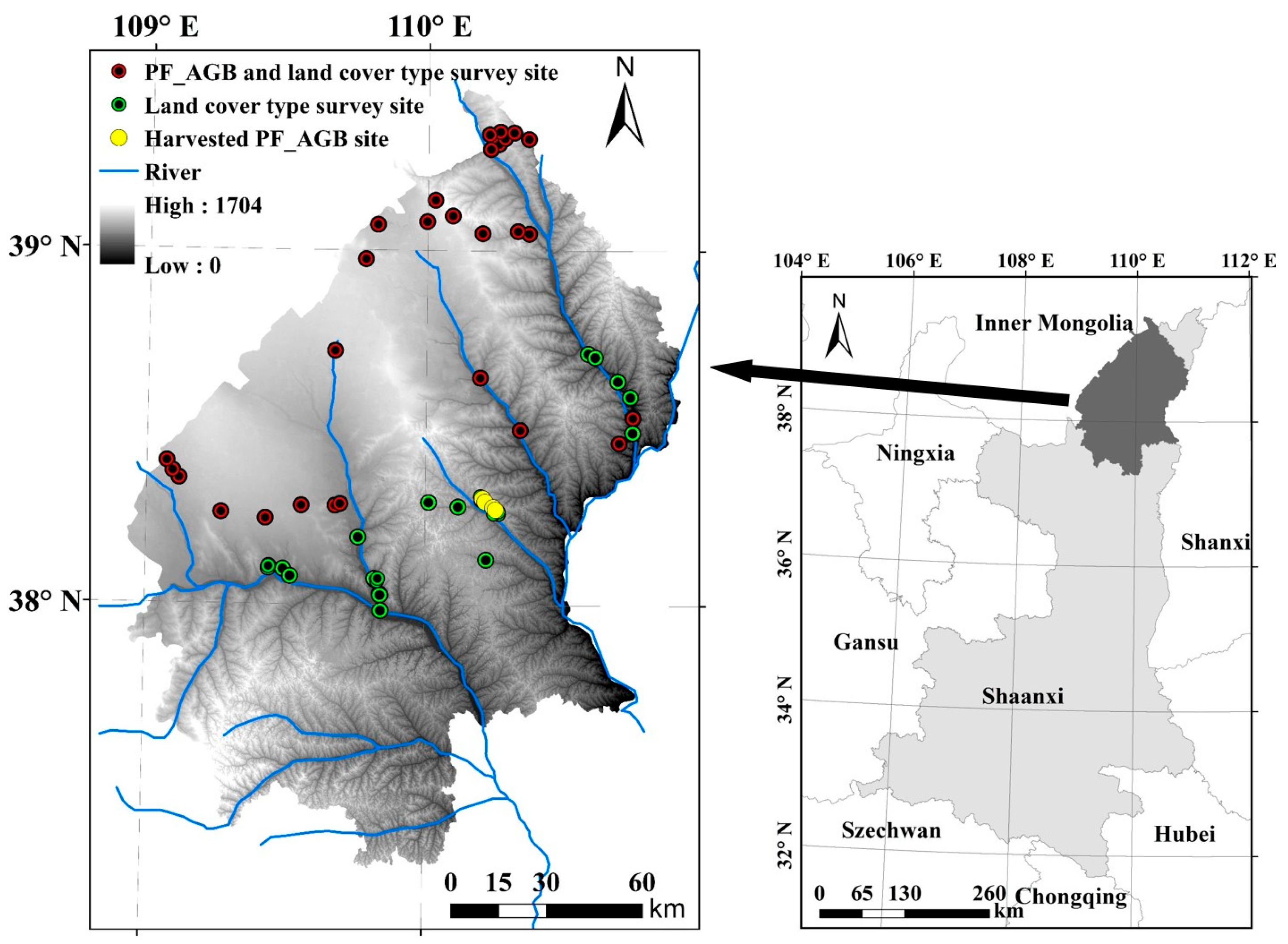
2.1. Study Area
2.2. Data
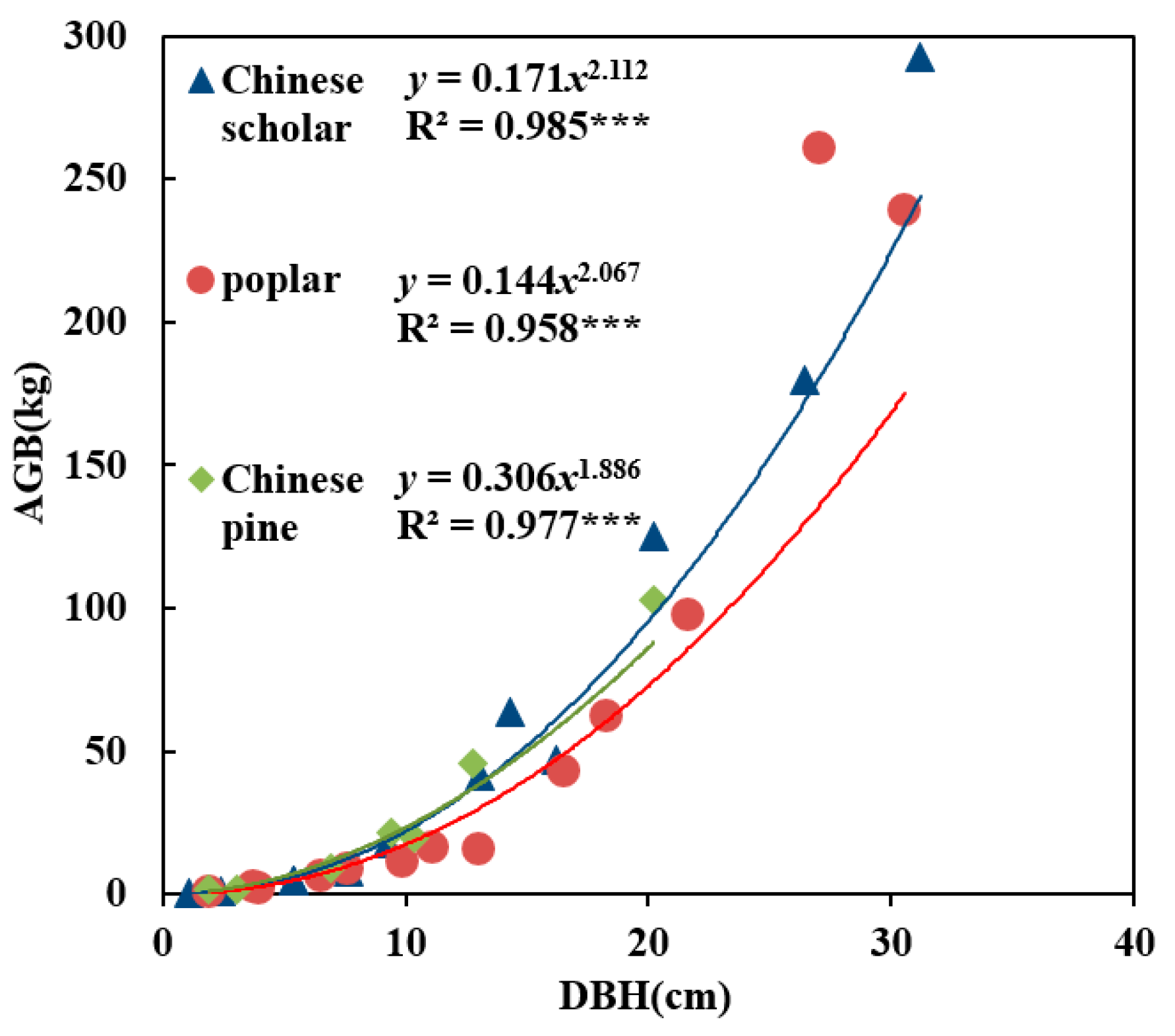
2.2.1. Field Data
2.2.2. Remote Sensing Data
2.2.3. Meteorological Data
2.3. Pixel-Level Stand Age Estimation
2.4. Models for Forest Aboveground Biomass Estimation
3. Results
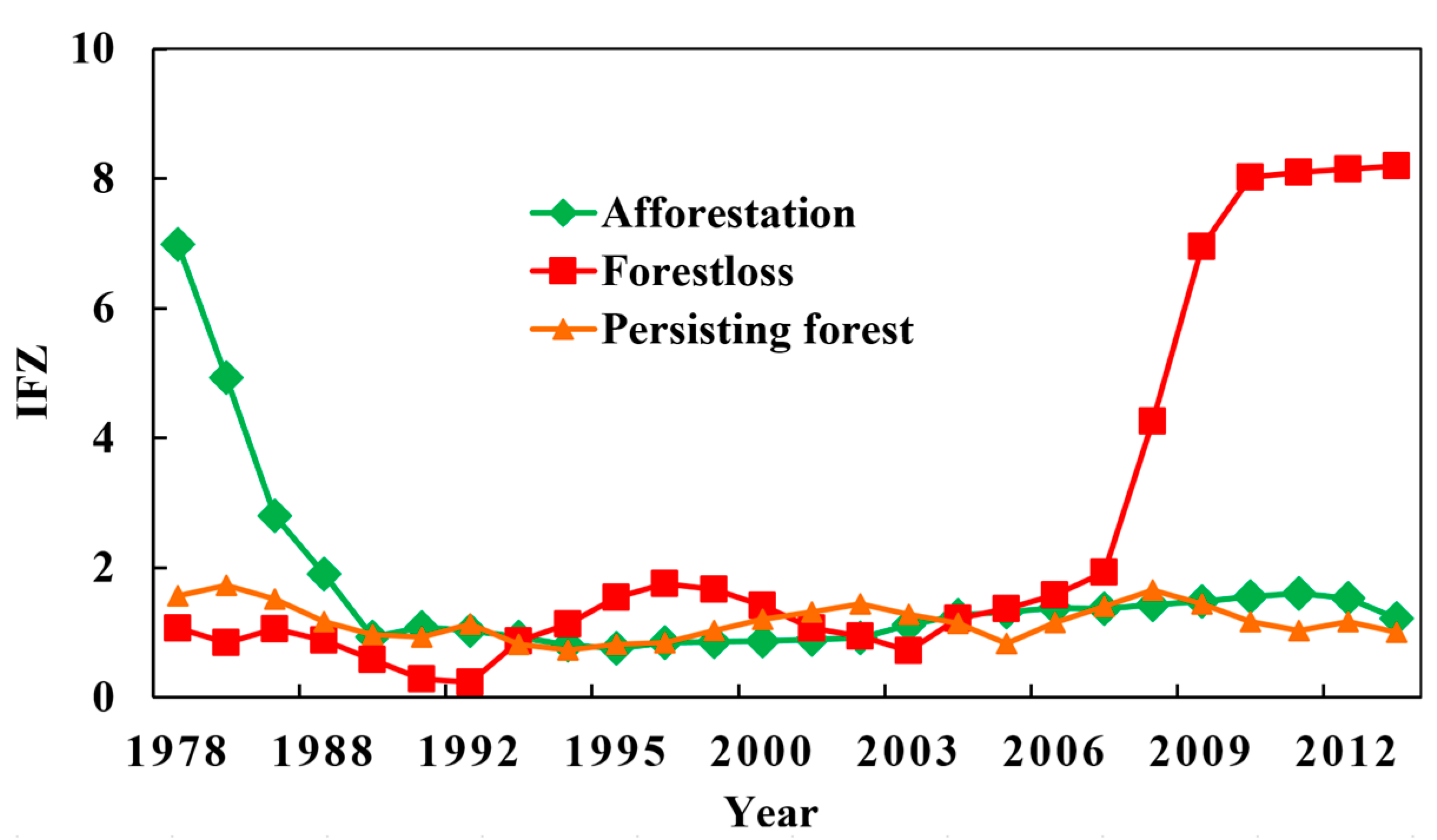
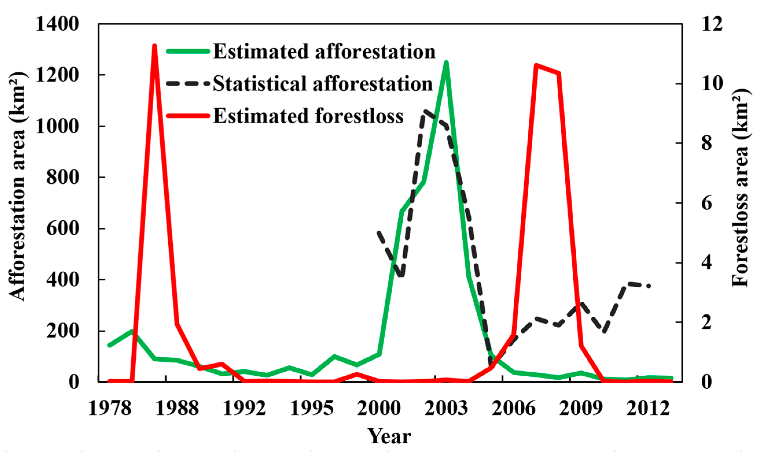
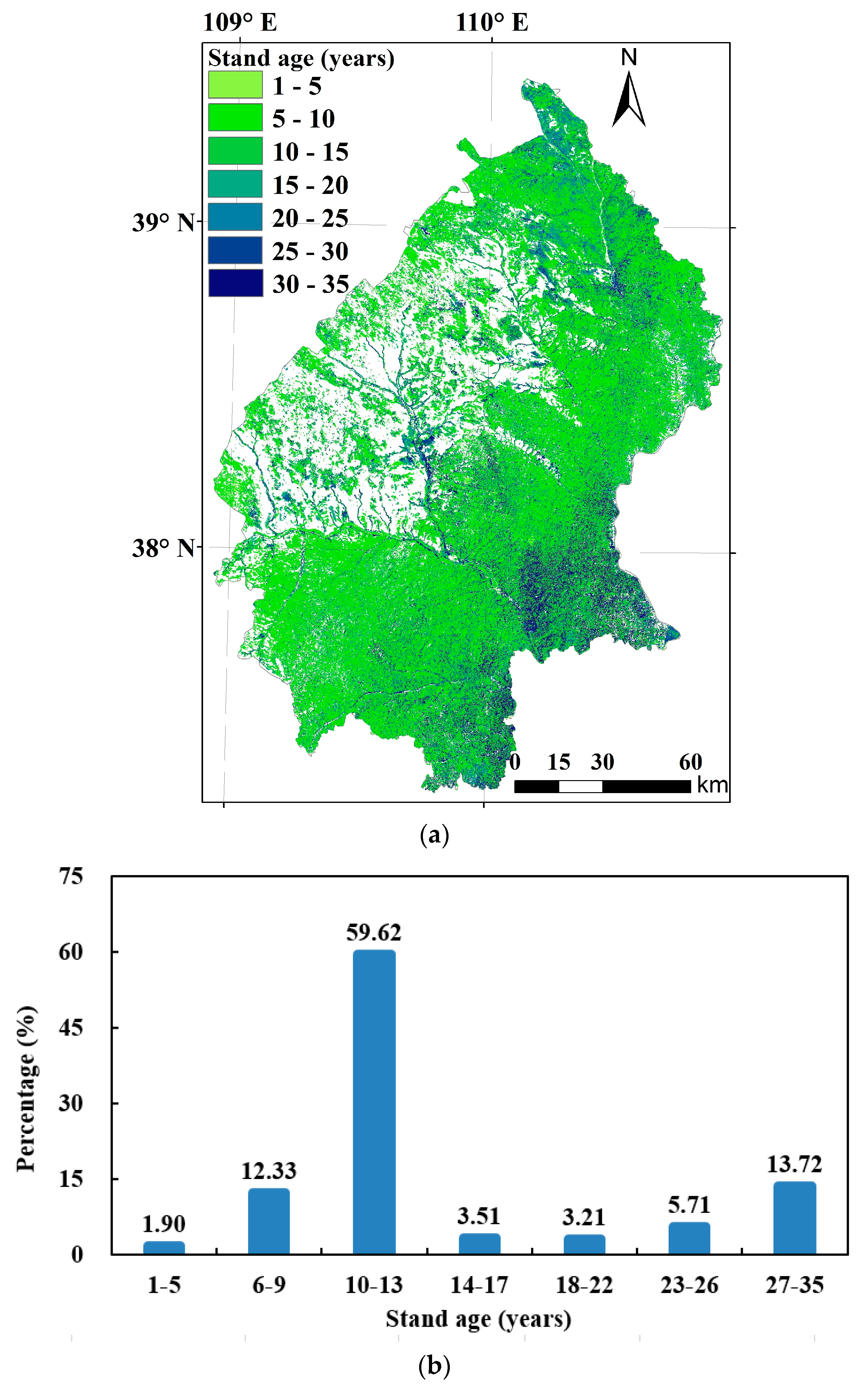
3.1. Afforestation Area and Stand Age
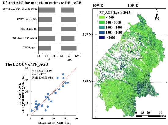
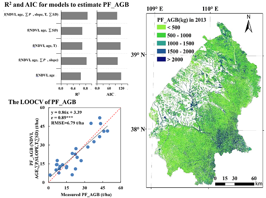
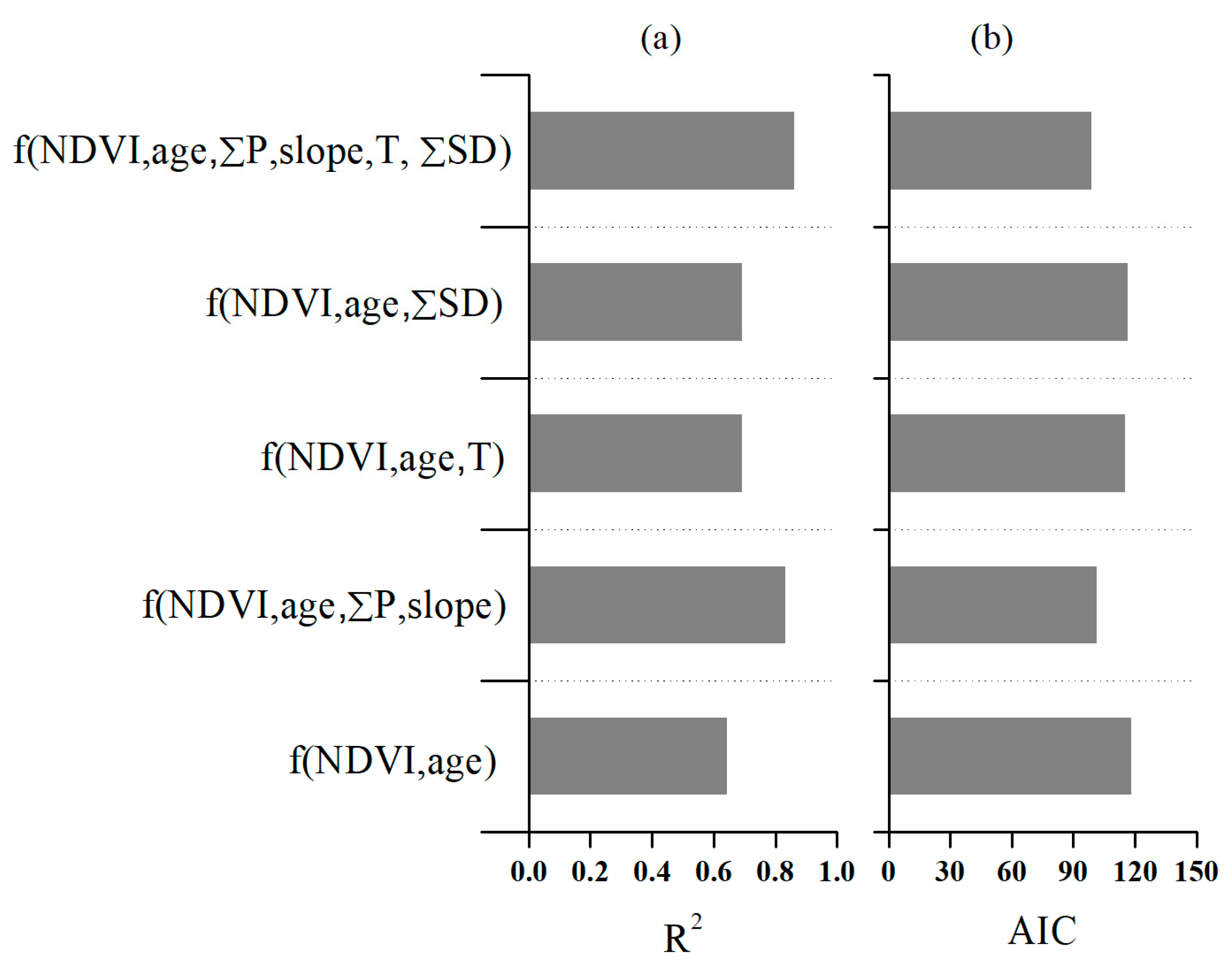
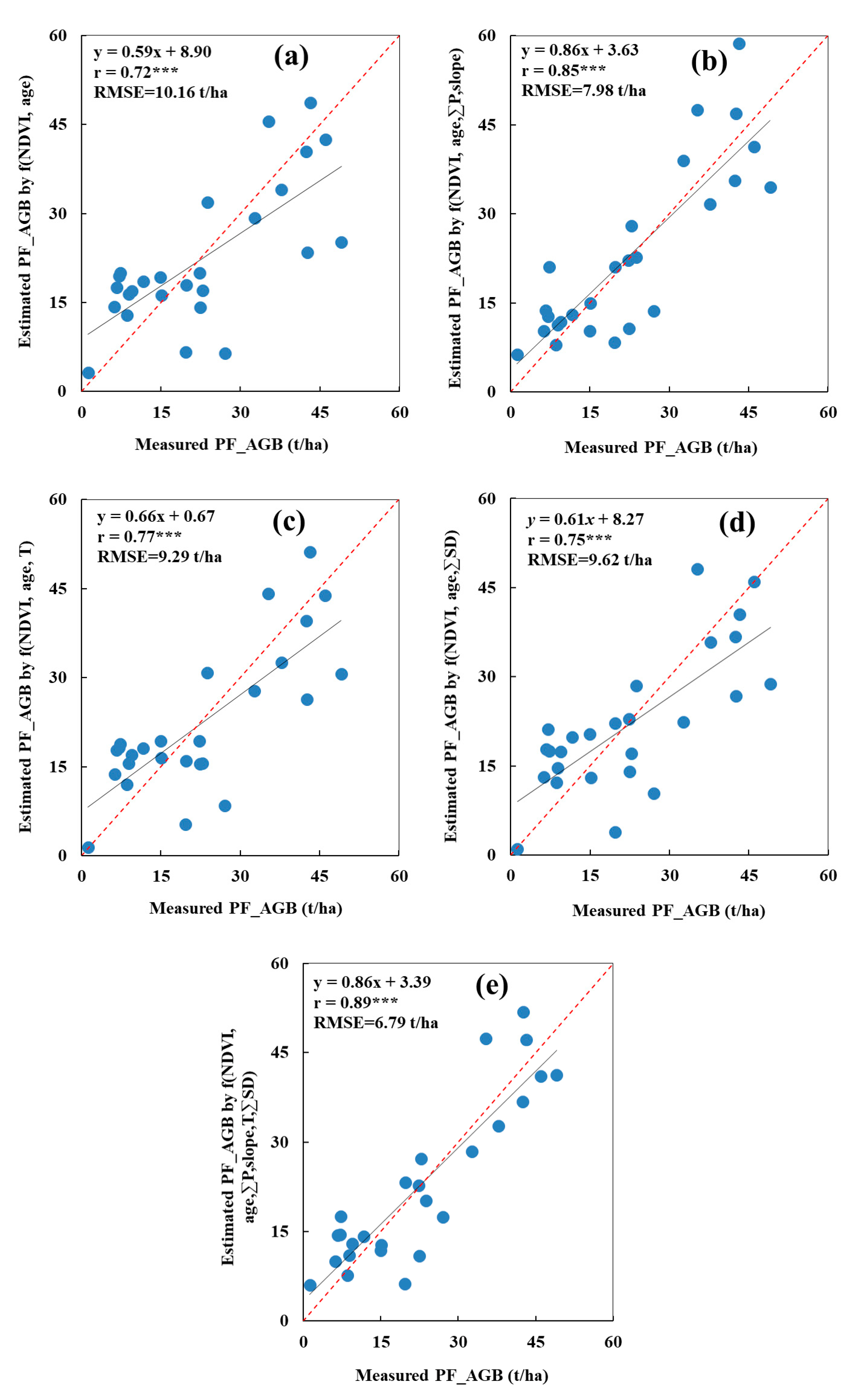
3.2. Planted Forest Aboveground Biomass Estimation and Validation
4. Discussions
4.1. The Relationships of Vegetation Indices and Stand Age with Forest Biomass
4.2. The Influence of Environmental Variables on Tree Growth, Biomass, and Model Performance
5. Conclusions
Author Contributions
Funding
Acknowledgments
Conflicts of Interest
References
- Fang, J.; Chen, A. Dynamic forest biomass carbon pools in China and their significance. Acta Bot. Sin. 2001, 43, 967–973. [Google Scholar] [CrossRef]
- Dixon, R.K.; Solomon, A.M.; Brown, S.; Houghton, R.A.; Trexier, M.C.; Wisniewski, J. Carbon pools and flux of global forest ecosystems. Science 1994, 263, 185–190. [Google Scholar] [CrossRef] [PubMed]
- Fang, J.; Chen, A.; Peng, C.; Zhao, S.; Ci, L. Changes in forest biomass carbon storage in china between 1949 and 1998. Science 2001, 292, 2320–2322. [Google Scholar] [CrossRef] [PubMed]
- Sanna, K.; Anssi, K.; Jari, L.; Pasi, R.; Harri, K.; Mikko, K.; Eetu, P.; Kati, A.; Raisa, M. Change detection of tree biomass with terrestrial laser scanning and quantitative structure modelling. Remote Sens. 2014, 6, 3906–3922. [Google Scholar] [CrossRef]
- Botelho, A.; Lourenço-Gomes, L.; Pinto, L.; Sousa, S.; Valente, M. Using stated preference methods to assess environmental impacts of forest biomass power plants in Portugal. Environ. Dev. Sustain. 2016, 18, 1323–1337. [Google Scholar] [CrossRef] [Green Version]
- Timothy, D.; Onisimo, M.; Cletah, S.; Adelabu, S.; Tsitsi, B. Remote sensing of aboveground forest biomass: A review. Trop. Ecol. 2016, 57, 125–132. [Google Scholar]
- Liu, L.; Peng, D.; Wang, Z.; Hu, Y. Improving artificial forest biomass estimates using afforestation age information from time series landsat stacks. Environ. Monit. Assess. 2014, 186, 7293–7306. [Google Scholar] [CrossRef] [PubMed]
- Zheng, X.; Zhu, J. A methodological approach for spatial downscaling of TRMM precipitation data in north China. Int. J. Remote Sens. 2015, 36, 144–169. [Google Scholar] [CrossRef]
- Wang, H.; Hao, Z. A simulation study on the eco-environmental effects of 3N Shelterbelt in north China. Glob. Planet. Chang. 2003, 37, 231–246. [Google Scholar] [CrossRef]
- Duan, H.; Yan, C.; Tsunekawa, A.; Song, X.; Li, S.; Xie, J. Assessing vegetation dynamics in the Three-North Shelter Forest region of China using AVHRR NDVI data. Environ. Earth Sci. 2011, 64, 1011–1020. [Google Scholar] [CrossRef]
- Li, S.; Zhai, H. The comparison study on forestry ecological projects in the world. Acta Ecol. Sin. 2002, 22, 1976–1982. [Google Scholar] [CrossRef]
- Zhu, J.; Li, F.; Xu, M.; Kang, H.; Wu, X. The role of ectomycorrhizal fungi in alleviating pine decline in semiarid sandy soil of northern China: An experimental approach. Ann. For. Sci. 2008, 65, 304. [Google Scholar] [CrossRef]
- Yu, L.; Wang, J.; Gong, P. Improving 30 meter global land cover map FROM-GLC with time series MODIS and auxiliary datasets: A segmentation based approach. Int. J. Remote Sens. 2013, 34, 5851–5867. [Google Scholar] [CrossRef]
- Zhang, B.; Tong, Q.; Zheng, L.; Wang, J.; Wang, X. Study on the land cover change in the Loess Plateau of China. J. Arid Land Stud. 1998, 8, 13–18. [Google Scholar]
- Yan, Q.L.; Zhu, J.J.; Hu, Z.B.; Sun, O.J. Environmental impacts of the shelter forests in Horqin Sandy land, northeast China. J. Environ. Qual. 2011, 40, 815–824. [Google Scholar] [CrossRef] [PubMed]
- Ji, C.; Li, X.; Jia, Y.; Wang, L. Dynamic assessment of soil water erosion in the Three-North Shelter Forest Region of China from 1980 to 2015. Eurasian Soil Sci. 2018, 51, 1533–1546. [Google Scholar] [CrossRef]
- Segura, M.; Kanninen, M. Allometric models for tree volume and total aboveground biomass in a tropical humid forest in Costa Rica. Biotropica 2005, 37, 2–8. [Google Scholar] [CrossRef]
- Somogyi, Z.; Cienciala, E.; Mäkipää, R.; Muukkonen, P.; Lehtonen, A.; Weiss, P. Indirect methods of large-scale forest biomass estimation. Eur. J. For. Res. 2007, 126, 197–207. [Google Scholar] [CrossRef]
- Brown, S. Estimating Biomass and Biomass Change of Tropical Forests: A Primer; FAO Forestry Paper 134; Food and Agriculture Organization: Rome, Italy, 1997. [Google Scholar]
- Zolkos, S.; Goetz, S.; Dubayah, R. A meta-analysis of terrestrial aboveground biomass estimation using LiDAR remote sensing. Remote Sens. Environ. 2013, 128, 289–298. [Google Scholar] [CrossRef]
- Gibbs, H.K.; Brown, S.; Niles, J.O.; Foley, J.A. Monitoring and estimating tropical forest carbon stocks: Making REDD a reality. Environ. Res. Lett. 2007, 2, 045023. [Google Scholar] [CrossRef]
- Yu, L.; Wang, J.; Li, X.; Li, C.; Zhao, Y.; Gong, P. A multi-resolution global land cover dataset through multisource data aggregation. Sci. China Earth Sci. 2014, 57, 2317–2329. [Google Scholar] [CrossRef]
- Li, Z.; Li, X.; Wang, Y.; Ma, A.; Wang, J. Land-use change analysis in Yulin prefecture, northwestern China using remote sensing and GIS. Int. J. Remote Sens. 2004, 25, 5691–5703. [Google Scholar] [CrossRef]
- Jiang, Y.; Wang, W.; Wang, Z.; Hu, G.; Lei, H. The soil erosion in the north of Shaanxi province of the Loess Plateau and its synthesizing harness. Res. Soil Water Conserv. 1999, 6, 174–180. [Google Scholar]
- Wang, C. Biomass allometric equations for 10 co-occurring tree species in Chinese temperate forests. For. Ecol. Manag. 2006, 222, 9–16. [Google Scholar] [CrossRef]
- Niklas, K.J. Plant Allometry: The Scaling of Form and Process; University of Chicago Press: Chicago, IL, USA, 1994. [Google Scholar] [CrossRef]
- Gower, S.T.; Kucharik, C.J.; Norman, J.M. Direct and indirect estimation of leaf area index, fAPAR, and net primary production of terrestrial ecosystems. Remote Sens. Environ. 1999, 70, 29–51. [Google Scholar] [CrossRef]
- Huang, C.; Goward, S.N.; Masek, J.G.; Gao, F.; Vermote, E.F.; Thomas, N.; Schleeweis, K.; Kennedy, R.E.; Zhu, Z.; Eidenshink, J.C.; et al. Development of time series stacks of Landsat images for reconstructing forest disturbance history. Int. J. Digit. Earth 2009, 2, 195–218. [Google Scholar] [CrossRef]
- Liu, L.; Tang, H.; Caccetta, P.; Lehmann, E.A.; Wu, X. Mapping afforestation and deforestation from 1974 to 2012 using Landsat time-series stacks in Yulin District, a key region of the Three-North Shelter region, China. Environ. Monit. Assess. 2013, 185, 9949–9965. [Google Scholar] [CrossRef]
- Vermote, E.F.; Tanré, D.; Deuze, J.L.; Herman, M.; Morcette, J.J. Second simulation of the satellite signal in the solar spectrum, 6s: An overview. IEEE Trans. Geosci. Remote. Sens. 1997, 35, 675–686. [Google Scholar] [CrossRef]
- Peng, D.; Huang, J.; Cai, C.; Deng, R.; Xu, J. Assessing the response of seasonal variation of net primary productivity to climate using remote sensing data and geographic information system techniques in Xinjiang. J. Integr. Plant Biol. 2008, 50, 1580–1588. [Google Scholar] [CrossRef]
- Peng, D.; Wu, C.; Zhang, B.; Huete, A.; Zhang, X.; Sun, R.; Lei, L.; Huang, W.; Liu, L.; Liu, X.; et al. The influences of drought and land-cover conversion on inter-annual variation of NPP in the Three-North Shelterbelt Program zone of China based on MODIS data. PLoS ONE 2016, 11, e0158173. [Google Scholar] [CrossRef]
- Huang, C.; Goward, S.N.; Masek, J.G.; Thomas, N.; Zhu, Z.; Vogelmann, J.E. An automated approach for reconstructing recent forest disturbance history using dense Landsat time series stacks. Remote Sens. Environ. 2010, 114, 183–198. [Google Scholar] [CrossRef]
- Akaike, H. Factor analysis and AIC. Psychometrika 1987, 52, 317–332. [Google Scholar] [CrossRef]
- Bryan, B.; Gao, L.; Ye, Y.; Sun, X.; Connor, J.; Crossman, N.; Stafford-Smith, M.; Wu, J.; He, C.; Yu, D.; et al. China’s response to a national land-system sustainability emergency. Nature 2018, 559, 193–204. [Google Scholar] [CrossRef]
- Lu, F.; Hu, H.; Sun, W.; Zhu, J.; Liu, G.; Zhou, W.; Zhang, Q.; Shi, P.; Liu, X.; Wu, X.; et al. Effects of national ecological restoration projects on carbon sequestration in China from 2001 to 2010. Proc. Natl. Acad. Sci. USA 2018, 115, 4039–4044. [Google Scholar] [CrossRef] [PubMed] [Green Version]
- Shao, J. Linear model selection by cross-validation. J. Am. Stat. Assoc. 1993, 88, 486–494. [Google Scholar] [CrossRef]
- Steininger, M.K. Satellite estimation of tropical secondary forest above-ground biomass: Data from Brazil and Bolivia. Int. J. Remote Sens. 2000, 21, 1139–1157. [Google Scholar] [CrossRef]
- Makela, H.; Pekkarinen, A. Estimation of forest stand volumes by Landsat TM imagery and stand-level field-inventory data. For. Ecol. Manag. 2004, 196, 245–255. [Google Scholar] [CrossRef]
- Madugundu, R.; Nizalapur, V.; Jha, C.S. Estimation of LAI and above-ground biomass in deciduous forests: Western Ghats of Karnataka, India. Int. J. Appl. Earth Obs. 2008, 10, 211–219. [Google Scholar] [CrossRef]
- Du, H.; Cui, R.; Zhou, G.; Shi, Y.; Xu, X.; Fan, W.; Lü, Y. The responses of Moso bamboo (Phyllostachys heterocycla var. pubescens) forest aboveground biomass to Landsat TM spectral reflectance and NDVI. Acta Ecol. Sin. 2010, 30, 257–263. [Google Scholar] [CrossRef]
- Cao, L.; Coops, N.C.; Innes, J.L.; Sheppard, S.R.J.; Fu, L.; Ruan, H.; She, G. Estimation of forest biomass dynamics in subtropical forests using multi-temporal airborne LiDAR data. Remote Sens. Environ. 2016, 178, 158–171. [Google Scholar] [CrossRef]
- Basuki, T.M.; Skidmore, A.K.; Hussin, Y.A.; Duren, I.V. Estimating tropical forest biomass more accurately by integrating ALOS PALSAR and Landsat-7 ETM+ data. Int. J. Remote Sens. 2013, 34, 4871–4888. [Google Scholar] [CrossRef] [Green Version]
- Lu, D.; Chen, Q.; Wang, G.; Moran, E.; Batistella, M.; Zhang, M.; Laurin, G.; Saah, D. Aboveground forest biomass estimation with Landsat and LiDAR data and uncertainty analysis of the estimates. Int. J. For. Res. 2012, 2012, 436537. [Google Scholar] [CrossRef]
- Foody, G.M.; Boyd, D.S.; Cutler, M.E.J. Predictive relations of tropical forest biomass from Landsat TM data and their transferability between regions. Remote Sens. Environ. 2003, 85, 463–474. [Google Scholar] [CrossRef]
- Rouse, J.W., Jr.; Haas, R.H.; Schell, J.A.; Deering, D.W.; Schell, J.A. Monitoring the Vernal Advancement and Retrogradation (Green Wave Effect) of Natural Vegetation. Prog. Rep. RSC 1978-1; NTIS No. E73-106393; Remote Sensing Center, Texas A&M University: College Station, TX, USA, 1973; 93p. [Google Scholar]
- Thenkabail, S.P.; Lyon, G.J.; Huete, A. Hyperspectral Remote Sensing of Vegetation; CRC Press: Boca Raton, FL, USA, 2011. [Google Scholar]
- Huete, A.; Liu, H.; Batchily, K.; Leeuwen, W. A comparison of vegetation indices over a global set of TM images for EOS-MODIS. Remote Sens. Environ. 1997, 59, 440–451. [Google Scholar] [CrossRef]
- Peng, D.; Zhang, H.; Yu, L.; Wu, M.; Wang, F.; Huang, W.; Liu, L.; Sun, R.; Li, C.; Wang, D.; et al. Assessing spectral indices to estimate the fraction of photosynthetically active radiation absorbed by the vegetation canopy. Int. J. Remote Sens. 2018, 39, 8022–8040. [Google Scholar] [CrossRef]
- Lei, J.; Albert, J.P. Performance Evaluation of Spectral Vegetation Indices Using a Statistical Sensitivity Function. Remote Sens. Environ. 2007, 106, 59–65. [Google Scholar] [CrossRef]
- He, L.; Chen, J.M.; Pan, Y.; Birdsey, R.; Kattge, J. Relationships between net primary productivity and forest stand age in U.S. forests. Glob. Biogeochem. Cycles 2012, 26, GB3009. [Google Scholar] [CrossRef]
- Condit, R.; Ashton, P.S.; Baker, P.; Bunyavejchewin, S.; Gunatilleke, S.; Gunatilleke, N.; Hubbell, S.P.; Foster, R.B.; Itoh, A.; LaFrankie, J.; et al. Spatial patterns in the distribution of tropical tree species. Science 2000, 288, 1414–1418. [Google Scholar] [CrossRef]
- Ge, J.; Xie, Z. Geographical and climatic gradients of evergreen versus deciduous broad-leaved tree species in subtropical China: Implications for the definition of the mixed forest. Ecol. Evol. 2017, 7, 3636–3644. [Google Scholar] [CrossRef] [Green Version]
- Dulamsuren, C.; Hauck, M.; Mühlenberg, M. Vegetation at the taiga forest-steppe borderline in the Western Khentey Mountains, northern Mongolia. Ann. Bot. Fenn. 2005, 42, 411–426. [Google Scholar] [CrossRef]
- Lawson, S.S.; Michler, C.H. Afforestation, restoration and regeneration—Not all trees are created equal. J. For. Res. 2014, 25, 3–20. [Google Scholar] [CrossRef]
- Zhukov, A.B.; Savin, E.N.; Korotkov, I.A.; Ogorodnikov, A.B. Forests of the Mongolian People’s Republic (geography and classification). Biol. Resur. Prir. Usloviy MNR 1978, 11, 1–128. (In Russian) [Google Scholar]
- Gerelbaatar, S.; Batsaikhan, G.; Tsogtbaatar, J.; Battulga, P.; Baatarbileg, N.; Gradel, A. Assessment of early survival and growth of planted Scots pine (Pinus sylvestris) seedlings under extreme continental climate conditions of northern Mongolia. J. For. Res. 2019. [Google Scholar] [CrossRef]
- Williams, A.P.; Allen, C.D.; Macalady, A.K. Temperature as a potent driver of regional forest drought stress and tree mortality. Nat. Clim. Chang. 2013, 3, 292–297. [Google Scholar] [CrossRef]
- Gradel, A.; Haensch, C.; Ganbaatar, B.; Batdorj, D.; Ochirragchaa, N.; Gu¨nther, B. Response of white birch (Betula platyphylla Sukaczev) to temperature and precipitation in the mountain forest steppe and taiga of northern Mongolia. Dendrochronologia 2017, 4, 24–33. [Google Scholar] [CrossRef]
- Nemani, R.R.; Keeling, C.D.; Hashimoto, H.; William, M.J.; Stephen, C.P.; Compton, J.T.; Ranga, M.B.; Running, S.W. Climate–driven increases in global terrestrial net primary production from 1982 to 1999. Science 2003, 300, 1560–1563. [Google Scholar] [CrossRef] [PubMed]
- Ollinger, S.V.; Goodale, C.L.; Hayhoe, K.; Jenkins, J.P. Potential effects of climate change and rising CO2 on ecosystem processes in northeastern U.S. forests. Mitig. Adapt. Strateg. Glob. 2008, 13, 467–485. [Google Scholar] [CrossRef]
- Thompson, J.R.; Foster, D.R.; Scheller, R.; Kittredge, D. The influence of land use and climate change on forest biomass and composition in Massachusetts, USA. Ecol. Appl. 2011, 21, 2425–2444. [Google Scholar] [CrossRef] [Green Version]
- Luizao, R.C.C.; Luizao, F.J.; Paiva, R.Q.; Monteiro, T.F.; Sousa, L.S.; Kruijts, B. Variation of carbon and nitrogen cycling processes along a topographic gradient in a central Amazonian forest. Glob. Chang. Biol. 2010, 10, 592–600. [Google Scholar] [CrossRef]
- Larsen, D.R.; Speckman, P.L. Multivariate regression trees for analysis of abundance data. Biometrics 2015, 60, 543–549. [Google Scholar] [CrossRef]
- Dulamsuren, C.; Hauck, M. Spatial and seasonal variation of climate on steppe slopes of the northern Mongolian mountain taiga. Grassl. Sci. 2008, 54, 217–230. [Google Scholar] [CrossRef]
- Xu, Y.; Franklin, S.; Wang, Q.; Shi, Z.; Luo, Y.; Lu, Z.; Zhang, J.; Qiao, X.; Jiang, M. Topographic and biotic factors determine forest biomass spatial distribution in a subtropical mountain moist forest. For. Ecol. Manag. 2015, 357, 95–103. [Google Scholar] [CrossRef]
- Lu, D. The potential and challenge of remote sensing-based biomass estimation. Int. J. Remote Sens. 2006, 27, 1297–1328. [Google Scholar] [CrossRef]
- Lu, D. Aboveground biomass estimation using Landsat TM data in the Brazilian Amazon. Int. J. Remote Sens. 2005, 26, 2509–2525. [Google Scholar] [CrossRef]
- Lu, D.; Mausel, P.; Brondizio, E.; Moran, E. Relationships between forest stand parameters and Landsat TM spectral responses in the Brazilian Amazon Basin. For. Ecol. Manag. 2004, 198, 149–167. [Google Scholar] [CrossRef]
- Sarker, L.R.; Nichol, J.E. Improved forest biomass estimates using alos avnir-2 texture indices. Remote Sens. Environ. 2011, 115, 968–977. [Google Scholar] [CrossRef]
- Gleason, C.J.; Im, J. Forest biomass estimation from airborne LiDAR data using machine learning approaches. Remote Sens. Environ. 2012, 125, 80–91. [Google Scholar] [CrossRef]
- Knapp, N.; Fischer, R.; Huth, A. Linking LiDAR and forest modeling to assess biomass estimation across scales and disturbance states. Remote Sens. Environ. 2018, 205, 199–209. [Google Scholar] [CrossRef]
- Luo, S.; Wang, C.; Xi, X.; Pan, F.; Peng, D.; Zou, J.; Nie, S.; Qin, H. Fusion of airborne LiDAR data and hyperspectral imagery for aboveground and belowground forest biomass estimation. Ecol. Indic. 2017, 73, 378–387. [Google Scholar] [CrossRef]
- Glenn, N.F.; Neuenschwander, A.; Vierling, L.A.; Spaete, L.; Li, A.; Shinneman, D.J.; Pilliod, D.; Arkle, R.; Mcllroy, S. Landsat 8 and ICESat-2: Performance and potential synergies for quantifying dryland ecosystem vegetation cover and biomass. Remote Sens. Environ. 2016, 185, 233–242. [Google Scholar] [CrossRef]


© 2019 by the authors. Licensee MDPI, Basel, Switzerland. This article is an open access article distributed under the terms and conditions of the Creative Commons Attribution (CC BY) license (http://creativecommons.org/licenses/by/4.0/).
Share and Cite
Peng, D.; Zhang, H.; Liu, L.; Huang, W.; Huete, A.R.; Zhang, X.; Wang, F.; Yu, L.; Xie, Q.; Wang, C.; et al. Estimating the Aboveground Biomass for Planted Forests Based on Stand Age and Environmental Variables. Remote Sens. 2019, 11, 2270. https://doi.org/10.3390/rs11192270
Peng D, Zhang H, Liu L, Huang W, Huete AR, Zhang X, Wang F, Yu L, Xie Q, Wang C, et al. Estimating the Aboveground Biomass for Planted Forests Based on Stand Age and Environmental Variables. Remote Sensing. 2019; 11(19):2270. https://doi.org/10.3390/rs11192270
Chicago/Turabian StylePeng, Dailiang, Helin Zhang, Liangyun Liu, Wenjiang Huang, Alfredo R. Huete, Xiaoyang Zhang, Fumin Wang, Le Yu, Qiaoyun Xie, Cheng Wang, and et al. 2019. "Estimating the Aboveground Biomass for Planted Forests Based on Stand Age and Environmental Variables" Remote Sensing 11, no. 19: 2270. https://doi.org/10.3390/rs11192270