Article

Evaluating k-Nearest Neighbor (kNN) Imputation Models for Species-Level Aboveground Forest Biomass Mapping in Northeast China

1
Key Laboratory of Geographical Processes and Ecological Security in Changbai Mountains, Ministry of Education, School of Geographical Sciences, Northeast Normal University, Changchun 130024, China
2
School of Natural Resources, University of Missouri, Columbia, MO 65211, USA
3
U.S. Geological Survey, Denver Federal Center, MS 980, Denver, CO 80225, USA
4
U.S. Geological Survey, 12201 Sunrise Valley Drive, Reston, VA 20192, USA
*
Author to whom correspondence should be addressed.
Remote Sens. 2019, 11(17), 2005; https://doi.org/10.3390/rs11172005
Submission received: 26 July 2019 / Revised: 15 August 2019 / Accepted: 21 August 2019 / Published: 25 August 2019
(This article belongs to the Special Issue Forest Biomass and Carbon Observation with Remote Sensing)

Abstract

:
Quantifying spatially explicit or pixel-level aboveground forest biomass (AFB) across large regions is critical for measuring forest carbon sequestration capacity, assessing forest carbon balance, and revealing changes in the structure and function of forest ecosystems. When AFB is measured at the species level using widely available remote sensing data, regional changes in forest composition can readily be monitored. In this study, wall-to-wall maps of species-level AFB were generated for forests in Northeast China by integrating forest inventory data with Moderate Resolution Imaging Spectroradiometer (MODIS) images and environmental variables through applying the optimal k-nearest neighbor (kNN) imputation model. By comparing the prediction accuracy of 630 kNN models, we found that the models with random forest (RF) as the distance metric showed the highest accuracy. Compared to the use of single-month MODIS data for September, there was no appreciable improvement for the estimation accuracy of species-level AFB by using multi-month MODIS data. When k > 7, the accuracy improvement of the RF-based kNN models using the single MODIS predictors for September was essentially negligible. Therefore, the kNN model using the RF distance metric, single-month (September) MODIS predictors and k = 7 was the optimal model to impute the species-level AFB for entire Northeast China. Our imputation results showed that average AFB of all species over Northeast China was 101.98 Mg/ha around 2000. Among 17 widespread species, larch was most dominant, with the largest AFB (20.88 Mg/ha), followed by white birch (13.84 Mg/ha). Amur corktree and willow had low AFB (0.91 and 0.96 Mg/ha, respectively). Environmental variables (e.g., climate and topography) had strong relationships with species-level AFB. By integrating forest inventory data and remote sensing data with complete spatial coverage using the optimal kNN model, we successfully mapped the AFB distribution of the 17 tree species over Northeast China. We also evaluated the accuracy of AFB at different spatial scales. The AFB estimation accuracy significantly improved from stand level up to the ecotype level, indicating that the AFB maps generated from this study are more suitable to apply to forest ecosystem models (e.g., LINKAGES) which require species-level attributes at the ecotype scale.

Graphical Abstract

1. Introduction

Spatially explicit or pixel-level aboveground forest biomass (AFB) information is increasingly needed for estimating forest carbon stocks at regional scales [1,2,3]. Such information is often used in ecological models to predict forest carbon dynamics and the change of forest structure and composition due to succession, disturbances (e.g., fire, pests, and harvest), and climate change [4,5]. Whereas AFB estimation from most previous studies lumped all tree species [2,3,6], species-level AFB provides additional information that is important to understanding forest dynamics and therefore is valuable to forest managers and policy makers [1,7].
Remote sensing data are ideally suited to derive pixel-level aboveground forest biomass across large areas [6,8]. Multispectral remote sensing images have long been an important means to obtain forest cover maps [7,9]. However, remote sensing data alone cannot directly derive the forest attributes necessary for quantifying species-level aboveground forest biomass. In contrast, forest inventory data contain detailed species-level information, but only at limited sample plots, and therefore lack complete spatial coverage. There are numerous methods developed to integrate forest inventory with remote sensing data to generate species-level maps over large spatial extent [10,11].
The k-nearest neighbor (kNN) imputation is one of the most widely used methods to integrate forest attributes and remote sensing data [12]. Due to its ability to estimate more than one forest attribute simultaneously [13], kNN has been increasingly used to predict forest attributes (e.g., stem volume, basal area and aboveground biomass) across large regions [7,14]. For an unsampled target pixel, the kNN method predicts its response variables (forest attributes) firstly by computing the distance metric between the reference samples (neighbors) and the target pixel, and then assigning the mean value of the k nearest neighbors’ response variable to the target pixel [15]. Predictor variables that are common to both the target and reference samples are used to define the feature space, based on which the distance metric is computed [12]. Both the type of distance metric and choice of k value are critical factors influencing the estimation accuracy in kNN imputation [11].
Different combinations of distance metrics and k values have been used in kNN analysis to predict forest attributes [16,17]. In addition to the simple distance metrics (e.g., Euclidean or Mahalanobis) that do not rely on response variables, other distance metrics (RF: random forest, GNN: gradient nearest neighbor, MSN: most similar neighbor and msnPP: most similar neighbor computed using projection pursuit) that closely rely on the response variables have been developed [10,18,19]. Especially the random forest (RF) algorithm, which was incorporated into kNN as a distance metric, has been revealed to be an effective way to impute complex forest attributes [6,20]. The optimal k value (number of the nearest neighbors) used to calculate the forest attributes of the target pixel is not well defined, and unsuitable selection of k value will lead to large errors [15]. Previous studies applying kNN analysis seldom focused on species composition, but only to the structural characteristics of general forest types [21]. Additionally, comparisons of alternative kNN methods with different distance metrics and k values specifically for mapping species composition are rarely reported.
Most recently, based on the combinations of six distance metrics (RF, GNN, MSN, Euclidean, Mahalanobis and msnPP), 15 k values (1–15) and single- vs. multi-month (MODIS) imagery, Zhang et al. [22] compared the prediction accuracy of the 630 kNN models in mapping species-level biomass in Chinese boreal forests. Their results showed good accuracy and the kNN model based on an RF distance metric, k = 6 and single-month MODIS imagery for June was the optimal model for imputing species-level biomass in Chinese boreal forests. However, their study was conducted at a limited spatial extent of Chinese boreal forests with relatively simple species composition. Whether their findings are applicable to larger extents spanning over multiple ecoregions with complex species composition has not been tested. Meanwhile, tree species-level information for multiple ecoregions is increasingly needed for regional-scale assessments.
Our primary objectives were to: (i) extend the 630 kNN models to all of Northeast China, then by evaluating the performance of different models to develop an optimal kNN imputation model to map wall-to-wall, species-level, aboveground forest biomass; (ii) assess the prediction accuracy from the stand to the ecotype level; (iii) analyze the spatial patterns of species-level aboveground forest biomass across different ecoregions in Northeast China; and (iv) investigate the relationship between environmental variables (e.g., climate, topography, soil) and species-level aboveground forest biomass.

2. Materials and Methods
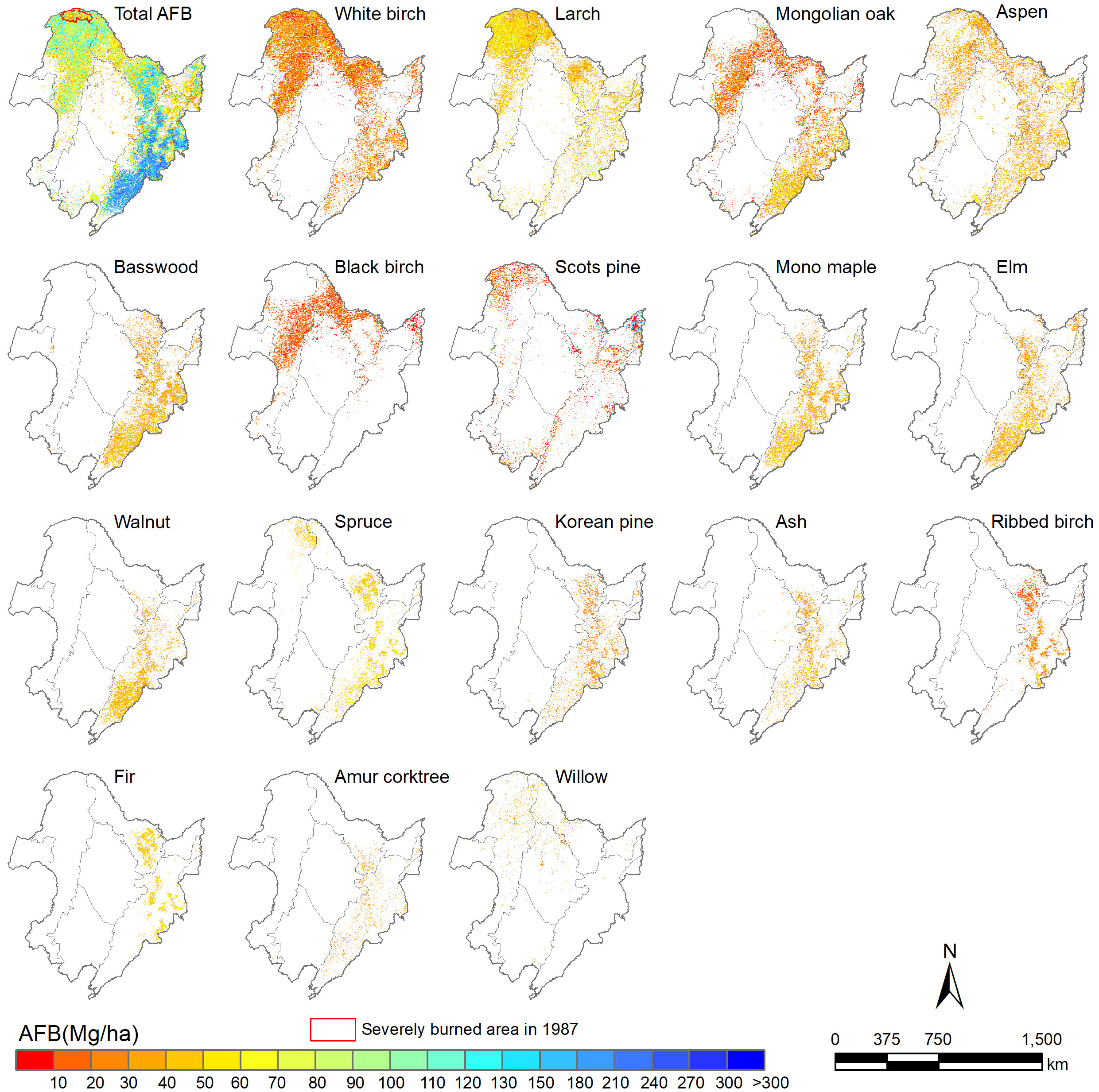
2.1. Study Area

Northeast China (38°42′–53°35′N, 115°32′–135°09′E) includes China’s largest natural forest area, storing nearly half of the total forest biomass in China [23]. The region includes Heilongjiang, Jilin, and Liaoning provinces, and the eastern part of the Inner Mongolia Autonomous Region, covering over 1.24 million km2. According to natural conditions (e.g., temperature, humidity, topography, elevation), Northeast China can be divided into seven major ecoregions [24]: Greater Khingan Mountains (GKM), Lesser Khingan Mountains (LKM), Changbai Mountains (CM), Sanjiang Plain (SJP), Songnen Plain (SNP), Liaohe Plain (LHP) and Hulun Buir Plateau (HBP) (Figure 1). Of these ecoregions, forests are mainly distributed over GKM, LKM and CM. The dominant tree species include three species of larch (Larix gmelinii (Rupr.) Kuzen, Larix olgensis Henry and Larix principis-rupprechtii Mayr), three species of aspen (Populus davidiana Dode, Populus suaveolens Fischer and Populus ussuriensis Kom.), two species of spruce (Picea koraiensis Nakai and Picea jezoensis Carr. var. microsperma (Lindl.) Cheng et L. K. Fu), white birch (Betula platyphylla Suk.), Mongolian oak (Quercus mongolica Fisch. ex Ledeb.), Asian black birch (Betula davurica Pall., hereafter black birch), ribbed birch (Betula costata Trautv.), Mongolian Scots pine (Pinus sylvestris var. mongolica Litv., hereafter Scots pine), basswood (Tilia amurensis Rupr.), mono maple (Acer mono Maxim.), elm (Ulmus pumila L.), Manchurian walnut (Juglans mandshurica Maxim., hereafter walnut), Korean pine (Pinus koraiensis Sieb.et Zucc.), Manchurian ash (Fraxinus mandschurica Rupr., hereafter ash), fir (Abies nephrolepis (Trautv.) Maxim.), Amur corktree (Phellodendron amurense Rupr.), and willow (Chosenia arbutifolia (Pall.) A. Skv.).

2.2. Forest Inventory Data

We obtained data for 25,000 forest stand polygons (average stand size: 20.6 ha) in Northeast China surveyed in the early 2000s from the National Forestry and Grassland Data Center (http://www.cfsdc.org/). The geometric center sites of forest stand polygons are shown in Figure 1. They were mainly distributed in three areas that are representative of forests in Northeast China, the Greater Khingan Mountains, the Lesser Khingan Mountains and the Changbai Mountains [23]. The forest inventory data spanned a variety of forest types (e.g., cold-temperate conifer mixed forests, temperate conifer forests, broadleaf mixed forests, and warm-temperate deciduous broadleaf mixed forests) with different age classes, and include all major tree species in Northeast China. Therefore, the collected forest inventory data in this study effectively represent the species composition and structure of Northeast China. Each forest stand polygon is a contiguous area ranging from a few to tens of hectares that contains a relatively homogeneous tree community and is normally managed as a single unit [25]. The statistics of each forest stand polygon mainly include mean diameter at breast height, stand height, stand age, stand volume, and volume proportion by species. Based on the species-specific biomass-volume relationships [26], we transformed the species-level volume of each forest stand polygon into species-level AFB. In the kNN imputation models, we selected the AFB for the 17 dominant tree species of each stand polygon as the response variables. Additionally, we derived aboveground forest biomass measurements for 143 sample plots spread across the areas where inventory data were sparse (Figure 1) from literatures [27,28]. These added plots were used to validate our imputed total AFB for areas where forest inventory data were not available.

2.3. MODIS Data

MODIS data have wide, complete spatial coverage and a relatively high temporal resolution [7]. We developed mathematical relationships between the rich spectral information in MODIS and species-level AFB from field data [23]. We then applied the kNN imputation method to integrate spatially continuous MODIS data and forest inventory data to derive wall-to-wall species-level AFB over the entirety of Northeast China. Since most of the forest stand polygons were obtained around 2000, the MODIS data (MOD09Q1: b1–b2, 250 m and MOD09A1: b3–b7, 500 m) in 2000 were selected as basic data to derive predictor variables for further AFB mapping. MOD09A1 data were resampled to 250 m using nearest neighbor interpolation to fit the spatial resolution of MOD09Q1 data. To investigate the influences of multi-temporal MODIS data on biomass prediction accuracy, we obtained monthly MOD09Q1 and MOD09A1 data. We extracted the monthly reflectance value of MOD09Q1 and MOD09A1 data by the Maximum Value Composite (MVC) method and average method, respectively. The difference of monthly reflectance extracted by the MVC method was small and the discrimination was not enough to reflect the rich temporal information of monthly MODIS data. The reflectance value of each month extracted by the average method was significantly different, and thus, we selected the monthly average reflectance value (May–October) of MOD09Q1 and MOD09A1 data as predictor variables. Because Northeast China was largely covered by snow or frost during January–April and November–December [23], spectral bands of these two periods were not applied to the kNN models. Several spectral indices (May–October) correlated with vegetation characteristics were also used as predictor variables, which were computed by using the monthly spectral bands (Table 1). Additionally, the 2000 MODIS Vegetation Continuous Fields (VCF) product MOD44B (250 m) was used to extract the forest areas, and pixels with tree cover greater than 10% are defined as forest areas [29]. The 2000 MODIS land cover product MCD12Q1 (500 m) was also resampled to 250 m using nearest neighbor interpolation and used to distinguish different forest types.

2.4. Environmental Data

To reduce uncertainties due to environmental heterogeneity, environmental data related to species-level AFB were selected as auxiliary predictors (Table 1). Topographic data (e.g., slope and cosine of aspect) were derived from a 90 m digital elevation model (DEM) provided by the Shuttle Radar Topography Mission (SRTM) (http://srtm.csi.cgiar.org/) by using ArcGIS 10.3 software. As primary climatic variables, monthly mean temperature and cumulative precipitation data (250 m; 1982-2015) were interpolated from the 103 meteorology stations in Northeast China (https://data.cma.cn/) by using ANUSPLIN 4.3 software, which applied a thin-plate spline function, with the resampled SRTM DEM (250 m) as the covariate [41]. The SRTM DEM was resampled from 90 m to 250 m using bilinear interpolation.
Monthly potential evapotranspiration and radiation data from 1982 to 2015 with a spatial resolution of 0.1° × 0.1° were derived from the China Meteorological Forcing Dataset (http://westdc.westgis.ac.cn). Soil data (1 km resolution) were derived from the Harmonized World Soil Data Base Version 1.2 [42]. In order to preserve the original information of MOD09Q1 data as much as possible, we resampled evapotranspiration data, radiation data, and soil data to the same resolution (250 m) as MODO9Q1 data using nearest neighbor interpolation, and resampled the topographic data (DEM, slope, cosine of aspect) to 250 m resolution using bilinear interpolation.

2.5. Optimizing kNN Models and Species-Level Biomass Imputation

Detailed introduction of the kNN method and its parameters was described in McRoberts et al. [12]. The application of the kNN method entails identifying the k nearest reference samples in the feature space defined by predictor variables for each target unit. Values of each response variable within these k nearest samples are then averaged and assigned to the target unit. Formally, the nearest neighbors prediction, y ˜ i , for the i-th target element is calculated as follows [12]:
Y ˜ i = j = 1 k w i j y i j
where { y i j ;   j = 1 , 2 , , k } is the set of response variable observations for the k reference elements that are nearest to the i-th target element in feature space given a specific distance metric, and w i j is the weight assigned to the j-th nearest neighbor with j = 1 k w i j = 1 . The w i j is defined as follows:
w i j = 1 / ( 1 + d i j ) j = 1 k [ 1 / ( 1 + d i j ) ]
where d i j is the distance in feature space between the j-th nearest neighbor and the i-th target calculated using a given distance metric.
In the process of optimizing kNN models, forest stand polygon was used as the unit of observation. Predictor variables of each stand polygon were calculated as the mean value of the raster pixels with >50% stand cover. The 25,000 stand polygons containing both response variables and predictor variables were split into training and test sets using the 7:3 split ratio. Before building models, redundant predictors were removed using forward stepwise canonical correspondence analysis (CCA) to select significant variables (P < 0.01) [10]. Then, based on six popular distance metrics (RF, GNN, MSN, Euclidean, Mahalanobis, and msnPP), 15 k values (1–15) and seven sets of selected predictor variables, we built 630 kNN models [22]. The process of optimizing the kNN models was executed through kNN prediction analysis based on the training-test sets using yaImpute package in R [43]. For each kNN model, we calculated the multivariate goodness of fit criterion T and the generalized root mean squared distance (GRMSD) as optimization criteria. T is used to measure the quality of multivariate fitting, and larger T values mean better model performance [12]. GRMSD is used to measure the degree of similarity of the structures between the predictive and observed values, and larger GRMSD values mean worse model performance [43]. The multivariate goodness of fit criterion T [12] is defined as:
T = y = 1 Y w y T y 2
where y represents one of the 17 tree species’ AFB, Y is the number of the response variables, w y is the weight of the yth species’ AFB, which is the percent AFB of the yth species against the total AFB based on the observed value. T y 2 is the fractional amount of variance in response variable y explained by the kNN prediction. GRMSD in this study represented the generalized root mean square distance between observed and predictive values in an orthogonal multivariate space defined by AFB values of the 17 species. The optimization exercise was replicated 30 times, yielding the mean values of T and GRMSD. Then, we generated the curves of T vs. k and GRMSD vs. k based on the combinations of different distance metrics and MODIS predictors. For a given combination of distance metric and MODIS predictors, when the T value reached 0.95 of the maximal T value on the curve, the corresponding k value was considered to be optimal [16]. This selected optimal k value was further inspected using GRMSD curves (the k value when GRMSD approximately equalled 1.05 of the minimum GRMSD value on the curve).
After the optimal distance metric, MODIS predictor variables and k value were selected, we applied the optimal kNN model to impute species-level AFB for all the forest pixels with a tree cover >10%. All the processes were implemented in the R software supported by “yaImpute” package (Figure 2).

2.6. Accuracy Assessment

Accuracy assessment of the estimated AFB over Northeast China was performed at the stand and the ecotype level. Ecotype was defined as the unique combination of each landform with forest type in different ecoregions. The seven main ecoregions of Northeast China represented different temperature and moisture conditions. Nine landforms (1: Ridge, 2: Upper slope, 3: Sunny slope, 4: Semi-sunny slope, 5: Semi-shady slope, 6: Shady slope, 7: Flat slope, 8: Lower slope, 9: Bottomland) were classified from DEM using Topographic Position Index [44]. Five forest types (1: evergreen coniferous, 2: evergreen broad-leaved, 3: deciduous coniferous, 4: deciduous broad-leaved, 5: mixed forest) were retrieved from the MCD12Q1 product. For each of the seven ecoregions, 45 ecotypes were generated by combing the nine landforms and five forest types. A total of 315 ecotypes was produced throughout Northeast China.
The estimated AFB of the 30% test dataset at the stand level was calculated by averaging the AFB values of all pixels with over 50% of their area located in each forest stand. Then both the observed and estimated species-level AFB of the test dataset were averaged to the ecotype level. At stand and ecotype levels, we calculated the Pearson correlation (R2), root mean square error (RMSE: Mg/ha), empirical cumulative distribution functions (ECDFs) and the Kolmogorov–Smirnov (KS) statistic [45] between the estimated and observed species-level AFB. R2 and RMSE provide the overall assessment of the estimation accuracy. The ECDFs and KS statistic can quantify the discrepancy in the distributions of the estimated and observed species-level AFB. KS statistic is defined as the maximum distance between observed and estimated ECDFs, without assuming the distribution of the data and independent of the scale changes [46]. We also calculated the R2, RMSE, ECDFs, and KS statistic between the observed and estimated total AFB for the collected 143 sample plots.

3. Results

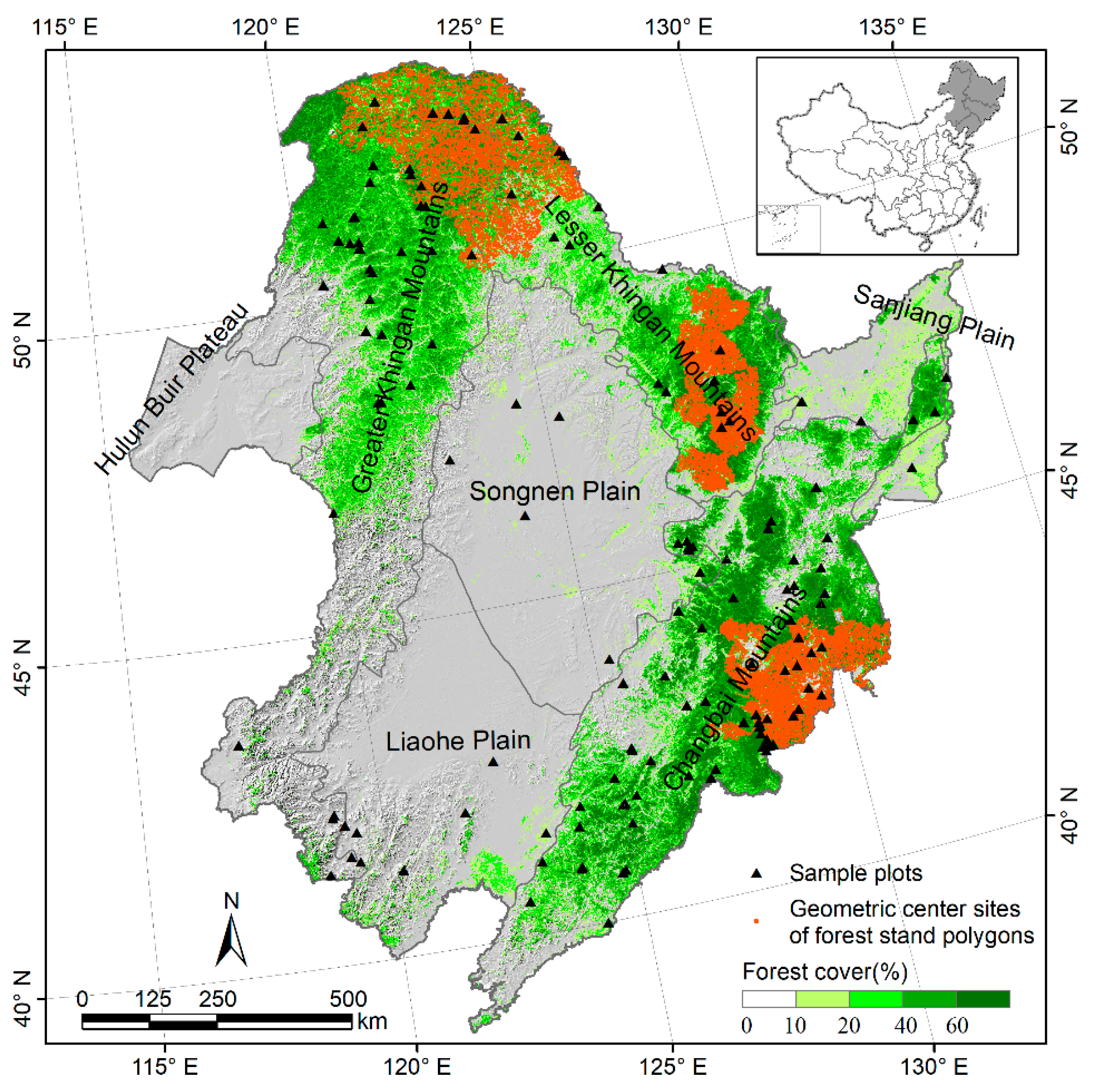
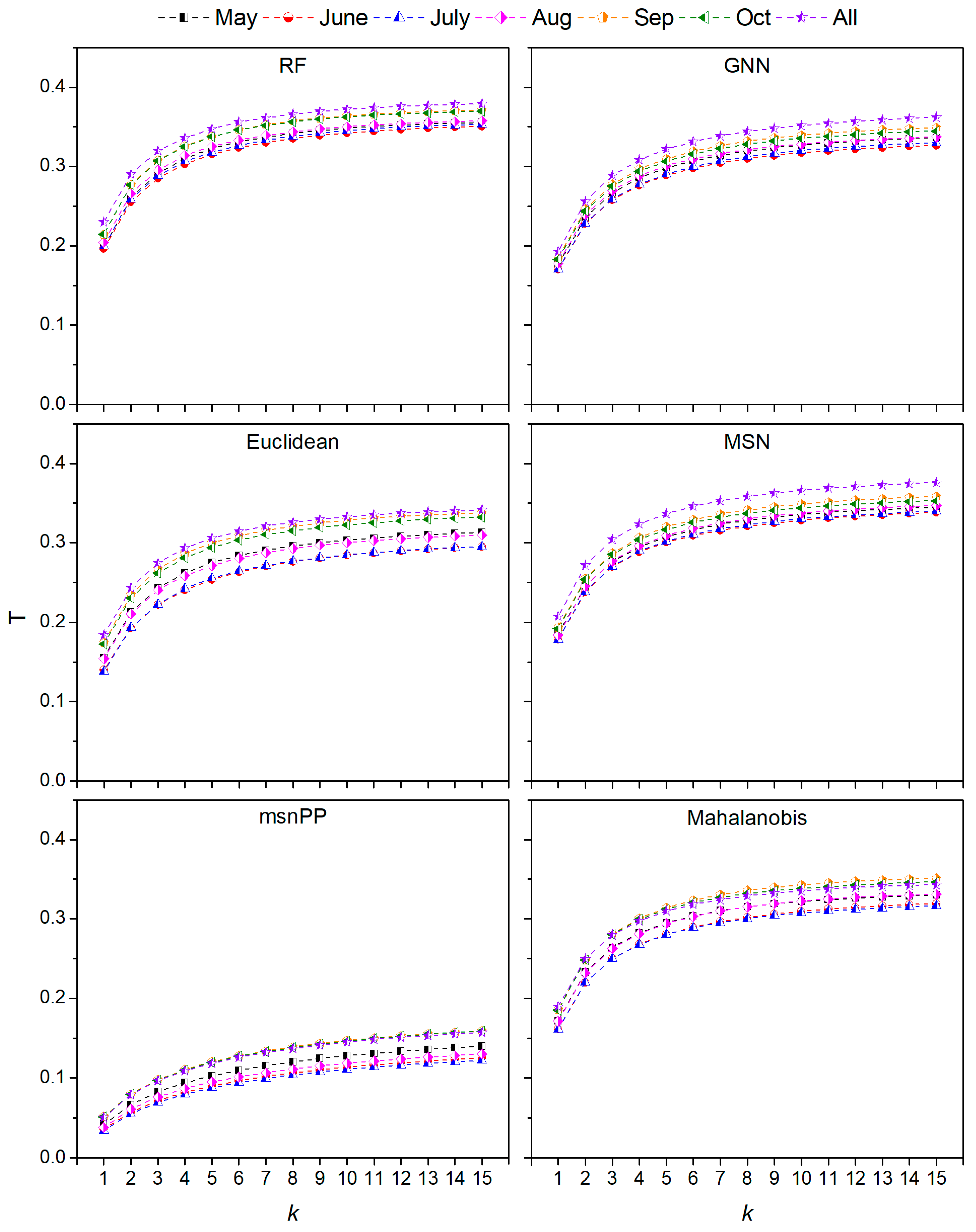
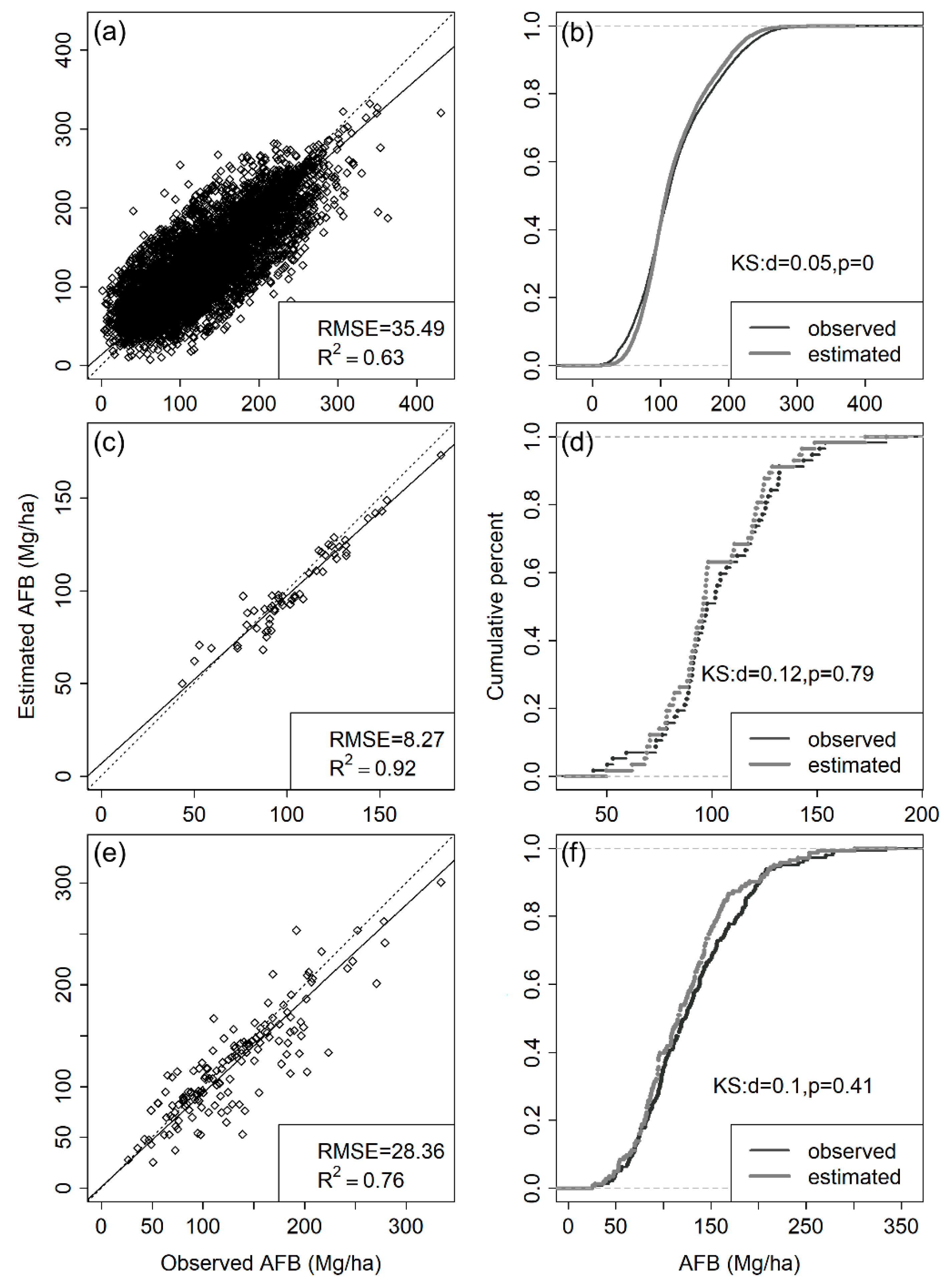
3.1. Performance of Different kNN Models

RF-based kNN models showed the best performance with largest T values and smallest GRMSD values for most of the combinations of k value and MODIS predictor variables, followed closely by MSN- and GNN-based kNN models. The msnPP-based kNN models obviously showed the worst performance with smallest T values and largest GRMSD values (Figure 3 and Figure 4). Compared with single-month predictor variables (September), use of multi-month MODIS predictors only slightly improved the accuracy of RF-based kNN models, with the mean value of T (average across all k values) increased by 2% and the mean value of GRMSD reduced by 0.8%. Although with increasing k, the models performed better, the computational intensity also increases greatly with the increase of k. When k = 7, the T value of the RF-based kNN model using the MODIS predictors of September reached 0.95 of the maximal T value on the curve, and the corresponding GRMSD value equalled 1.046 of the minimum GRMSD value on the curve, meeting the selection criteria for the optimal k value described in the methods. Additionally, the difference in T and GRMSD values was essentially negligible when k > 7. Therefore, the kNN model using the RF distance metric, single-month (September) MODIS predictors and k = 7 was the optimal model, and we selected this model to impute the species-level AFB over Northeast China.

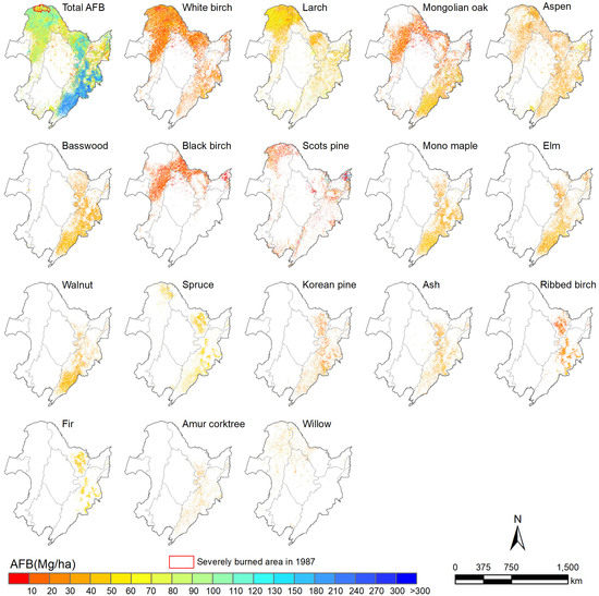
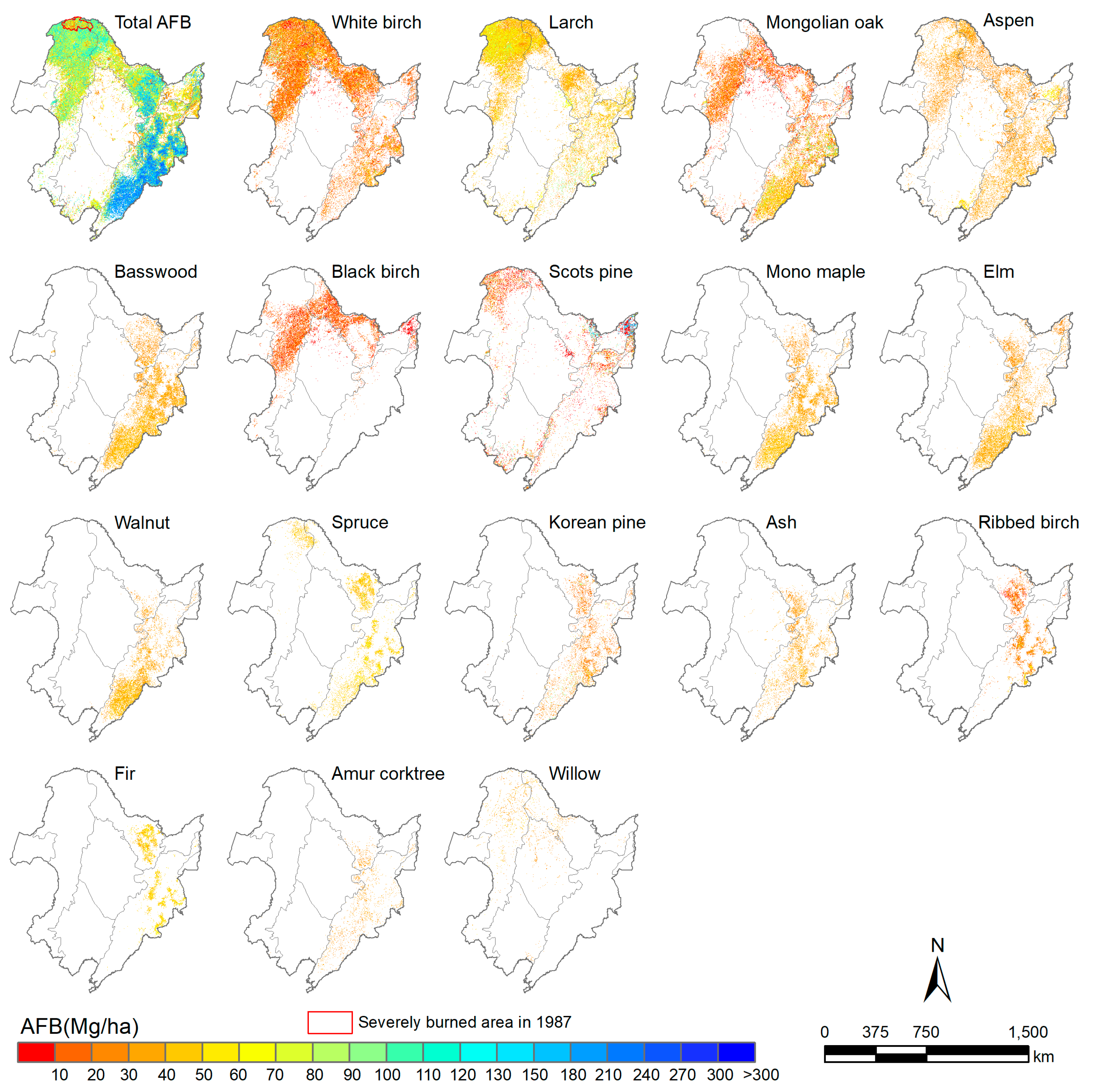
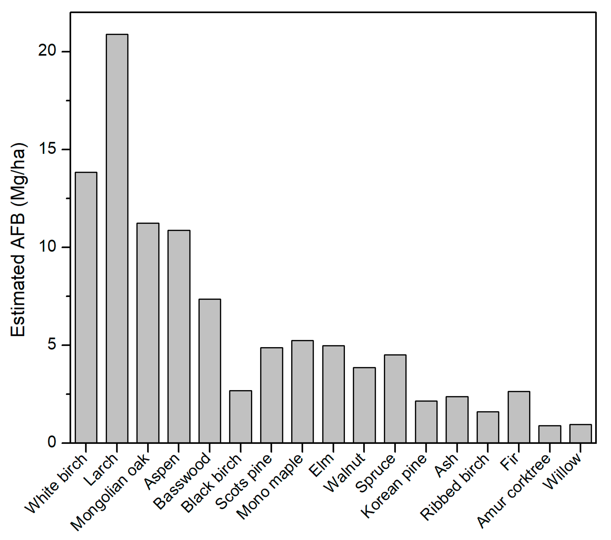
3.2. Species-Level AFB Estimation in Northeast China

The total AFB across the 17 species was mapped by summing the species-level AFB within each pixel. The average AFB of all the 17 species for entire Northeast China (excluding non-forest areas) was approximately 101.98 Mg/ha, and the standard deviation was 56.91 Mg/ha. Overall, the imputed total forest aboveground biomass in Northeast China was mainly distributed at ecoregion GKM, LKM and CM, and the average AFB in ecoregion CM was higher than that in ecoregion LKM and GKM (Figure 5). Ecoregion SNP, LHP, and SJP were all located in the plain area with the proportion of forest less than 5%, and the average AFB of these three ecoregions was low (Figure 5).
Larch had the largest AFB (20.88 Mg/ha), which was calculated by summing the biomass of all three larch species, indicating larch was the most dominant tree in Northeast China, followed by white birch (13.84 Mg/ha), although white birch had a broader distribution range than larch (Figure 5 and Figure 6). Mongolian oak and aspen were also widely distributed, with an average AFB of 11.23 Mg/ha and 10.87 Mg/ha, respectively. However, at the northern edge of ecoregion GKM, Mongolian oak was rare. Basswood, mono maple, elm, walnut, ash, and Korean pine were all mainly distributed in the southern LKM and CM, and their AFB decreased sequentially. Black birch (2.69 Mg/ha) was imputed mainly in the middle of ecoregion GKM, the north of LKM, and the north of SJP. Whereas Scots pine (4.88 Mg/ha) was mainly imputed in the northern GKM, CM, and SJP. Spruce (4.52 Mg/ha) was concentrated in the northeastern GKM, southern LKM, and the central CM. Ribbed birch and fir had similar distributions (concentrated in the southern LKM and the central CM), while the AFB of fir (2.65 Mg/ha) was higher than ribbed birch (1.62 Mg/ha). Amur corktree was sparsely distributed in the southern LKM and CM, and had the lowest AFB (0.91 Mg/ha). Willow also had very low AFB (0.96 Mg/ha) and was mostly imputed along rivers in ecoregion GKM, LKM and SNP.
The accuracy of the estimated total AFB improved substantially from the stand level to the ecotype level, the value of R2 increased from 0.63 to 0.92, and the value of RMSE decreased from 35.49 to 8.27 Mg/ha (Figure 7a,c). Although the value of the KS distance (0.12 vs. 0.05) was slightly higher at the ecotype level than that at the stand level, a higher P value (0.79 vs. 0) for KS distance at the ecotype level revealed that the estimated and observed AFB ECDFs became more similar (Figure 7b,d). For areas with limited forest stand polygons, validation at the 143 sample plots showed good accuracy, with R2, RMSE, KS distance and P value results of 0.76, 28.36 Mg/ha, 0.1 and 0.41, respectively (Figure 7e,f).
At the stand level, compared with the other species, the estimated species-level AFB for larch, fir, and willow had relatively higher accuracy (R2 = 0.56, 0.54, 0.51, respectively) (Figure S1) [47]. The KS statistic metrics indicated the ECDFs between the estimated and observed species-level AFB at the stand level for all the 17 species were significantly different with low P value (P = 0; Figure S2). The estimated AFB accuracy of most species (R2 = 0.77–0.98) except for willow and Scots pine (R2 = 0.55, 0.62, respectively) was significantly improved from the stand level to the ecotype level (Figure S3). At the ecotype level, the ECDFs between the observed and estimated species-level AFB became similar for all species with smaller KS distance (0.04–0.37) and higher P value (P ≈ 1; Figure S4).

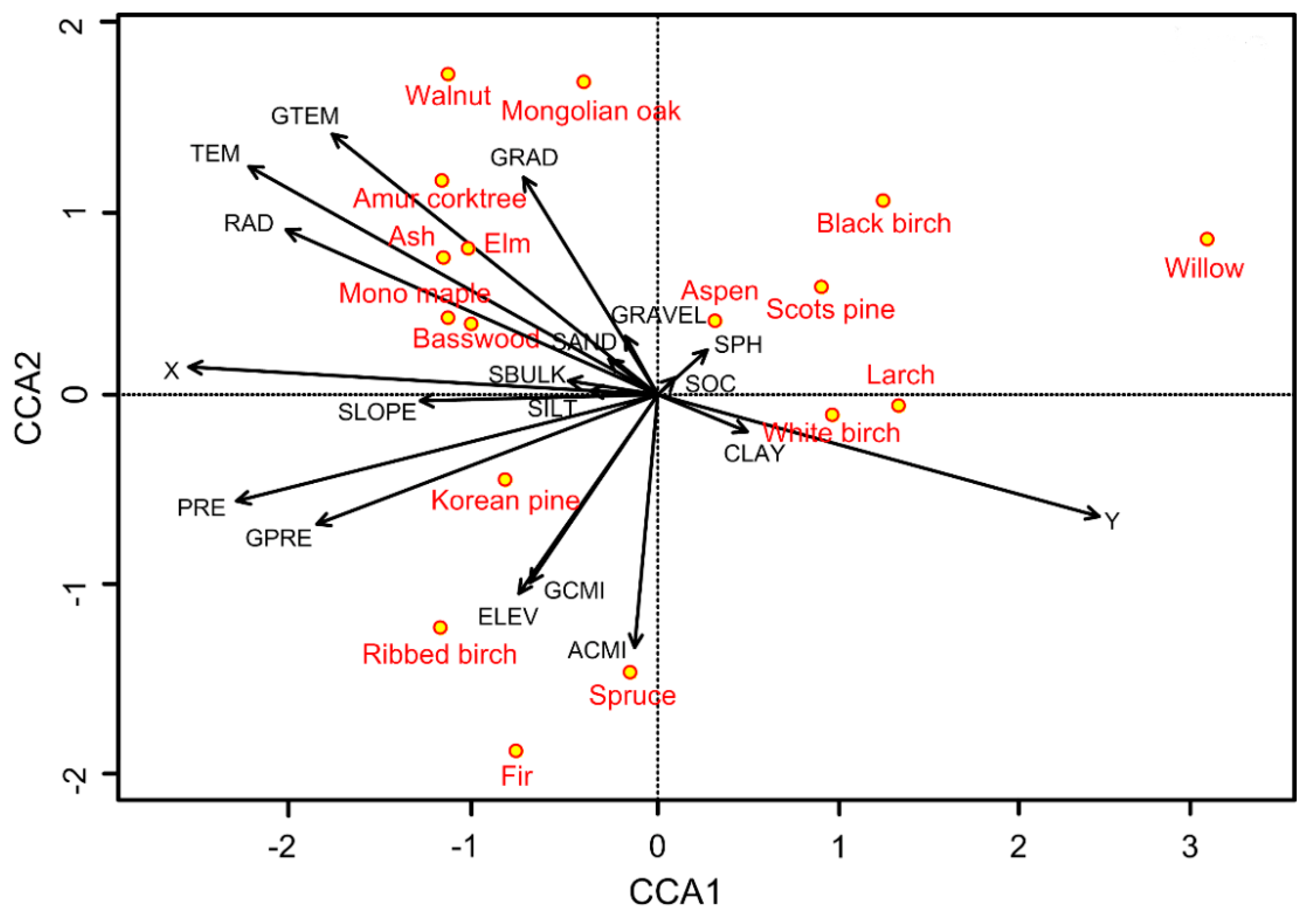
3.3. Relationship between Environmental Variables and Species-Level AFB

Environmental variables such as climate and topography variables had strong relationships with species-level AFB (Figure 8). For example, precipitation, elevation, and climate moisture index was positively correlated with the AFB of fir, spruce, ribbed birch, and Korean pine with strong correlation, but had a negative correlation with aspen, Scots pine and black birch. Temperature, radiation and slope were positively correlated with the AFB of mono maple, basswood, ash, elm, Amur corktree, walnut and Mongolian oak, but negatively correlated with larch and white birch. Mean annual climate variables (PRE, ACMI, TEM, and RAD) had stronger effects on the species-level AFB than the mean growing season variables (GPRE, GACMI, GTEM, and GRAD). The X and Y coordinates also strongly associated with species-level AFB, especially for willow. Compared with other environmental variables, soil variables contributed less to the species-level AFB.

4. Discussion

4.1. Selection of Optimal Distance Metric, k value and MODIS Imagery

RF-based kNN models produced the best results overall in our study. This may be because the RF distance metric is sufficient to process highly dimensional data and highly correlated predictor variables [17]. The performance of the MSN-based kNN model was similar to that of the RF-based kNN model, but its execution efficiency was higher. Therefore, it is worthwhile to consider using an MSN distance metric for large-scale biomass imputation rather than an RF distance metric to reduce the computational intensity. As the k value increased, the changing trend of T and GRMSD values in our study was the same as the results of Beaudoin et al. [16] and Zhang et al. [22]. Selection of optimal k value was the balance between covariance structure and imputation accuracy [12] and varied with different mapping applications. Different from the selection (k = 6) of Zhang et al. [22], in our study, k = 7 was selected, which could maintain the stable covariance structure of species composition. Zhang et al. [22] selected the single-month MODIS imagery for June as predictors. However, our results indicated that use of single-month MODIS imagery for September had the highest accuracy among the six selected months. The differences between our results and Zhang et al. [22] could be due to our study area spanning from temperate forests to boreal forests, and September imagery could best capture the differences in spectral reflectance among species that result from leaf senescence [48]. Our results suggest that the optimal kNN model selected by Zhang et al. [22] was not the optimal model for species-level biomass imputation for entire Northeast China, which confirms the necessity of selecting kNN models on a case-by-case basis [13].

4.2. Environmental Factors and Species Distribution

Environmental variables showed a major effect on the imputation of species-level AFB (Figure 8) because they were strongly correlated with the spatial patterns of tree species (Figure 5). Larch and white birch have high tolerance to low temperature [49], and are therefore distributed most widely in the northern part of our study region. The AFB of larch is commonly higher than white birch because it is a late-successional species compared to white birch [50]. Aspen has more limited distribution than white birch since it requires warmer temperatures and higher soil fertility [50]. Scots pine has a high tolerance of drought and low temperatures [51], and consequently is mainly distributed on sunny slopes and ridges in the northern edge GKM. The distribution of Mongolian oak and black birch in ecoregion GKM and LKM are similar since they have similar ecological niches [50]. Compared to black birch, Mongolian oak has a wider range of adaptation to environmental conditions, thus, Mongolian oak has a wider distribution and the AFB of Mongolian oak is obviously higher than black birch. Spruce and fir grow under cold environments [52], and therefore, they are mainly mapped in areas of relatively high elevation. Korean pine, ribbed birch, mono maple, basswood, ash, elm, Amur corktree, and walnut are most abundant in warmer ecoregions (i.e., LKM and CM), because they require sufficient humidity and heat to survive [53,54].
The spatial distribution of species-level AFB from our imputation results showed species composition similar to each ecoregion delineated by Zheng et al. [24]. Therefore, our imputation results provided support for the division of their ecoregions. Specifically, Zheng et al. [24] defined the ecoregion GKM as a deciduous-coniferous forest region, in which larch was the most dominant coniferous species with a small amount of Scots pine and spruce, and the main broadleaved tree species included white birch, Mongolian oak and aspen. Ecoregions LKM and CM were defined as coniferous and broadleaved mixed forest. Compared to GKM, ecoregions LKM and CM had similar species composition, including more coniferous species (e.g., Korean pine, fir) and broadleaved species (e.g., basswood, mono maple, elm, walnut, ash). The ecoregions SJP, SNP, LHP and HBP were defined as plain or plateau, with few tree species. The imputed species-level AFB also captured the forest regions affected by large disturbances. For example, the forests in the northernmost GKM were severely burned in 1987 [50], and thus, the total aboveground forest biomass in this region was obviously lower than other regions (Figure 5).

4.3. Imputation Accuracy and Limitations

Results from our study indicated that the total forest biomass of all species in the ecoregion CM was the largest, followed by that in ecoregion LKM and GKM, which were consistent with the biomass distribution of previous studies also conducted in Northeast China [23,55]. Results in our study showed the average AFB and total AFB carbon stock (multiplying by a standard factor of 0.5 to convert forest biomass to forest carbon stock) [56] in Northeast China was 101.98 Mg/ha and 2.51 Pg C, respectively. These results were higher than those estimated by Zhang et al. [23] in Northeast China (average AFB: 93.02 Mg/ha; total AFB carbon stock: 1.55 Pg C). The higher total AFB carbon stock in our study was most likely due to the definition of the forest as pixels with tree cover over 10%, lower than the 30% threshold defined by Zhang et al. [23], resulting in larger forest areas, and therefore an increase of the forest carbon stock [2]. In contrast, the total AFB carbon stock from our results was consistent with the value of 2.571 ± 0.075 Pg C estimated by Zhang et al. [55] for Northeast China, which also defined forest by a 10% threshold.
At the stand level, our imputation accuracy of total AFB (R2 = 0.63) was comparable or more accurate to the results of published studies (R2 = 0.43–0.69) [16,23,57], that integrated field plots and MODIS data for biomass mapping in Northeast China and Canada. Species-level AFB accuracy (R2 = 0.14–0.56) was more accurate than the results by Zhang et al. [22] (R2 = 0.01–0.47). These comparisons indicated that our estimation results had a relatively reliable accuracy and the optimal model developed for the whole Northeast China in this study could effectively identify species-level biomass in multiple constituent ecoregions. Some species (e.g., Amur corktree and walnut) had lower accuracy at the stand level, which may be due to their limited sample distribution. Each ecotype contained relatively homogeneous temperature, humidity, soil, topography, and forest type. Within each ecotype, the tree species heterogeneity was reduced and the composition and structure of the species were specific to ecotype [58]. Thus, at the ecotype level, the imputation accuracy of both total AFB and species-level AFB had significant improvement except for willow and Scots pine. The lesser accuracy improvement for willow and Scots pine might be because their inventory data were relatively concentrated and distributed on fewer ecotypes. One solution to reduce the variances of inventory data distribution is to obtain sufficient field sample data evenly distributed across the ecotypes and within each ecotype. In order to obtain sufficient field sample data, more field inventories across different ecotypes and integrating lidar-based metrics and field sample data may be necessary. The lidar footprints distribute evenly and widely, and thus, the derived forest attributes in these footprints could be better used to impute the species-level AFB [2].
Though the inventory data were abundant in the three well-investigated forest regions and could well represent the forest composition in Northeast China, lack of inventory data in the other forest areas may lead to overestimations or underestimations of the species-level biomass. There are also limitations in the methodology and input parameters (e.g., MODIS variables). For example, the imputation results of the species-level aboveground forest biomass in our study indicated small values were often overestimated and large values were underestimated. This pattern is a typical feature of the kNN imputation method [59] and may also be caused by the spectral saturation of optical MODIS data in the forests with dense canopy cover [16]. Besides the saturation effect, the coarse spatial resolution (250 m) of MODIS data may also affect the estimation accuracy of the biomass, which will increase the possibility for the mismatch between forest stand polygon and pixels, especially along polygon boundaries. Due to the irregular boundaries of forest stand polygons, there would always be a spatial mismatch between the forest stand polygons and MODIS pixels even using remote sensing data with a finer spatial resolution [60]. In our study, when more than one raster pixel falls into one forest stand polygon, we extracted the pixel value of each stand polygon by averaging the values of the raster pixels with >50% stand cover to reduce contingency in the comparison with the stand-level attributes.

5. Conclusions

This study represents the first effort to map species-level aboveground forest biomass for the entirety of Northeast China. The biomass maps of the 17 species generated from this work are the basic prerequisites for regional-level ecological modelling and assessment in Northeast China. By integrating MODIS multispectral and environmental variables with forest inventory data, the optimal kNN model selected in this study provided a cost-effective means for such an effort. Among the six distance metrics, random forest presented the highest accuracy to impute the species-level aboveground forest biomass. The use of all six-months of MODIS data did not significantly improve the imputation accuracy compared to the use of single-month MODIS data for September. Among the 15 k values (1–15), k = 7 as the input parameter of the kNN model showed the best accuracy. Larch was the most dominant species in Northeast China, followed by white birch. The biomass of willow and Amur corktree was very low due to their limited distribution over the study area. Overall, the aboveground forest biomass in the Greater Khingan Mountains was lower than that in the Lesser Khingan and Changbai Mountains. Accuracy of the results improved obviously from the stand level up to the ecotype level, therefore our results are more suitable to apply to forest ecosystem models (e.g., LINKAGES) which require species-level attributes at the ecotype scale. Our mapped wall-to-wall species-level biomass can also be used to initialize the forest landscape models (e.g., LANDIS) to simulate changes in tree species composition. The spatial pattern of species-level aboveground forest biomass presented here could also capture the forest regions influenced by disturbance (e.g., fire or harvest). However, this study presented the maps of species-level aboveground forest biomass in Northeast China for only one year (2000). In order to better assess the influence of disturbance and climate change on forests, the temporal variation of species-level aboveground forest biomass should be further studied.

Supplementary Materials

The following are available online at https://www.mdpi.com/2072-4292/11/17/2005/s1, Figure S1: Scatter plot between the observed and the estimated AFB for 17 species separately based on the testing data at the stand level, Figure S2: Cumulative distribution functions of the observed and the estimated AFB for 17 species separately based on the testing data at the stand level, Figure S3: Scatter plot between the observed and the estimated AFB for 17 species separately based on the testing data at the ecotype level, Figure S4: Cumulative distribution functions of the observed and the estimated AFB for 17 species separately based on the testing data at the ecotype level.

Author Contributions

Conceptualization, Y.F. and H.S.H.; Methodology, Y.F., T.J.H. and P.D.H.; Formal analysis, Y.F., T.J.H. and P.D.H.; Writing—original draft, Y.F.; Writing—review & editing, T.J.H., P.D.H., Z.Z. and D.R.L.; Funding acquisition, H.S.H.

Funding

This research was funded by the National Key Research and Development Program of China (Grant number 2017YFA0604403 and 2016YFA0602301), University of Missouri GIS Mission Enhancement Program and National Biologic Carbon Sequestration Assessment Program under the U.S. Geological Survey (USGS) Climate and Land Use Mission Area.

Acknowledgments

We gratefully acknowledge Shengwei Zong for materials donations and Qinglong Zhang for technical support. Any use of trade, firm, or product names is for descriptive purposes only and does not imply endorsement by the U.S. Government.

Conflicts of Interest

The authors declare no conflict of interest.

References

  1. Li, L.; Guo, Q.; Tao, S.; Kelly, M.; Xu, G. Lidar with multi-temporal MODIS provide a means to upscale predictions of forest biomass. ISPRS J. Photogramm. Remote Sens. 2015, 102, 198–208. [Google Scholar] [CrossRef]
  2. Su, Y.; Guo, Q.; Xue, B.; Hu, T.; Alvarez, O.; Tao, S.; Fang, J. Spatial distribution of forest aboveground biomass in China: Estimation through combination of spaceborne lidar, optical imagery, and forest inventory data. Remote Sens. Environ. 2016, 173, 187–199. [Google Scholar] [CrossRef] [Green Version]
  3. Zolkos, S.; Goetz, S.; Dubayah, R. A meta-analysis of terrestrial aboveground biomass estimation using lidar remote sensing. Remote Sens. Environ. 2013, 128, 289–298. [Google Scholar] [CrossRef]
  4. He, H.S. Forest landscape models: Definitions, characterization, and classification. For. Ecol. Manag. 2008, 254, 484–498. [Google Scholar] [CrossRef]
  5. Duveneck, M.J.; Thompson, J.R.; Wilson, B.T. An imputed forest composition map for New England screened by species range boundaries. For. Ecol. Manag. 2015, 347, 107–115. [Google Scholar] [CrossRef]
  6. Zald, H.S.; Wulder, M.A.; White, J.C.; Hilker, T.; Hermosilla, T.; Hobart, G.W.; Coops, N.C. Integrating Landsat pixel composites and change metrics with lidar plots to predictively map forest structure and aboveground biomass in Saskatchewan, Canada. Remote Sens. Environ. 2016, 176, 188–201. [Google Scholar] [CrossRef] [Green Version]
  7. Wilson, B.T.; Lister, A.J.; Riemann, R.I. A nearest-neighbor imputation approach to mapping tree species over large areas using forest inventory plots and moderate resolution raster data. For. Ecol. Manag. 2012, 271, 182–198. [Google Scholar] [CrossRef]
  8. Zhang, G.; Ganguly, S.; Nemani, R.R.; White, M.A.; Milesi, C.; Hashimoto, H.; Wang, W.; Saatchi, S.; Yu, Y.; Myneni, R.B. Estimation of forest aboveground biomass in California using canopy height and leaf area index estimated from satellite data. Remote Sens. Environ. 2014, 151, 44–56. [Google Scholar] [CrossRef]
  9. Hermosilla, T.; Wulder, M.A.; White, J.C.; Coops, N.C.; Hobart, G.W. An integrated Landsat time series protocol for change detection and generation of annual gap-free surface reflectance composites. Remote Sens. Environ. 2015, 158, 220–234. [Google Scholar] [CrossRef]
  10. Ohmann, J.L.; Gregory, M.J. Predictive mapping of forest composition and structure with direct gradient analysis and nearest-neighbor imputation in coastal Oregon, USA. Can. J. For. Res. 2002, 32, 725–741. [Google Scholar] [CrossRef]
  11. Tomppo, E.; Olsson, H.; Ståhl, G.; Nilsson, M.; Hagner, O.; Katila, M. Combining national forest inventory field plots and remote sensing data for forest databases. Remote Sens. Environ. 2008, 112, 1982–1999. [Google Scholar] [CrossRef]
  12. McRoberts, R.E. Estimating forest attribute parameters for small areas using nearest neighbors techniques. For. Ecol. Manag. 2012, 272, 3–12. [Google Scholar] [CrossRef]
  13. Eskelson, B.N.; Temesgen, H.; Lemay, V.; Barrett, T.M.; Crookston, N.L.; Hudak, A.T. The roles of nearest neighbor methods in imputing missing data in forest inventory and monitoring databases. Scand. J. For. Res. 2009, 24, 235–246. [Google Scholar] [CrossRef] [Green Version]
  14. Vauhkonen, J.; Korpela, I.; Maltamo, M.; Tokola, T. Imputation of single-tree attributes using airborne laser scanning-based height, intensity, and alpha shape metrics. Remote Sens. Environ. 2010, 114, 1263–1276. [Google Scholar] [CrossRef]
  15. Brosofske, K.D.; Froese, R.E.; Falkowski, M.J.; Banskota, A. A review of methods for mapping and prediction of inventory attributes for operational forest management. For. Sci. 2013, 60, 733–756. [Google Scholar] [CrossRef]
  16. Beaudoin, A.; Bernier, P.; Guindon, L.; Villemaire, P.; Guo, X.; Stinson, G.; Bergeron, T.; Magnussen, S.; Hall, R. Mapping attributes of Canada’s forests at moderate resolution through kNN and MODIS imagery. Can. J. For. Res. 2014, 44, 521–532. [Google Scholar] [CrossRef]
  17. Hudak, A.T.; Crookston, N.L.; Evans, J.S.; Hall, D.E.; Falkowski, M.J. Nearest neighbor imputation of species-level, plot-scale forest structure attributes from lidar data. Remote Sens. Environ. 2008, 112, 2232–2245. [Google Scholar] [CrossRef]
  18. Moeur, M.; Stage, A.R. Most similar neighbor: An improved sampling inference procedure for natural resource planning. For. Sci. 1995, 41, 337–359. [Google Scholar]
  19. Crookston, N.L.; Finley, A.O. Yaimpute: An R package for kNN imputation. J. Stat. Softw. 2008, 23. [Google Scholar] [CrossRef]
  20. Falkowski, M.J.; Hudak, A.T.; Crookston, N.L.; Gessler, P.E.; Uebler, E.H.; Smith, A.M. Landscape-scale parameterization of a tree-level forest growth model: A k-nearest neighbor imputation approach incorporating lidar data. Can. J. For. Res. 2010, 40, 184–199. [Google Scholar] [CrossRef]
  21. Ohmann, J.L.; Gregory, M.J.; Henderson, E.B.; Roberts, H.M. Mapping gradients of community composition with nearest-neighbour imputation: Extending plot data for landscape analysis. J. Veg. Sci. 2011, 22, 660–676. [Google Scholar] [CrossRef]
  22. Zhang, Q.; He, H.S.; Liang, Y.; Hawbaker, T.J.; Henne, P.D.; Liu, J.; Huang, S.; Wu, Z.; Huang, C. Integrating forest inventory data and MODIS data to map species-level biomass in Chinese boreal forests. Can. J. For. Res. 2018, 48, 461–479. [Google Scholar] [CrossRef]
  23. Zhang, Y.; Liang, S.; Sun, G. Forest biomass mapping of northeastern China using GLAS and MODIS data. IEEE J. Sel. Top. Appl. Earth Obs. Remote Sens. 2014, 7, 140–152. [Google Scholar] [CrossRef]
  24. Zheng, D.; Yang, Q.; Wu, S.; Li, B. Study on Eco-geographic System of China; The Commercial Press: Beijing, China, 2008. (In Chinses) [Google Scholar]
  25. Chi, H.; Sun, G.; Huang, J.; Guo, Z.; Ni, W.; Fu, A. National forest aboveground biomass mapping from ICESat/GLAS data and MODIS imagery in China. Remote Sens. 2015, 7, 5534–5564. [Google Scholar] [CrossRef]
  26. Fang, J.-Y.; Wang, G.G.; Liu, G.-H.; Xu, S.-L. Forest biomass of China: An estimate based on the biomass–volume relationship. Ecol. Appl. 1998, 8, 1084–1091. [Google Scholar]
  27. Wang, X.; Fang, J.; Zhu, B. Forest biomass and root–shoot allocation in Northeast China. For. Ecol. Manag. 2008, 255, 4007–4020. [Google Scholar] [CrossRef]
  28. Ni, J.; Zhang, X.-s.; Scurlock, J.M. Synthesis and analysis of biomass and net primary productivity in Chinese forests. Ann. For. Sci. 2001, 58, 351–384. [Google Scholar] [CrossRef]
  29. Schmitt, C.B.; Burgess, N.D.; Coad, L.; Belokurov, A.; Besançon, C.; Boisrobert, L.; Campbell, A.; Fish, L.; Gliddon, D.; Humphries, K. Global analysis of the protection status of the world’s forests. Biol. Conserv. 2009, 142, 2122–2130. [Google Scholar] [CrossRef]
  30. Tucker, C.J. Red and photographic infrared linear combinations for monitoring vegetation. Remote Sens. Environ. 1979, 8, 127–150. [Google Scholar] [CrossRef] [Green Version]
  31. Jordan, C.F. Derivation of leaf-area index from quality of light on the forest floor. Ecology 1969, 50, 663–666. [Google Scholar] [CrossRef]
  32. Huete, A.; Didan, K.; Miura, T.; Rodriguez, E.P.; Gao, X.; Ferreira, L.G. Overview of the radiometric and biophysical performance of the MODIS vegetation indices. Remote Sens. Environ. 2002, 83, 195–213. [Google Scholar] [CrossRef]
  33. Qi, J.; Chehbouni, A.; Huete, A.; Kerr, Y.; Sorooshian, S. A modified soil adjusted vegetation index. Remote Sens. Environ. 1994, 48, 119–126. [Google Scholar] [CrossRef]
  34. Gitelson, A.A.; Kaufman, Y.J.; Stark, R.; Rundquist, D. Novel algorithms for remote estimation of vegetation fraction. Remote Sens. Environ. 2002, 80, 76–87. [Google Scholar] [CrossRef] [Green Version]
  35. Gao, B.-C. NDWI—A normalized difference water index for remote sensing of vegetation liquid water from space. Remote Sens. Environ. 1996, 58, 257–266. [Google Scholar] [CrossRef]
  36. Hunt Jr, E.R.; Rock, B.N. Detection of changes in leaf water content using near-and middle-infrared reflectances. Remote Sens. Environ. 1989, 30, 43–54. [Google Scholar]
  37. Huete, A.R. A soil-adjusted vegetation index (SAVI). Remote Sens. Environ. 1988, 25, 295–309. [Google Scholar] [CrossRef]
  38. Pinty, B.; Verstraete, M. Gemi: A non-linear index to monitor global vegetation from satellites. Vegetatio 1992, 101, 15–20. [Google Scholar] [CrossRef]
  39. Gitelson, A.A. Wide dynamic range vegetation index for remote quantification of biophysical characteristics of vegetation. J. Plant Physiol. 2004, 161, 165–173. [Google Scholar] [CrossRef]
  40. Zhang, N.; Hong, Y.; Qin, Q.; Zhu, L. Evaluation of the visible and shortwave infrared drought index in China. Int. J. Disaster Risk Sci. 2013, 4, 68–76. [Google Scholar] [CrossRef] [Green Version]
  41. Fu, Y.; He, H.S.; Zhao, J.; Larsen, D.R.; Zhang, H.; Sunde, M.G.; Duan, S. Climate and spring phenology effects on autumn phenology in the Greater Khingan Mountains, northeastern China. Remote Sens. 2018, 10, 449. [Google Scholar] [CrossRef]
  42. FAO; IIASA; ISRIC; ISSCAS; JRC. Harmonized World Soil Database (Version 1.2); FAO: Rome, Italy; IIASA: Laxenburg, Austria, 2012. [Google Scholar]
  43. Crookston, N.L.; Finley, A.O. Yaimpute: Nearest Neighbor Observation Imputation and Evaluation Tools. R Package Version 1.0-30. 2018. Available online: http://CRAN.R-project.org/package=yaImpute (accessed on 1 July 2019).
  44. Zhang, Y.; He, H.S.; Dijak, W.D.; Yang, J.; Shifley, S.R.; Palik, B.J. Integration of satellite imagery and forest inventory in mapping dominant and associated species at a regional scale. Environ. Manage. 2009, 44, 312–323. [Google Scholar] [CrossRef] [PubMed]
  45. Riemann, R.; Wilson, B.T.; Lister, A.; Parks, S. An effective assessment protocol for continuous geospatial datasets of forest characteristics using USFS forest inventory and analysis (FIA) data. Remote Sens. Environ. 2010, 114, 2337–2352. [Google Scholar] [CrossRef]
  46. Lopes, R.H.; Reid, I.; Hobson, P.R. The two-dimensional Kolmogorov-Smirnov test. In Proceedings of the XI International Workshop on Advanced Computing and Analysis Techniques in Physics Research, Amsterdam, The Netherlands, 23–27 April 2007; pp. 196–206. [Google Scholar]
  47. Fu, Y.; He, H.S.; Hawbaker, T.J.; Henne, P.D.; Zhu, Z.; Larsen, D.R. Data Release For: Evaluating k-Nearest Neighbor (kNN) Imputation Models for Species-Level Aboveground Forest Biomass Mapping in Northeast China. U.S. Geological Survey Data Release. 2019. Available online: https://doi.org/10.5066/P9MOB5E3 (accessed on 1 July 2019).
  48. Yu, X.-f.; Zhuang, D.-f. Monitoring forest phenophases of Northeast China based on MODIS NDVI data. Resour. Sci. 2006, 28, 111–117. [Google Scholar]
  49. Mao, Q.; Watanabe, M.; Koike, T. Growth characteristics of two promising tree species for afforestation, birch and larch in the northeastern part of Asia. Eurasian J. For. Res. 2010, 13, 69–76. [Google Scholar]
  50. Xu, H. Forest in Great Xing’an Mountains of China; Science Press: Beijing, China, 1998. (In Chinese) [Google Scholar]
  51. Zhu, J.; Kang, H.; Tan, H.; Xu, M. Effects of drought stresses induced by polyethylene glycol on germination of Pinus sylvestris var. mongolica seeds from natural and plantation forests on sandy land. J. For. Res. 2006, 11, 319–328. [Google Scholar] [CrossRef]
  52. Yu, D.; Wang, Q.; Wang, Y.; Zhou, W.; Ding, H.; Fang, X.; Jiang, S.; Dai, L. Climatic effects on radial growth of major tree species on Changbai Mountain. Ann. For. Sci. 2011, 68, 921. [Google Scholar] [CrossRef]
  53. Xiao-Ying, W.; Chun-Yu, Z.; Qing-Yu, J. Impacts of climate change on forest ecosystems in Northeast China. Adv. Clim. Chang. Res. 2013, 4, 230–241. [Google Scholar] [CrossRef]
  54. Ma, J.; Hu, Y.; Bu, R.; Chang, Y.; Deng, H.; Qin, Q. Predicting impacts of climate change on the aboveground carbon sequestration rate of a temperate forest in northeastern China. PLoS ONE 2014, 9, e96157. [Google Scholar] [CrossRef]
  55. Zhang, Y.; Liang, S. Changes in forest biomass and linkage to climate and forest disturbances over northeastern China. Glob. Chang. Biol. 2014, 20, 2596–2606. [Google Scholar] [CrossRef]
  56. Saatchi, S.S.; Harris, N.L.; Brown, S.; Lefsky, M.; Mitchard, E.T.; Salas, W.; Zutta, B.R.; Buermann, W.; Lewis, S.L.; Hagen, S. Benchmark map of forest carbon stocks in tropical regions across three continents. Proc. Natl. Acad. Sci. 2011, 108, 9899–9904. [Google Scholar] [CrossRef] [Green Version]
  57. Ni, X.; Cao, C.; Zhou, Y.; Ding, L.; Choi, S.; Shi, Y.; Park, T.; Fu, X.; Hu, H.; Wang, X. Estimation of forest biomass patterns across Northeast China based on allometric scale relationship. Forests 2017, 8, 288. [Google Scholar] [CrossRef]
  58. He, H.S.; Mladenoff, D.J.; Radeloff, V.C.; Crow, T.R. Integration of GIS data and classified satellite imagery for regional forest assessment. Ecol. Appl. 1998, 8, 1072–1083. [Google Scholar] [CrossRef]
  59. Magnussen, S.; Tomppo, E.; McRoberts, R.E. A model-assisted k-nearest neighbour approach to remove extrapolation bias. Scand. J. For. Res. 2010, 25, 174–184. [Google Scholar] [CrossRef]
  60. Matasci, G.; Hermosilla, T.; Wulder, M.A.; White, J.C.; Coops, N.C.; Hobart, G.W.; Zald, H.S. Large-area mapping of Canadian boreal forest cover, height, biomass and other structural attributes using Landsat composites and lidar plots. Remote Sens. Environ. 2018, 209, 90–106. [Google Scholar] [CrossRef]
Figure 1. Seven ecoregions, forest cover fraction and forest inventory data distribution in Northeast China.
Remotesensing 11 02005 g001
Figure 2. The processing flow of species-level AFB imputation.
Remotesensing 11 02005 g002
Figure 3. Multivariate goodness of fit criterion (T) curves vs. k based on six distance metrics and seven sets of predictors. Larger T values mean better model performance.
Remotesensing 11 02005 g003
Figure 4. Multivariate generalized root mean squared distance (GRMSD) curves vs. k based on six distance metrics and seven sets of predictors. Larger GRMSD values mean worse model performance.
Remotesensing 11 02005 g004
Figure 5. Maps of total AFB and species-level AFB in Northeast China.
Remotesensing 11 02005 g005
Figure 6. Mean values of the estimated species-level AFB in Northeast China.
Remotesensing 11 02005 g006
Figure 7. (a) Scatter plot between the observed and the estimated total AFB at the stand level; (b) cumulative distribution functions of the observed and the estimated total AFB at the stand level; (c) scatter plot between the observed and the estimated total AFB at the ecotype level; (d) cumulative distribution functions of the observed and the estimated total AFB at the ecotype level; (e) scatter plot between the observed and the estimated total AFB at the sample plots; (f) cumulative distribution functions of the observed and the estimated total AFB at the sample plots. Note that the dotted line is the 1:1 line.
Remotesensing 11 02005 g007
Figure 8. CCA biplots showing associations between 17 species AFB and the significant environmental variables (P < 0.01). Species placement is marked with a red circle filled with yellow. Black arrows indicate the direction and relative importance of the environmental variables.
Remotesensing 11 02005 g008
Table 1. Candidate predictor variables used in kNN imputation models. The growing season was defined as May to October.
Category and SubcategoryLabelDescription
Spectral
Spectral bandsb1Red, 620–670 nm
b2Short wave near-infrared, 841–876 nm
b3Blue, 459–479 nm
b4Green, 545–565 nm
b5Long wave near-infrared, 1230–1250 nm
b6Long wave near-infrared, 1628–1652 nm
b7Long wave near-infrared, 2105–2155 nm
Spectral indicesNDVI ( b 2 b 1 ) / ( b 2 + b 1 ) [30]
RVI b 2 / b 1 [31]
EVI 2.5 ( b 2 b 1 ) / ( b 2 + 6 b 1 7.5 b 3 + 1 ) [32]
MSAVI b 2 + 0.5 0.5 2 b 2 + 1 2 8 ( b 2 b 1 ) [33]
VARI ( b 4 b 1 ) / ( b 4 + b 1 b 3 ) [34]
NDWI ( b 2 b 5 ) / ( b 2 + b 5 ) [35]
NDIIb6 ( b 2 b 6 ) / ( b 2 + b 6 ) [36]
NDIIb7 ( b 2 b 7 ) / ( b 2 + b 7 ) [36]
SAVI 1.5 ( b 2 b 1 ) / ( b 2 + b 1 + 0.5 ) [37]
GEMI n ( 1 0.25 n ) ( b 1 0.125 ) / ( 1 b 1 )
n = ( 2 ( b 2 2 b 1 2 ) + 1.5 b 2 + 0.5 b 1 ) / ( b 2 + b 1 + 0.5 ) [38]
WDVI ( 0.2 b 2 b 1 ) / ( 0.2 b 2 + b 1 ) [39]
MSI b 6 / b 2 [36]
SWCI ( b 6 b 7 ) / ( b 6 + b 7 ) [40]
TopographicELEVElevation (m)
SLOPESlope (°)
COSASPCosine transformation of aspect
Climatic
TemperatureTEMMean annual temperature (°C)
GTEMMean temperature during the growing season (°C)
PrecipitationPREMean annual precipitation (mm)
GPREMean precipitation during the growing season (mm)
MoistureACMIMean annual climate moisture index (annual precipitation minus annual potential evapotranspiration) (mm) [16]
GCMIMean climate moisture index during the growing season (mm)
RadiationRADMean annual radiation (W/m2)
GRADMean radiation during the growing season (W/m2)
SoilSBULKBulk of soil (kg/dm3)
SPHPH of soil
GRAVELContent (%) of gravel
SANDContent (%) of sand
SILTContent (%) of silt
CLAYContent (%) of clay
SOCContent (%) of soil organic carbon
LocationXCoordinate x of each raster cell center (m)
YCoordinate y of each raster cell center (m)

