Forest Canopy Height and Gaps from Multiangular BRDF, Assessed with Airborne LiDAR Data

Abstract

Both vegetation multi-angular and LiDAR (light detection and ranging) remote sensing data are indirectly and directly linked with 3D vegetation structure parameters, such as the tree height and vegetation gap fraction, which are critical elements in above-ground biomass and light profiles for photosynthesis estimation. LiDAR, particularly LiDAR using waveform data, provides accurate estimates of these structural parameters but suffers from not enough spatial samplings. Structural parameters retrieved from multiangular imaging data through the inversion of physical models have larger uncertainties. This study searches for an analytical approach to fuse LiDAR and multiangular data. We explore the relationships between vegetation structure parameters derived from airborne vegetation LiDAR data and multiangular data and present a new potential angle vegetation index to retrieve the tree height and gap fraction using multi-angular data in Howland Forest, Maine. The BRDF (bidirectional reflectance distribution factor) index named NDMM (normalized difference between the maximum and minimum reflectance) linearly increases with the tree height and decreases with the gap fraction. In addition, these relationships are also dependent on the wavelength, tree species, and stand density. The NDMM index performs better in conifer (R = 0.451 for tree height and R = 0.472 for the gap fraction using the near infrared band) than in deciduous and mixed forests. It is superior in sparse (R = 0.569 for tree height and R = 0.604 for the gap fraction using the near infrared band) compared to dense forest. Moreover, the NDMM index is more strongly related to tree height and the gap fraction at the near infrared band than at the three visible bands. This study sheds light on the possibility of using multiangular data to map vegetation’s structural parameters in larger regions for carbon cycle studies through the fusion of LiDAR and multiangular remote sensing data.

1. Introduction

Vertical and horizontal forest-structure information is essential for many aspects of global ecosystem studies. For example, the tree height and vegetation gap fraction are the key parameters used to calculate the above ground biomass. Biomass represents the carbon store of forest cover. The accurate assessment of the carbon storage of forest cover over large areas is essential to the quantitative measurement and modeling of the global carbon ecosystem. Three-dimensional forest-structure data represent the different successive stages of forest ecosystems and are good indicators of ecosystem processes, such as natural and anthropogenic disturbances. Further, more accurate knowledge of vertical foliage profiles is essential to obtaining an accurate estimate of light profiles for photosynthesis. In essence, forest-structure data are important for many ecosystem process studies. However, measuring the 3D canopy structure from the ground is difficult and time consuming. Remote estimation of vegetation-structure characteristics is an essential tool for advancing 3D vegetation-structure parameter estimation for many ecosystem modeling studies.

Over many remote sensing measurements, vegetation LiDAR (light detection and ranging) and multi-angular optical remote sensing measurements provide direct and indirect vegetation-structure measurements. The potential use of laser technology to measure tree canopy heights was first documented by Nelson [1]. Only recently has its potential use been recognized, with more and more airborne and spaceborne LiDAR and multi-angular data available. The global LiDAR data collected using the spaceborne-geoscience laser altimeter system (GLAS) (part of the ICESat mission with a 70 m footprint) are available [2]. Further, the airborne data collected by the laser vegetation imaging sensor (LVIS) (with a 25 m footprint) over several large areas are better used to characterize vegetation structures [3]. These data will soon provide vegetation-structure data on a global scale via ICESat measurements [4] or at large regional scales via LVIS measurements [5]. Further, many small-footprint LiDAR data, also called terrain LiDAR data, have been collected in many small regions. Many vegetation-structure parameters and ground elevations have been derived from canopy LiDAR data [6]. For example, canopy height is calculated as the distance between the first significant return above a threshold and the ground [7,8,9,10,11]. Airborne LiDAR is more suitable for measuring tree height than ground measurements, especially when the crown cannot be viewed clearly [12,13]. Moreover, the LiDAR-derived tree height and gap is used as a true value. Tree canopy size and gap are usually related to photosynthesis, nutrient cycling, energy transfer, and light transmission to the understory vegetation, and these properties affect tree growth. The canopy gap determines the laser echo energy and can be directly calculated by the cumulative laser return from the canopy to the height divided by the total returns from the canopy and the ground, and is adjusted by a ratio to account for the differences in the ground and canopy reflectance at the laser wavelength [14]. Both the canopy cover and canopy height are parameters describing horizontal and vertical foliage distribution, which provide not only the horizontal structure but also the vertical vegetation-structure data suitable for ecosystem studies.

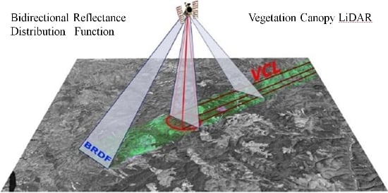
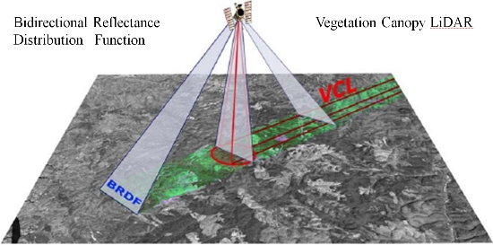
However, both the spaceborne and airborne LiDAR data can only accurately provide vegetation-structure information at sparse sampling points. Thus, there is a need to find a different, more conventional, remote sensing modality with more complete geographic coverage. Compared with traditional nadir-viewed remote sensing, a multiangular sensor can provide three-dimensional structural information of a forest via different directional observations. Multiangular remote sensing measures the shape of the bidirectional reflectance distribution factor (BRDF), which show links to the canopy’s structure [15,16,17,18]. Many models have been developed to link vegetation-structure parameters and BRDF [19,20]. However, multiangular remote sensing suffers from not being able to directly derive structural canopy measurements in the estimation of biomass without the inversion of these physical models. The geometric-optical BRDF model using spatial variance in single-view thematic mapper images has shown some early success in retrieval of the canopy cover, but biomass and forest-structure parameters were retrieved only with difficulty [21,22]. There have been some recent efforts to derive structural information using semi-physical BRDF models to better use advanced MODIS and multiangular imaging spectroradiometer (MISR) sensors on the current EOS-TERRA and AQUA platforms [23,24]. Chen, et al. [25,26] recently mapped horizontal foliage clumping using the anisotropic indexes, which are the normalized reflectance differences at hot-spot and cold-spot sampling directions. However, these structural data are not directly linked to the parameters important to biomass and vertical light profiles, and the hot-spot and cold-spot reflectance cannot usually be taken by multi-angular sensors, such as MODIS, MISR, and CHIRS(Compact High Resolution Imaging Spectrometer), because the hot-spot’s and cold-spot’s angles always change according to the imaging location and imaging time. Kimes, et al. [27] developed multivariate linear regression and neural network models to predict the LVIS forest energy height measurements from 28 airborne multiangular imaging spectroradiometer (AirMISR). However, the sensitive angles and bands of the models always change according to different study sites. A universal model or multiangular index without study site restrictions should be developed to retrieve vegetation’s structural parameters using BRDF data.

Taken together, these studies show that canopy structural information is contained in multiangular reflectance measurements, but structural parameters remain difficult to retrieve directly by the inversion of remotely sensed data, especially at coarse spatial scales. However, it is possible to develop a relationship between multiangular data and vegetation-structure parameters based on LiDAR data, using these relationships to map the vegetation-structure parameters from multiangular data. Both the airborne LVIS data and airborne multiangular imaging spectroradiometer (AirMISR) data were collected in several large regions at the same spatial scale for nearly the same period, which facilitated this kind of study. The major purpose of this study was to explore the relationships between vegetation-structure parameters and multiangular data via the anisotropic index, calculated based on the AirMISR data in a Howland conifer forest assessed with airborne LiDAR data.

2. Site Description and Data Sets

2.1. Howland Forest

The study site is Howland Forest, Maine, USA (45.17°N–45.26°N, 68.65°W–68.81°W). Both airborne LVIS and AirMISR sensors were flown into the Howland Forest during the summer of 2003. The natural stands in this northern hardwood boreal transitional forest consist of hemlock-spruce-fir, aspen-birch, and hemlock-hardwood mixtures. The tree species include quaking aspen, paper birch, eastern hemlock, red spruce, balsam fir, and red maple. Our focus plots are evenly distributed over the whole study area, which includes all the typical conifer forest stands in Howland. The true color composite AirMISR image collected in July 2003 and the typical forest type (see the description below) show the vegetation distribution in the study area (Figure 1). We selected three kinds of stands with a size of 5 × 5 pixels: low forest stands (red squares), high and sparse forest stands (blue squares), and high and dense forest stands (yellow squares) based on high spatial resolution images from Google earth. The forest includes five typical forests: conifer, deciduous, mixed forest, shrubland, and wetland, and the natural stands in this northern hardwood-boreal transitional forest consist of hemlock-spruce-fir, aspen-birch, and hemlock-hardwood mixtures [28].

2.2. AirMISR Data in Howland Forest

The AirMISR is an airborne instrument for obtaining multiangular imagery, similar to that of the satellite-borne, multi-angle imaging spectroradiometer (MISR), a global, multispectral, multiangular imager aboard the Terra platform. AirMISR flew on the NASA-owned ER-2 aircraft. MISR employs nine discrete cameras pointed at fixed angles; these cameras imaged Earth at 26.1, 45.6, 60.0, and 70.5 degrees forward and aftward from the local vertical. AirMISR acquired data in four wavelengths centered at 446, 558, 672, and 867 nm. AirMISR data were collected in August 2003. The original spatial resolutions were 7m-30m from the nadir to off-nadir images. These images were georectified and resampled to a 27.5 m spatial resolution for all images at different viewing angles. The solar zenith angle for these images was 35 degrees. There was no exact hotspot sampling. The images at 26.1fore and 45.6fore degrees are the brightest images. The classification image is from the National Land Cover Database. The NLCD 2001 Land Cover 2011 Edition layer was produced through a cooperative project conducted by the Multi-Resolution Land Characteristics (MRLC) Consortium.

2.3. Vegetation LiDAR Data in Howland Forest

A laser vegetation imaging sensor (LVIS) is an airborne laser altimeter system designed, developed, and operated by the Laser Remote Sensing Laboratory, NASA Goddard Space. The nominal footprint diameter for these data was 25 m, which matched quite well with the AirMISR pixel size (27.5 m). LiDAR systems use a laser pulse (at 1.064 µm) fired from close to nadir and reflected by the land surface and structures, such as vegetation, above it. The total waveform is, therefore, a measure of both the vertical distribution of the vegetation’s surface area and the elevation of its underlying ground.

However, the laser vegetation imaging sensor (LVIS) data and AirMISR multianglar image need to be consistent in time and space; ensuring that the data meet these conditions is difficult, and the overlap scope of the LVIS and AirMISR data was small. The circular diameter of the study area is 5 kilometers. Within each AirMISR pixel, the LVIS sampling points are not regular; more than one sampling point exists. The average waveforms of the center points within a typical forest stand are shown in Figure 2. The LVIS waveforms of Figure 2(a-1),(b-1),(c-1) represent the red, blue, and yellow forest stands in Figure 1, respectively. To produce a better understanding of the vegetation distribution in this area, we examined the resolution images from Google Earth taken over several sites (Figure 2). Air photos provide a very good view of the spatial distribution of crown and foliage. Site (a-2) is very sparse and low, and the background soil can be seen in the high-resolution images. Site (b-2) seems relatively sparser than site (c-2) (but also higher). Site (c-2), on the other hand, features a very dense and high conifer forest stand.

3. Method

3.1. LiDAR-Derived Tree Height

Tree height is one of the most important structural parameters for biomass estimation. In this study, tree height was derived based on the height difference of the first LiDAR and the ground return. LVIS data include the geolocated positions of both the ground and canopy top returns, as well as the relative heights of the 100% (equal to tree height) and 50% (RH-50) return energy quantiles within each footprint, as shown in Figure 3. This is the most important vegetation vertical structure parameter for estimating the stem density and biomass.

3.2. LiDAR-Derived Gap Fraction

The vegetation gap fraction is defined as the fraction of the sky not obscured by the foliage looking directly upward. The summation of the vegetation gap fraction and vegetation cover is 1. This is an indicator of horizontal foliage distribution and horizontal heterogeneity. In this study, the vegetation gap fraction, P(z), is calculated based on the ratio of the ground laser energy returns to the total laser energy returns from the ground, and the vegetation and can be directly estimated from the accumulated and calibrated vegetation and background returns [29,30]:

$$P\left(z\right)=1-\frac{R_{\nu }\left(z\right)}{R_{\nu }\left(0\right)+\frac{{\rho }_{\nu }}{{\rho }_g}{R}_g},$$

(1)

where $R_{\mathrm{v}}(z)$ is the accumulated laser energy return from the canopy top to height z; $R_{\mathrm{g}}$ is the laser energy return from the ground; ${\rho }_{\mathrm{v}}$ is the volume backscattering coefficient of the canopy element; ${\rho }_g$ is the backscattering coefficient of the ground; and $P\left(z\right)$ is the canopy gap probability. For LiDAR, ${\rho }_{\nu }/{\rho }_g=(2r_L)/(3{\rho }_g)$, where $r_L$ is the leaf reflectance. Soil is treated as a Lambertian surface, and the backscattering coefficient of the background is the soil’s albedo. In this paper, $r_L$ and ${\rho }_g$ were extracted from AirMISR images.

3.3. BRDF Index in Howland Forest

How does BRDF relate to forest-structure information? This question is directly related to the shadow components observed by satellites and can be explained using geometric optics theory. When satellites observe a pixel scene consisting of four components, two sunlit components are found (crowns and the background), and two shaded components are found (crowns and the background). At the hotspot, when the sun and the satellite are aligned, the fewest shadows are observed. At the darkspot, when the sun and the satellite are opposite one another, the greatest number of shadowed area exists. BRDF is a measure of the reflectivity or brightness of the reflected surface. The BRDF’s shape depends on the patterns of the areal proportion of the sunlit crown, and the background components change when the observation angles change.

To characterize the use of the BRDF with a single value, many anisotropic factors were proposed to relate to vegetation’s structure parameters. The most common factor is using the maximum or minimum bidirectional reflectance at given measurement angles. Sandmeier and Deering found that the ratio of the maximum and minimum BRDF values captures the structural information of the boreal forests and improves the classification scheme in boreal forests [31]. However, the problem to this index is that it suffers from a difficulty in directly identifying the reflectance at the hotspot from remotely-sensed observations. This is because satellite-observed reflectance hardly captures the exact hotspot values. Later, Chen, et al. [26] proposed the Normalized difference between the hotspot and darkspot (NDHD) to characterize anisotropic behavior and found that NDHD is closely related to vegetation clumping. However, since real satellite data can hardly obtain samples in the exact hotspot and darkspot directions, and it has to rely on a BRDF model, its performance is model dependent. NDHD relates to the vegetation clumping because the clumped forest-structure changes the shaded areas, the hotpot observes the fewest shadows, and the darkspot observes the most shadows; their difference is, consequently, directly related to the shadow components. In this study, we used an anisotropic factor as the normalized difference between the maximum and minimum reflectance, as follows:

$$NDMM=\frac{Max(BRDF)-Min(BRDF)}{Max(BRDF)+Min(BRDF)}.$$

(2)

Using the model for scenes from geometric optics explains the different BRDF patterns observed in different subsets. The scene in the field of view of the sensor is a mixture of four components: the sunlit crown, shaded crown, sunlit background, and shaded background. The interaction of these four components and the differences of their spectral signatures lead to the different BRDF patterns at different subsets. Usually, the signatures from the sunlit components (the sunlit crown and sunlit background) are much brighter than the shaded background and shaded crown. The reflected signature observed by the sensor is mainly controlled by the area proportion of the sunlit crown and background.

3.4. Data Analysis

The correlation coefficient R between the NDMM and tree height, the gap fraction, and the RMSE (root mean square error) and rRMSE (relative root mean square error) were calculated. The rRMSE is defined as $\mathrm{rRMSE}=\mathrm{RMSE}/\overline{\widehat{\mathrm{W}}}$, where $\overline{\widehat{W}}$ is the average of $\widehat{\mathrm{W}}$ that is estimated by a linear regression model. The RMSE defined as

$$RMSE=\sqrt{{\displaystyle {\sum }_{i=1}^n{\left(w_i-{\widehat{w}}_i\right)}^2}/n-1},$$

(3)

where$\mathrm{W}$ is the LiDAR-derived tree height and gap fraction,$\widehat{\mathrm{W}}$ is the estimated tree height and gap fraction by the corresponding linear model shown in each figure, and n is the number of plots. Then, the correlation coefficient R, the RMSE (root mean square rrror) and rRMSE of the tree height, as well as the gap values derived from LVIS and those predicted by the NDMM index at the near-infrared band for sparse confer forests in Howland, were calculated, and are shown in Figure 11.

4. Results

4.1. LiDAR-Derived Tree Height, Gap Fraction, and NDMM Index

Figure 3 shows the tree height, height quantile 50, and gap map, while Figure 4 shows the NDMM index map of the Howland forest. There are different distributions between the four pictures from Figure 4(a-1)–(a-4). Moreover, the change in the tree height in Figure 3 cannot be seen in Figure 4(a-1),(a-3) because the NDMM indexes in the blue and red bands did not change with the LVIS tree height in the Howland Forest when comparing Figure 4(a-3) with Figure 3(a-1). However, Figure 4(a-2),(a-4) show the same the change trend with the LVIS tree height. Especially in Figure 4(a-4), the NDMM index of the NIR band is small when the LVIS tree height is low, and the NDMM index is large when the tree height is tall in Howland Forest, when comparing Figure 4(a-4) with Figure 3(a-1).

The colors of most pixels in Figure 4(b-1) are cyan, showing that both values of the NDMM index at the red band and blue bands of most pixels are large and almost equal to each other, which is consistent with the histogram distribution of the NDMM index at four bands in Figure 4(b-2). The value of the NDMM index at the red band and the blue band has a large overlap and is around 0.525, which is consistent with the trend seen in Figure 4a. The sparse and low forest stand is green, and the NDMM index at the red band is relatively larger, indicating that the vegetation coverage is small and its directional reflectance is mainly determined by the soil’s directional reflectance, because the reflectance of soil at the red band is higher, and most of the background soil was visible, while the NDMM index of the background soil is relatively higher. The sparse and high, and dense and high forest stands are shown in magenta; the NDMM index value at the NIR band, and the proportion in the primary color channel at the NIR band, increased. However, Figure 4(b-2) shows that the NDMM index value at the NIR band is smaller, relatively, and the distribution width is larger (about 0.25). In contrast, the NDMM index values at the blue, green, and red visible light bands are larger and their distribution widths are smaller (about 0.2). It can be seen that the distribution of the histogram of the NDMM index at the NIR band and visible optical bands are obviously different, which indicates that the NDMM index at the NIR and visible optical bands contain information for different forest-structures.

4.2. Relationship between LiDAR-Derived Tree Height and Gap Fraction

Figure 5 shows the relationship between tree height and gap fraction directly derived from the LVIS data for three kinds of forests in Howland: for low forest stands, high and sparse forest stands, and high and dense forest stands in Figure 1(left). The results show that the higher the tree height, the smaller the gap fraction for the three kinds of forests in Howland. The same result can be seen from the LVIS waveforms and high spatial resolution images in Figure 2. Figure 2(c-1) shows the densest and highest forest stands, which demonstrate that their ground energy return is smaller to those in Figure 2(a-1),(b-1). The ratio of the ground laser energy returns over the total laser energy returns in Figure 2(b-1),(a-1) gradually increases, and the tree heights in Figure 2(b-1),(a-1) gradually decrease. At the same time, it was found that the relative heights of 50% had a better correlation with the gap. Correspondingly, the Pearson correlation coefficients of the conifer, deciduous, and mixed forest are 0.962, 0.912, and 0.978, and the rRMSEs (relative root mean square errors) are 0.130, 0.258, and 0.233, which indicate that the relationship between distribution of canopy coverage and the vertical height of the canopy could be better shown with relative heights of 50%.

4.3. Relationship between LiDAR-Derived Tree Height and Multiangular Data

Figure 6 shows the relationships between LiDAR-derived tree height metrics (tree height, RH-50) and the NDMM index at the near infrared wavelength for the three kinds of forests in Howland. This figure shows better relationships between the LiDAR-derived tree height and the NDMM index, and the NDMM index linearly increases with tree height in the conifer forest. The Pearson correlation coefficient between LiDAR results derived relative heights of 100% (tree height) and 50% (RH-50), and the NDMM index at a near infrared wavelength is 0.451 and 0.462 for conifer forests. The rRMSEs (relative root mean square errors) are 0.219 and 0.42, respectively. The Pearson correlation coefficient between the LiDAR-derived tree height, RH-50, and NDMM index at the near infrared wavelength is under 0.36 for deciduous and mixed forests, and the relative root mean square error is larger.

However, these relationships also depend on stand density. Comparing Figure 7(a-1) with Figure 7(b-1), and Figure 7(a-2) with Figure 7(b-2), the relationships between the LiDAR-derived tree height metrics (tree height, RH-50) and the NDMM index at the near-infrared band for sparse conifer forests in Howland are all higher than those for dense forests, and the Pearson correlation coefficients for dense forests are all under 0.16. The relationships between the LiDAR-derived relative heights of 100% and 50% and the NDMM index at the near-infrared band for sparse conifer forests are 0.519 and 0.569; moreover, the rRMSEs are 0.249 and 0.471. These results show that the relationship between LiDAR-derived tree height and the NDMM index for dense forests is weak, while the relationship between LiDAR-derived tree height and the NDMM index for sparse forests is superior. The relationships at the near infrared wavelength are superior, and this result is also shown in Figure 4(a-4). Comparing Figure 4(a-4) with the Figure 3(a-1), the variation trend of the BRDF at the near-infrared band is consistent with the trend of tree height in the study area. To compare Figure 7(a-1) with Figure 7(b-1), the Pearson correlation coefficient between the tree height and NDMM index at the near-infrared band for conifer forests was increased by 0.382 (from 0.137 to 0.519), to compare the dense stand with the sparse stand. The results of Gao, et al. [24] also showed that the evergreen needle leaf forest features a more constant geometric effect than the deciduous and mixed forests. These results show that there is better correlation between tree height and the NDMM index for conifer forests in a sparse stand, and multi-angle remote sensing data includes three-dimensional structural information for the tree canopy.

The relationships between LiDAR-derived tree height with the NDMM index are also wavelength dependent. Figure 8 shows that the Pearson correlation coefficient between LiDAR-derived tree height metrics (tree height) and the NDMM index at the blue and red wavelengths are weak, as the relationships at the near infrared are superior. Comparing Figure 4(a-4) with Figure 3(a-1), the variation trend of the BRDF at the near-infrared band is consistent with that of the tree height in the study area. The higher the tree height and the larger the NDMM index of the canopy, the lower the tree height and the smaller the NDMM index of the canopy, correspondingly. This result shows that the NDMM index in the near-infrared band can include more three-dimensional structural information for trees than the NDMM index in the red band.

4.4. The Relationship between LiDAR-Derived Gap Fraction and Multiangular Data

The relationship between LiDAR-derived gaps and the NDMM index also varies with forest species and stand density. Figure 9 shows that the Pearson correlation coefficients between LiDAR-derived gaps and the NDMM index at the near infrared wavelength for conifer, deciduous, and mixed forests are 0.472, 0.261, and 0.294, respectively. The Pearson correlation coefficients between LiDAR-derived gaps and the NDMM index at the near infrared wavelength for conifer forests are better than those for deciduous and mixed forests. The relationship at the near infrared wavelength was much higher for sparse conifer forests (R = 0.604) than for dense forests (R = 0.173), as shown in Figure 10. There are superior relationships between the LiDAR-derived gap fraction and the NDMM index at the near-infrared band only for sparse conifer forests, and the NDMM index linearly decreases with the gap fraction.

Figure 11 shows that the NDMM index linearly decreases with the gap fraction at visible and near-infrared bands for conifer forests. For relatively dense forests, the canopy is larger, and the gap is smaller. Moreover, the visible sunlit canopy and shadow canopy surface areas are larger, so the proportion of the crown components increases, and the difference between them is significant with a change in the viewing angles, and the NDMM index is higher. For relatively sparse forests, the distance between the crowns is greater and the gap is bigger, and the visible sunlit and shadow crown surface area is much lower than that of the background. Therefore, the proportion of sunlit and shadowed canopies is lower, and the background components make a greater contribution to the whole BRDF shape. This occurs because the background BRDF curve is relatively gentle while the NDMM index is smaller and linearly decreases with gap fraction.

However, these relationships are also wavelength dependent. Figure 11(a-1),(a-3) shows that the Pearson correlation coefficient at the blue and red wavelength is under 0.25, and the relationship between the LiDAR-derived gap and NDMM index at the near infrared wavelength is superior (Pearson correlation coefficient is 0.604, and rRMSE = 0.378) to that in Figure 11(a-4). Thus, a better relationship was found between the LiDAR-derived gap fraction and the NDMM index at near-infrared wavelengths for sparse conifer forests. Figure 12 shows scatterplots for tree height, with gap values derived from LVIS compared to those predicted by the NDMM index at the near-infrared band for sparse confer forests in Howland. The Pearson correlation coefficient for tree height is 0.596 and the rRMSE = 0.238. The Pearson correlation coefficient for RH50 is 0.651 with rRMSE = 0.415. The Pearson correlation coefficient for the gap is 0.63 with rRMSE = 0.361.

5. Discussion

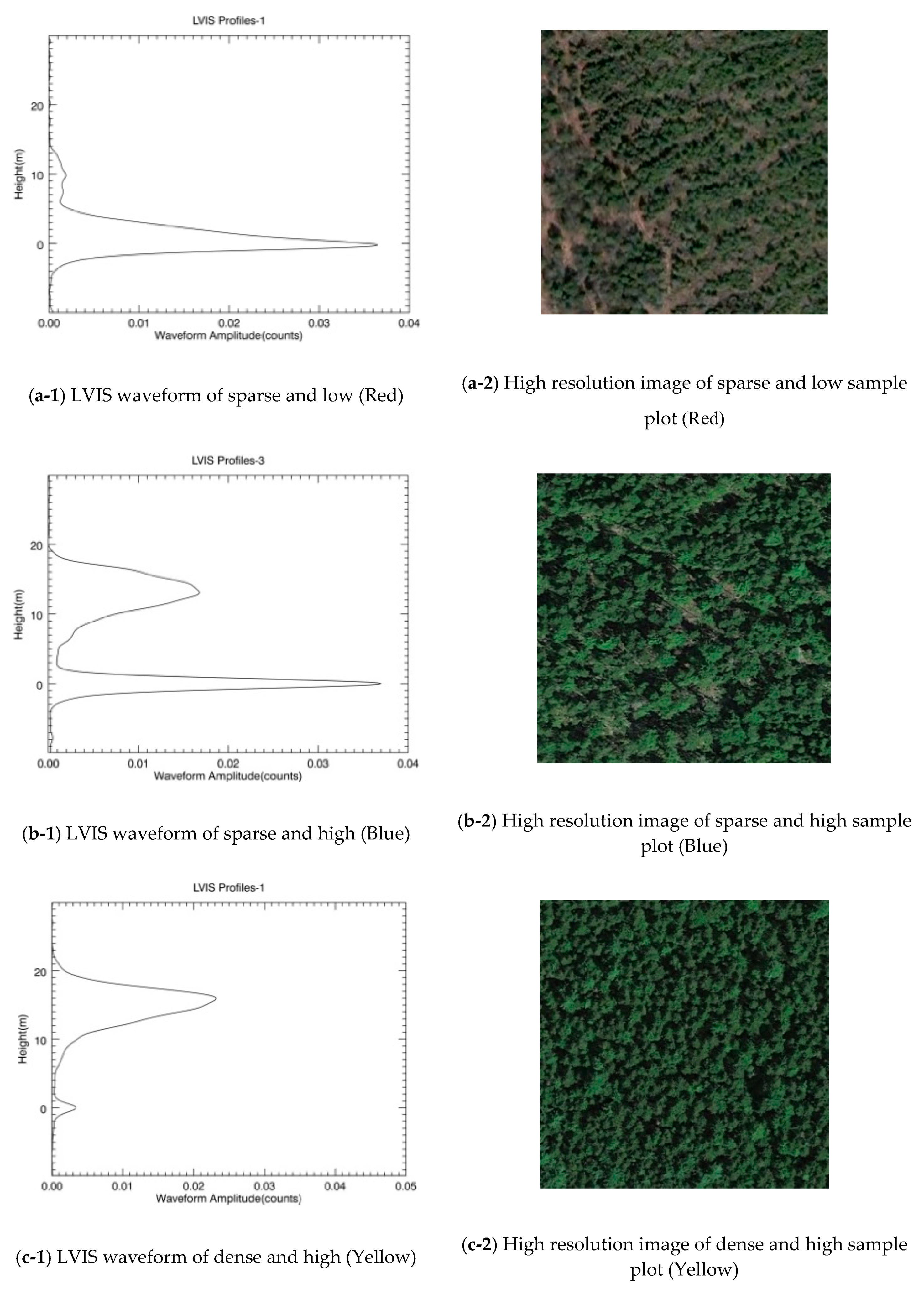
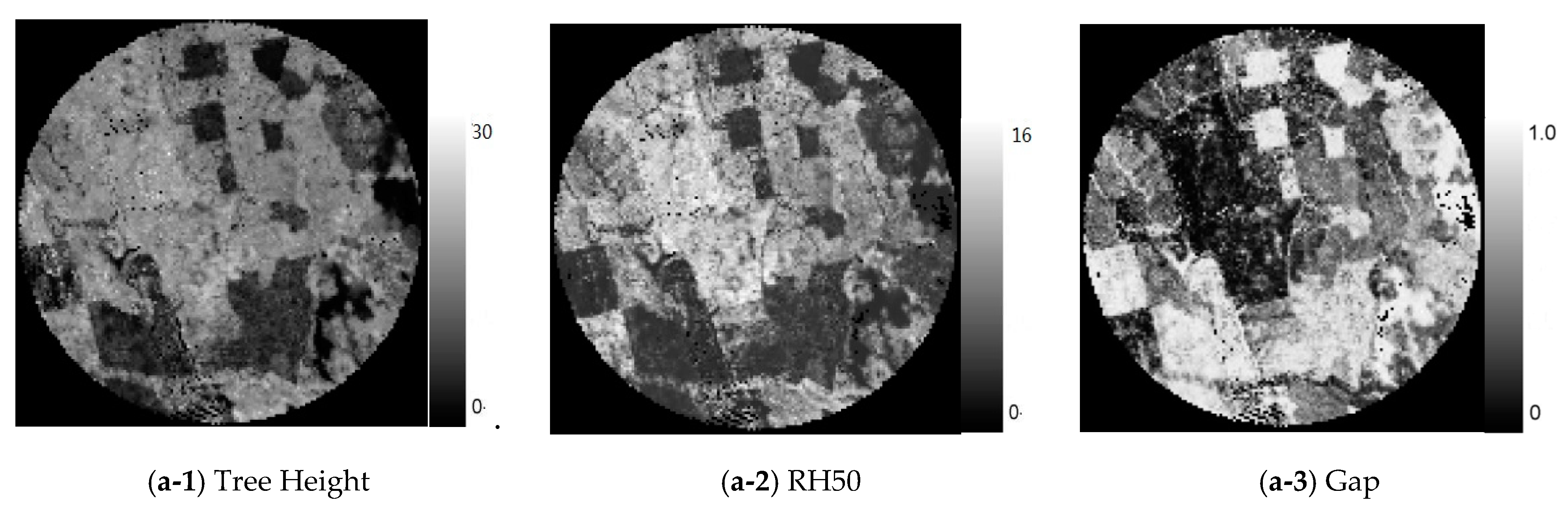
The ratios of the ground’s laser energy returns over the total laser energy returns in Figure 2(b-1), (a-1) gradually increase, and the tree heights in Figure 2(b-1),(a-1) gradually decrease. This occurs because under the same site conditions and the same species, when the tree height is small and the canopy width is relatively small, the gaps between the trees and leaves are relatively high. As the trees grow, although some trees die due to intraspecific competition, these gaps decrease with an increase in the canopy’s horizontal and vertical size. Usually, taller trees or trees with larger crown layers are bigger trees that have smaller gaps between their trees and leaves (without human intervention). However, these gaps are not exactly equivalent to the cover. The gaps are three-dimensional parameters used to describe the gaps from the top to the underside of the canopy between the trees, and between the leaves and twigs within the canopy. Moreover, traditional cover only describes the horizontal structure of the canopy. For small and dense trees, their horizontal cover is high, and their gaps are also relatively high because the layer of a small tree canopy is thin, and most LiDAR pulses can penetrate the canopy and return from the ground to the LiDAR sensor.

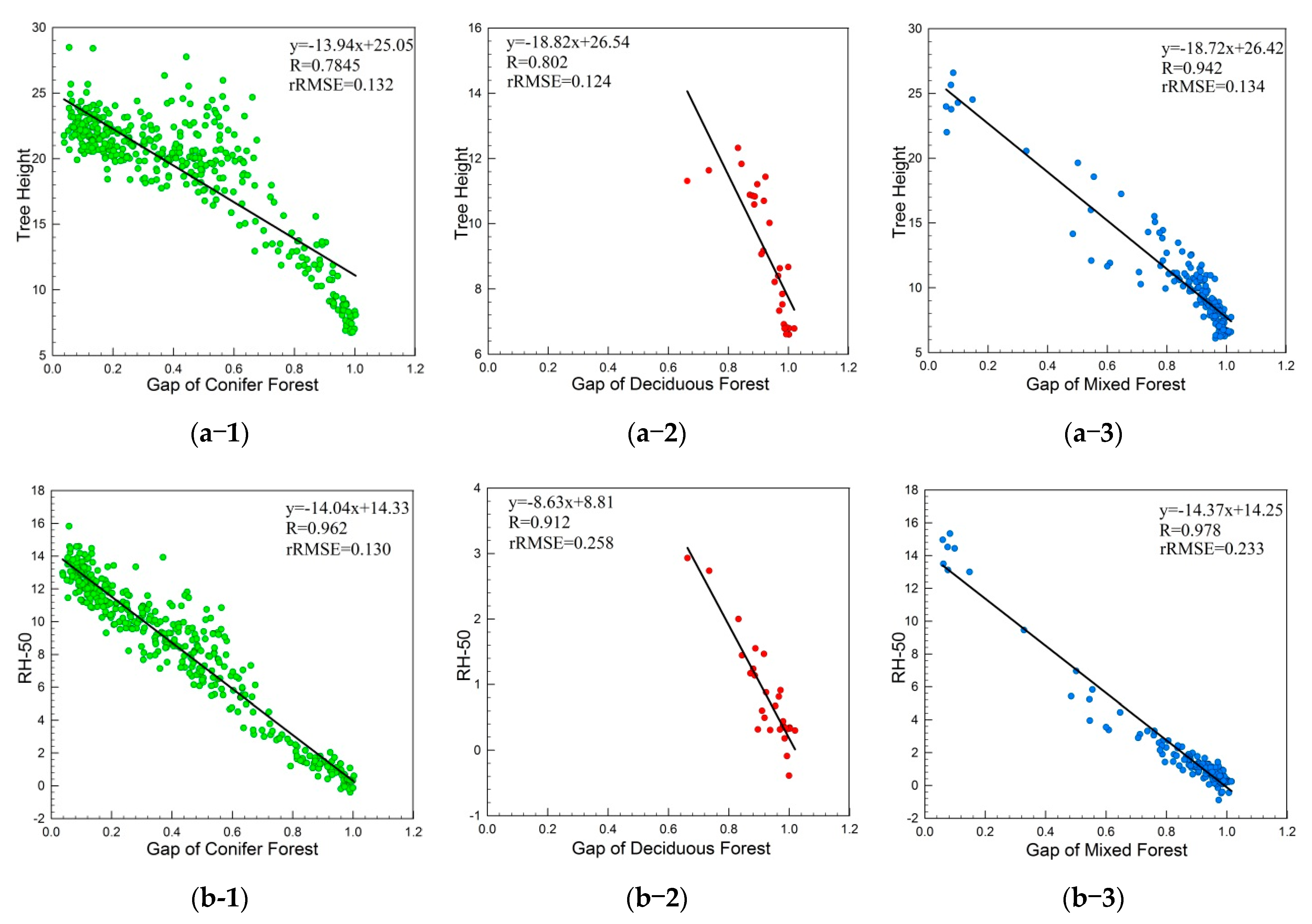
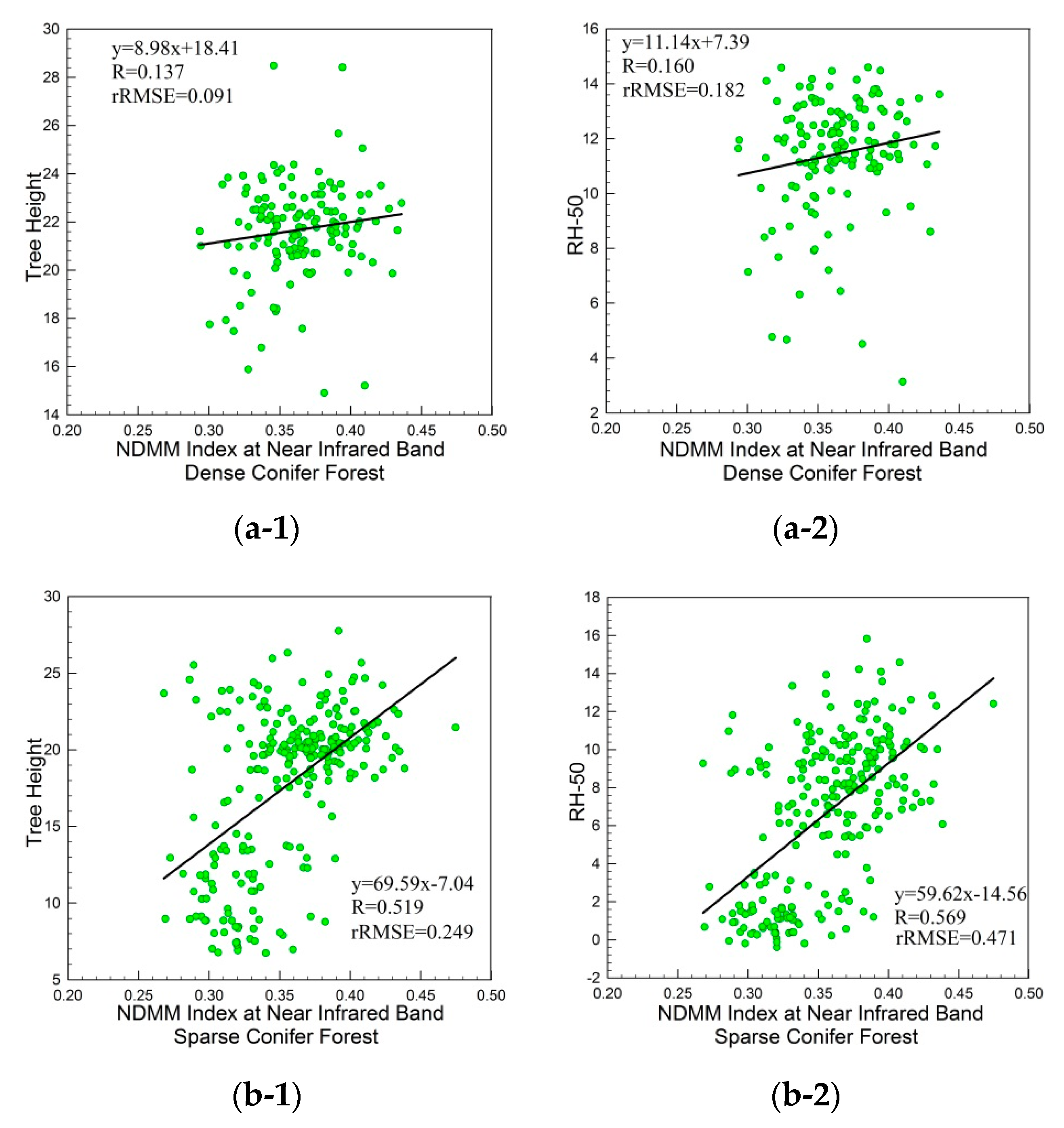
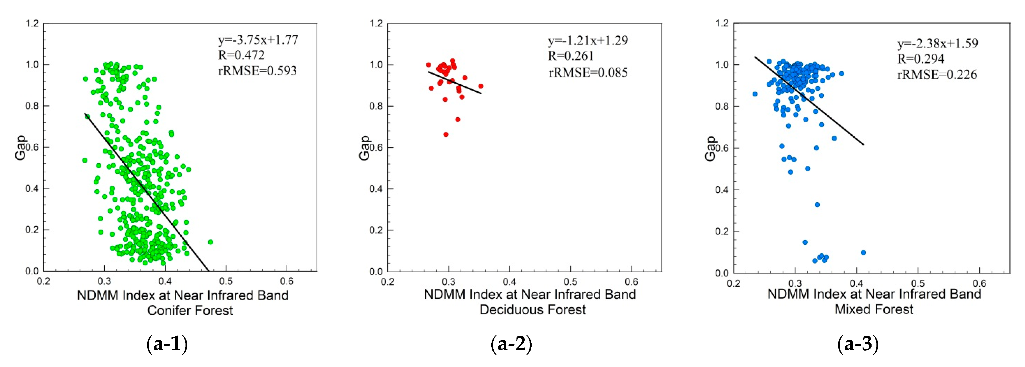
In this paper, three pieces of information were determined from the results. Firstly, Figure 6 and Figure 9 show that the relationships between the LiDAR-derived tree height, gap fraction, and NDMM index depend on tree species because the ratio shape for the four components of BRDF changes due to the shadowing effect of the tree canopy, when the sun and viewing directions change. The conifer canopy’s shape is simple and consistent. Its individual canopy is more prominent than that of the deciduous and mixed forests, and there is a better relationship between the NDMM index and canopy structure, which is mainly sensitive to tree height. 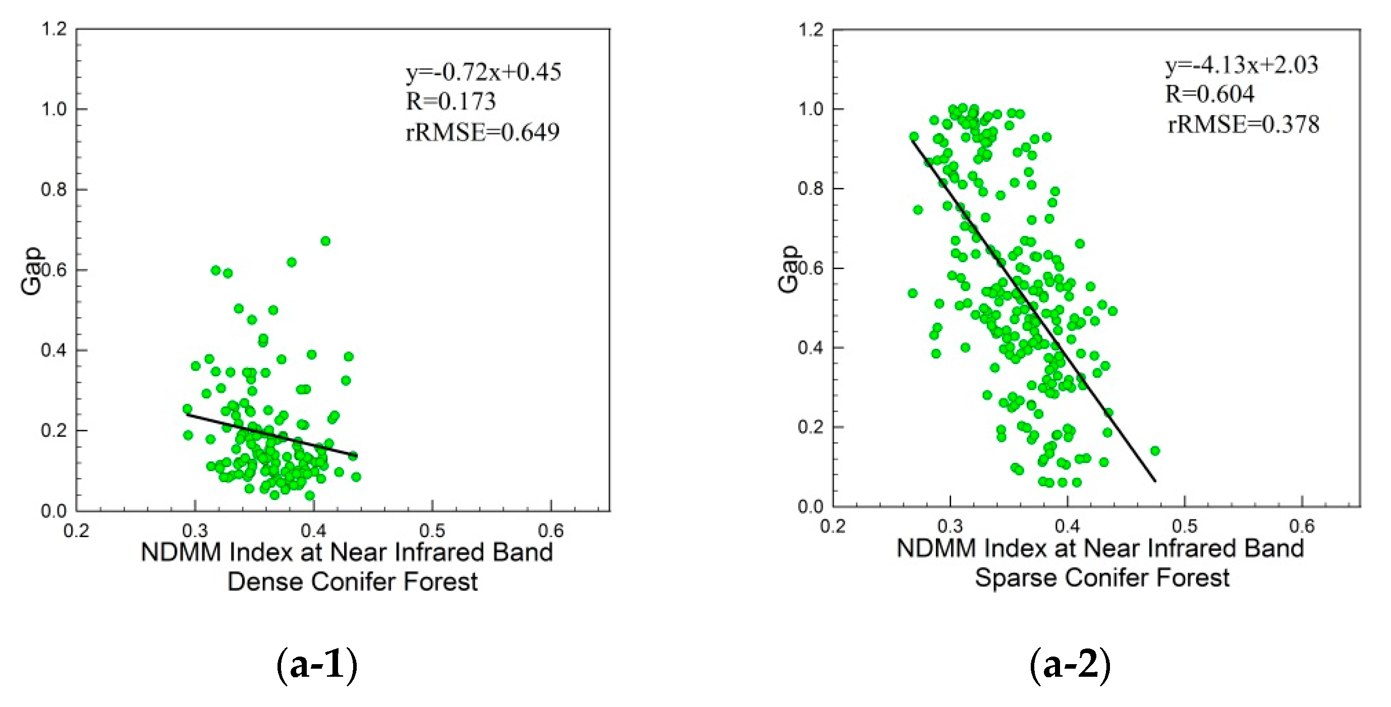Secondly, Figure 7 and Figure 10 show that these relationships also depend on stand density. The higher the tree height and the larger the NDMM index of the canopy, the lower the tree height and the smaller the NDMM index of the canopy. Especially in the sparse and low (Red) and sparse and high (Blue) research areas, a dark color represents a relatively sparse stand in the tree high map. The NDMM indexes for this region are also small in the thematic NDMM index map. That result shows that the Pearson correlation coefficients between the LiDAR-derived tree height and NDMM index for sparse forest is better than that for density. There is a high overlap between the tree canopies in dense forests, such that the individual tree crowns are not prominent, and the four components cannot vary significantly with the sun and view directions changes. The BRDF curve shape does not change significantly with the zenith angle, and even the NDMM index shows a saturation phenomenon. Because of the high density and overlap, there is intense competition within the tree, which results in a decline of the correlation between tree height and canopy structure parameters. The four components that determine the shape of the BRDF curve have a strong correlation with the tree canopy’s size and distribution, which also determines the relationship between the tree canopy’s structural parameters and the NDMM index. While the stand density is low, the individual tree canopy is prominent, and a change in the four components is sensitive to changes of the zenith angles. The correlation between tree height, gap fraction, and the NDMM index in sparse stands is better than that in dense stands.

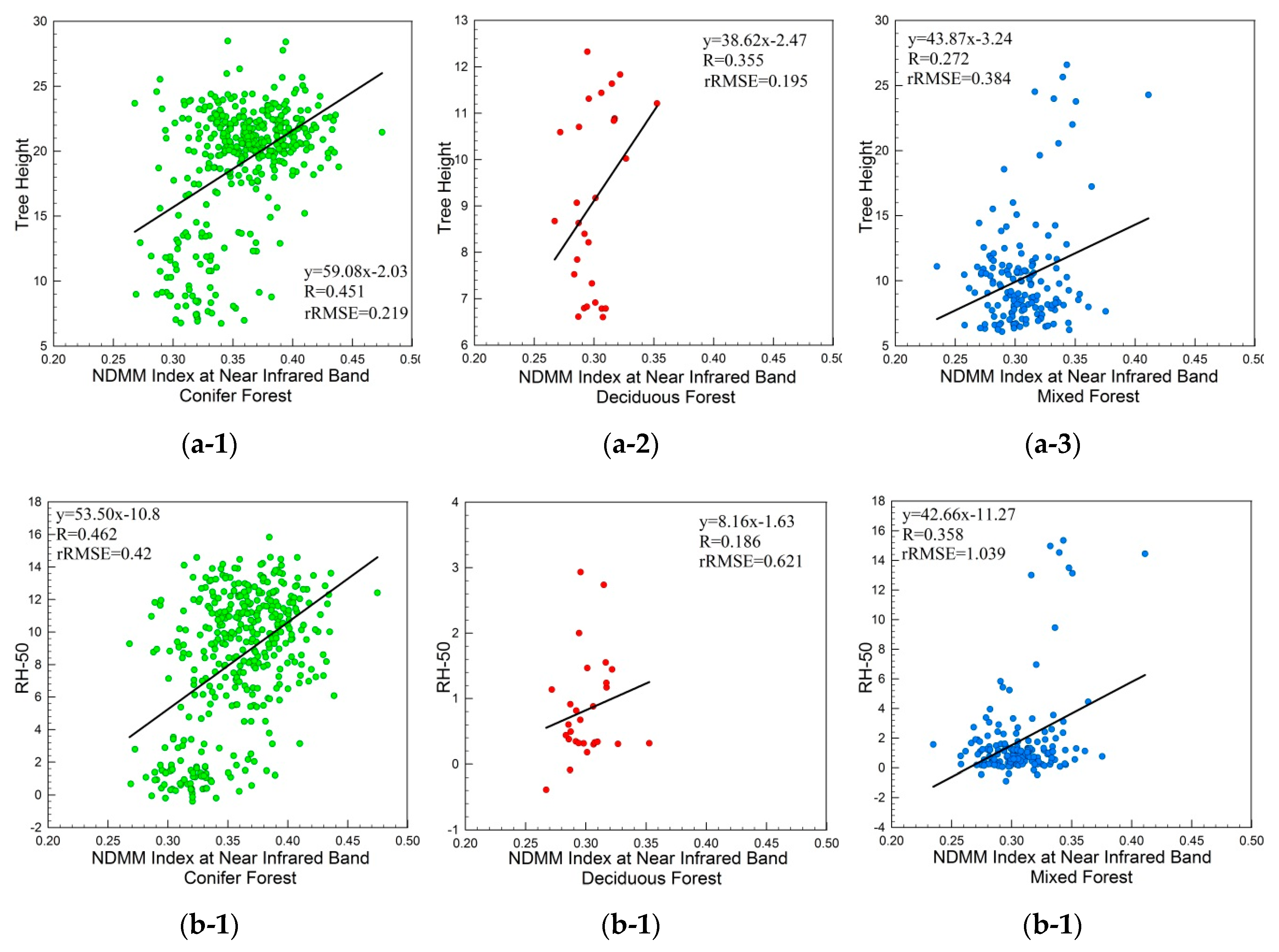
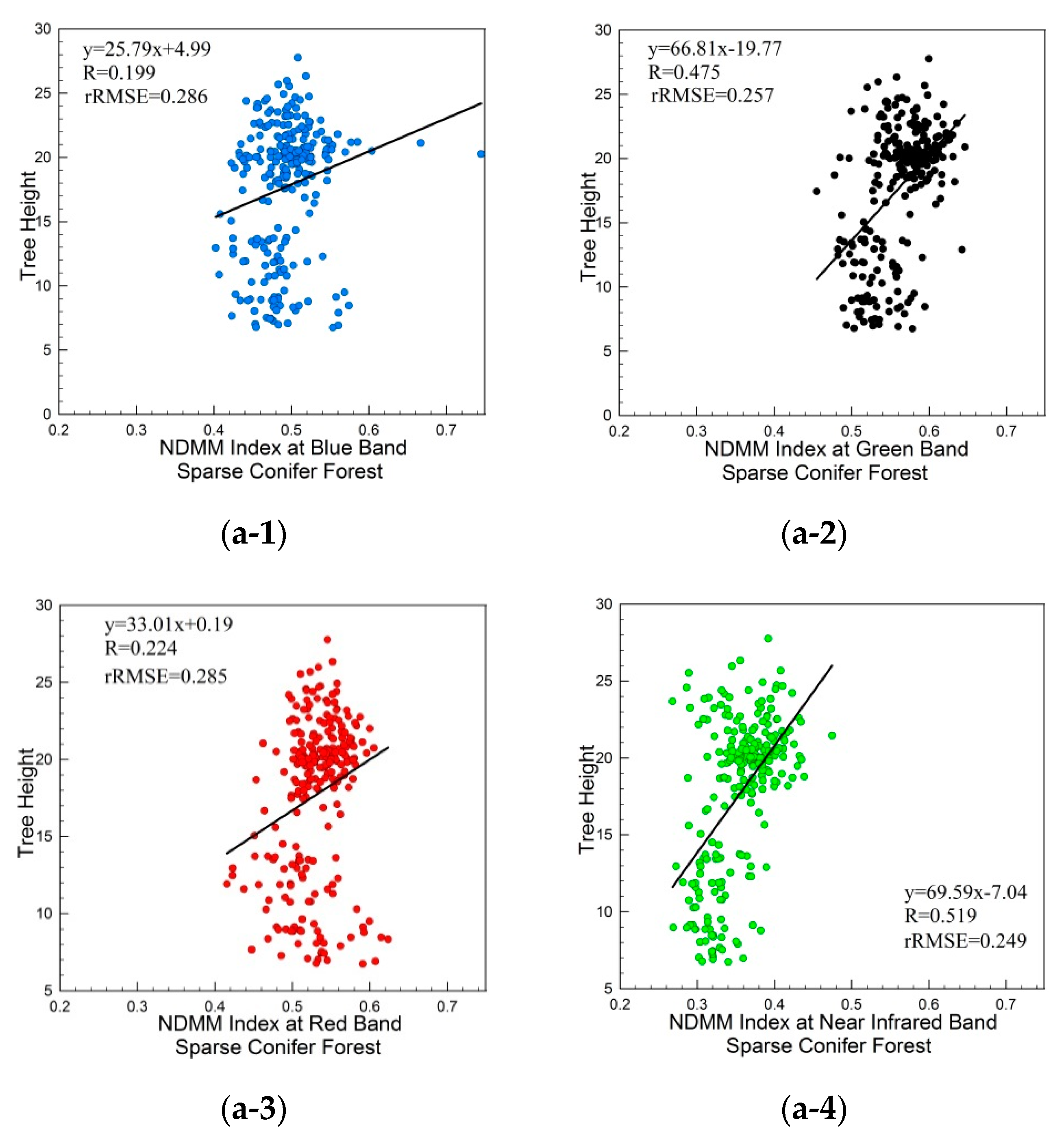
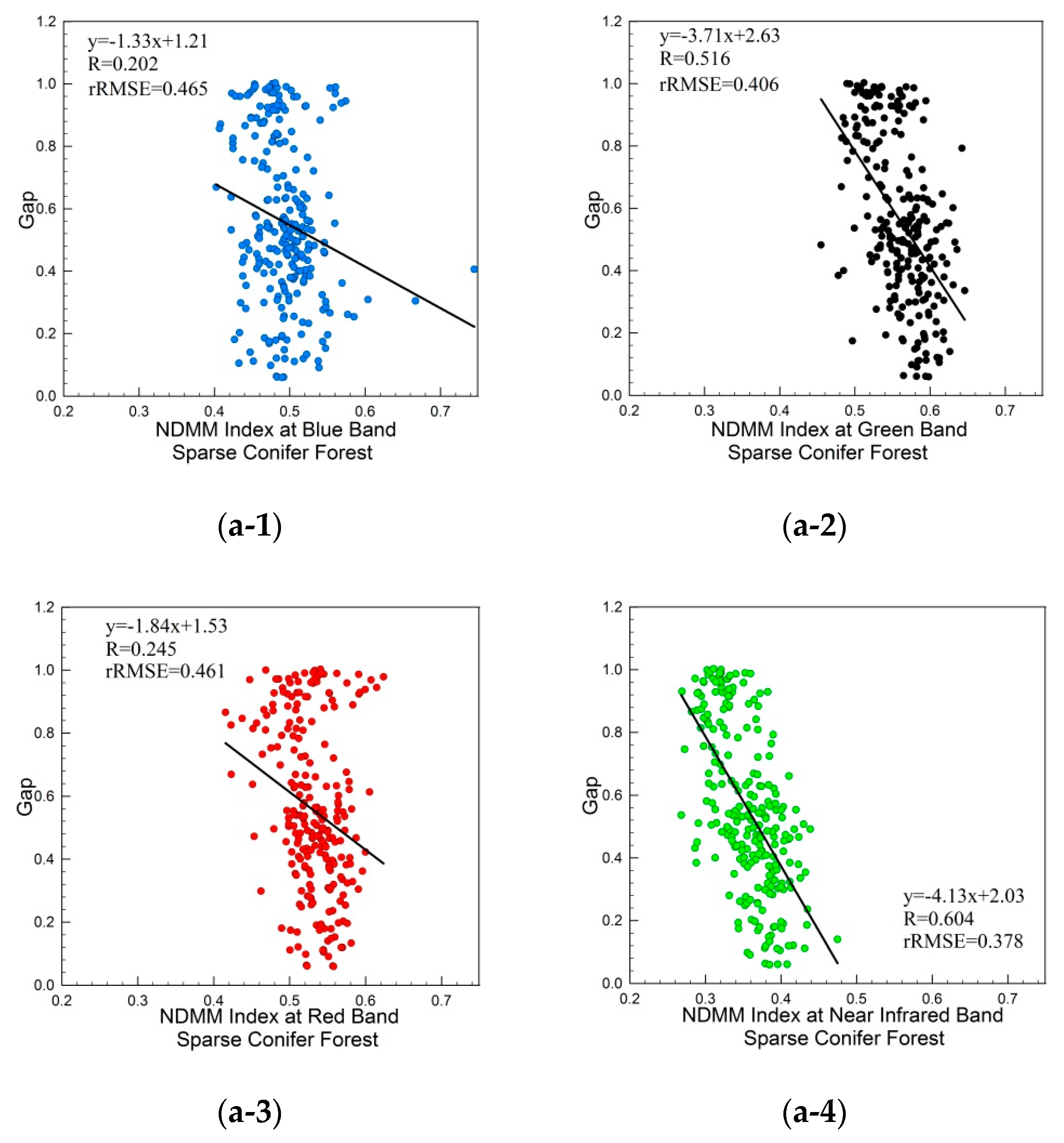
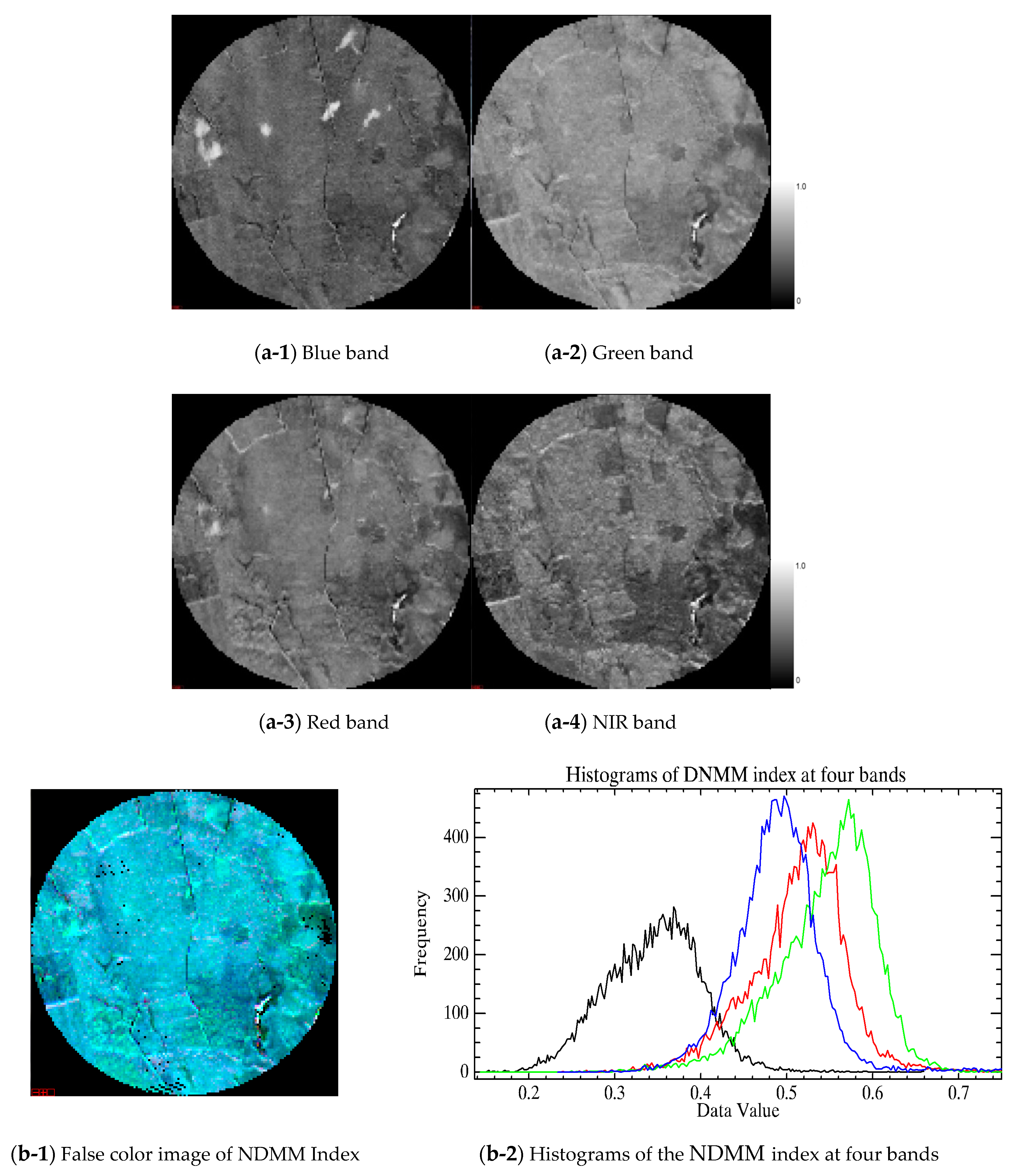
Thirdly, Figure 8 and Figure 11 show that the relationships between LiDAR-derived tree height, gap fraction, and NDMM index are also wavelength dependent. Multiple scattering and shadowing are the main reasons for the differences between the near infrared and visible bands. These effects are due to the higher absorption of the green vegetation of red and green bands, and the reflectance of leaves is high, whereas their transmittance and absorption are low at the near-infrared band because the chlorophyll in leaves can perform photosynthesis under sunlight [32]. The higher single scattering albedo at the near-infrared band leads to more multiple scattering within canopies, among canopies, and between canopies and the background, which results in brighter signatures for all scene components in the near-infrared band than in the blue and red bands. The BRDF value is affected significantly by multi-scatterings between the canopy and backgrounds and among canopies [33,34]. The BRDF curves at the near-infrared band are dependent on the ratio of the four components and have a relationship with the tree structure parameters. However, considering orbital imagery, the visible bands with low reflectance are also strongly influenced by shadowing, and at the blue and red bands, the shadowing reflectance is so weak that the BRDF curves at two bands are not dependent on the ration of the four components, so the BRDF shape is not dependent on the canopy structure, and the NDMM index at the blue and red bands is not sensitive to the tree height and gap faction.

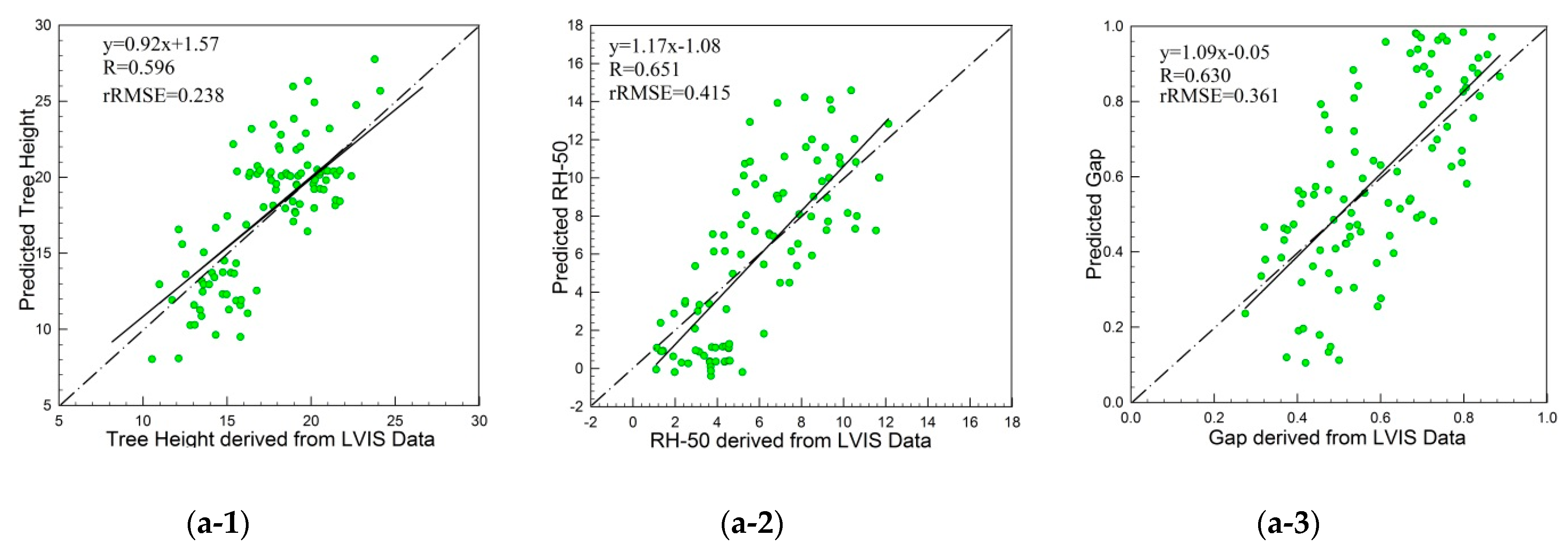
Figure 11 also shows a better relationship between the LiDAR-derived tree height and the NDMM index for sparse conifer forests at the near-infrared wavelength than at other visible optical wavelengths, and the NDMM index linearly increases with tree height. Figure 12 shows the scatterplots for tree height and the gap values derived from LVIS compared to those predicted by the NDMM index at the near-infrared band for sparse confer forests in Howland. In Figure 12, the dotted line is the 1:1 line, and the solid lines are the scatterplots for the tree height and the gap values derived from LVIS versus those predicted by the NDMM index at the near-infrared band for sparse confer forests in Howland. The LiDAR-derived tree height, gap, and the values predicted by the NDMM index are near the 1:1 line, which indicates that relationships between tree height and gap values are inverted by the NDMM index and LiDAR-derived tree height. The gap values are consistent with the results in Figure 7(b-1),(b-2) and Figure 11(a-4). It is known that the BRDF exhibits a half-bowl shape with a peak value in hotspots. That is, when the sun and viewing directions are the same, the higher the tree is and the larger the canopy volume and surface area are, so individual trees are more prominent. There is an increase in the observed sunlit crown components and the relatively bigger canopy; the sunlit crown component is larger than the sunlit background component, which contributes more to the whole BRDF shape. The maximum reflectance value is higher according to the largest area proportion of the sunlit crown component, because the bigger canopy volume and surface area cause the sunlit and shaded crown components to be larger, and the difference between the sunlit and shaded crown components is also larger. The BRDF shows an unsymmetrical shape, with its minimum at an angle in the forward direction (sun and satellite in opposite directions) and its maximum in the backward direction (sun and satellite at the same direction). The differences of the maximum directional reflectance in the forward direction and the minimum directional reflectance in the backward direction are larger and cause the NDMM index to be bigger. On the other hand, with a shorter tree and smaller canopy volume and surface area, there is a decrease in the sunlit crown components observed and a relatively smaller canopy. The difference between sunlit and shaded crown components decreased, so the difference of the maximum directional reflectance in the forward direction and the minimum directional reflectance in the backward direction also decreased and caused the NDMM index to become smaller. As shown in Figure 7(b-2), when the BRDF value is lower (between 0.25 and 0.35), the height, size, and density of the tree canopy are smaller. However, most of the laser energy transmits through the tree canopy and reaches the background, and the echo energy of the background makes up a large proportion of all the laser echo energy in the footprint, and the RH50 value is less than zero.

Our analysis demonstrates that the NDMM index from visible to near infrared wavelengths increases according to LiDAR-derived tree height and RH50 and decreases with a gap fraction in all three types of forests: conifer, deciduous, and mixed. The BRDF’s shape is directly controlled by the brightness and areal proportions of the sunlit and shaded canopy and background. As the viewing angle changes, these four components are directly related to canopy height and variation, crown size, density, and the spectral properties of the leaves and the background, according to the Geometric Optical-Radiative Transfer (GORT) model. The NDMM index describes the changes in BRDF due to viewing angle differences and is directly linked to vegetation-structure parameters. This study demonstrates a reasonable relationship between BRDF measurements with tree height and the gap fraction derived from LiDAR in sparse conifer forests. However, the multiangular NDMM index used the bidirectional reflection signal of the tree canopy to invert the forest-structure parameters. Moreover, a tree’s canopy is considered to be one of the most important factors that affect the tree’s growth, because a tree canopy intercepts 80% of solar radiation and is the main site of a series of physiological activities, such as photosynthesis, respiration, and transpiration. The size, structure, shape, and spatial distribution of a canopy can directly determine growth vigor, productivity, and overall tree growth. Further, the canopy is one of the main components of individual tree biomass. In particular, the two paramount directional signals, the maximum and minimum angle reflectance, contain the greatest amount of forest canopy information, which is indirectly linked to other forest-structure parameters, such as tree height, forest density, leaf area index (LAI), and even the forest’s biomass.

6. Conclusions

This was an exploratory study to investigate how a single anisotropic index calculated from multiangular measurements is related to the LiDAR-derived vertical structure parameters of vegetation. Based on the result, the physics of the relationships between the multiangular signal and forest canopy structure parameters were studied and assessed using airborne LiDAR data, and multiangular remote sensing data were used to map the forest parameters at larger regions with more complete geographic coverage. We found better relationships between the LiDAR-derived tree height, gap fraction, and NDMM index at the near-infrared band for sparse conifer forests in Howland. The difference between maximum and minimum reflectance from different angles includes the main three-dimensional structural information of a forest canopy. This paper presented a new and potential NDMM index to retrieve the tree heights and gap fractions from multiangular data.

However, for the relationships between the NDMM index and LiDAR-derived tree height, the gap also varies according to tree species, stand density, and wavelength. As the Pearson correlation coefficient between the NDMM index and tree height, the gap fraction shows that the NDMM index for conifer forests is better than those of deciduous and mixed forests. For the relationship between the NDMM index and LiDAR-derived tree height, gap fraction also varies with stand density, and the conifer forest is superior to the dense forest. The results show that the NDMM index at the near-infrared band is better than three other visible bands. Gao, et al. [24] also showed that an evergreen needle leaf forest has a more constant geometric effect than that of deciduous and mixed forests, and the relationship at blue and red wavelengths is weak, which is consistent with the results of previous studies by Kimes, et al., which show that the relationship at the near infrared wavelength is better.

The BRDF vegetation structure retrieval works better in conifer forests, which indicates that forest biomass retrieval based on the NDMM index can be used to understand how to take advantage of the implied information between multiangular data and forest canopies. In this respect, the feasibility of retrieving the structural properties of a tree canopy from different satellite observations is a challenge. This challenge will provide scientific evidence for more rigorous models. Further studies using GORT models are needed to better understand the physics of the relationships between the NDMM index and the forest canopy’s structural information observed in real airborne LiDAR and AirMISR data. Starting with this paper, better anisotropic factors will be developed to link LiDAR-derived vegetation-structure parameters and multiangular remote sensing data to map vegetation structure parameters at larger regions for carbon cycle studies.