Article

Covariance Analysis of Real-Time Precise GPS Orbit Estimated from Double-Differenced Carrier Phase Observations

1
School of Mechanical and Aerospace Engineering and SNU-IAMD, Seoul National University, Seoul 08826, Korea
2
Ecole Nationale de l’Aviation Civile (ENAC), 31400 Toulouse, France
*
Author to whom correspondence should be addressed.
Remote Sens. 2019, 11(19), 2271; https://doi.org/10.3390/rs11192271
Submission received: 23 August 2019 / Revised: 25 September 2019 / Accepted: 26 September 2019 / Published: 28 September 2019

Abstract

:
The covariance of real-time global positioning system (GPS) orbits has been drawing attention in various fields such as user integrity, navigation performance improvement, and fault detection. The international global navigation satellite system (GNSS) service (IGS) provides real-time orbit standard deviations without correlations between the axes. However, without correlation information, the provided covariance cannot assure the performance of the orbit product, which would, in turn, causes significant problems in fault detection and user integrity. Therefore, we studied real-time GPS orbit covariance characteristics along various coordinates to effectively provide conservative covariance. To this end, the covariance and precise orbits are estimated by means of an extended Kalman filter using double-differenced carrier phase observations of 61 IGS reference stations. Furthermore, we propose a new method for providing covariance to minimize loss of correlation. The method adopted by the IGS, which neglects correlation, requires 4.5 times the size of the covariance to bind orbit errors. By comparison, our proposed method reduces this size from 4.5 to 1.3 using only one additional parameter. In conclusion, the proposed method effectively provides covariance to users.

Graphical Abstract

1. Introduction

In recent years, precise real-time global positioning system (GPS) orbit products have extended the capability to support real-time applications such as autonomous driving, intelligent transportation systems, and collision avoidance [1,2]. The real-time precision of orbits enables navigation systems to overcome problems arising from orbit errors in real-time observations [3].
Precise real-time GPS orbits have been determined with the international global navigation satellite system (GNSS) service (IGS) forming the mainstream service. IGS provides ultra-rapid orbits as real-time precise orbits [4]. Ultra-rapid orbits are determined using recent satellite arcs of 3 days to predict the orbit for 24 h thereafter [5]. The maximum accuracy of the predicted orbit is 5 cm at 1D root mean square (RMS). Another such service is the IGS real-time service, which is supported by ten analysis centers [2]. One of the analysis centers, the Centre National d’Études Spatiales (CNES), estimates the satellite orbit and clock together using undifferenced GPS observations. Other IGS analysis centers often use ultra-rapid solutions for precise orbits and concentrate on precisely estimating satellite clocks [6,7,8]. Furthermore, precise point positioning (PPP)-based commercial services have similar strategies to generate precise orbits and clocks when compared with IGS real-time products. Past studies have focused on verifying the accuracy of these real-time precise orbits [5,8,9].
Interest in the covariance of real-time precise GPS orbits, as well as in the accuracy, has increased in the context of user integrity, navigation performance improvement, and fault detection [10,11,12,13]. In terms of safety, covariance is one of the most important factors that provide integrity that ensures correct position information. Range error due to orbit error should be overbounded to ensure user position integrity [14,15]. In general, systems provide the accuracy of signal-in-space range error (SISRE) or orbit full covariance. The accuracy of SISRE is calculated with proper weightings for radial, along-track, and cross-track standard deviations [16,17]. Providing full covariance enables each user to propagate the accuracy of SISRE by projecting the error ellipsoid along its line of sight [11], which can reduce specific accuracy of SISRE according to the various positions of the users [12]. Therefore, to generate appropriate accuracy of SISRE, proper error ellipsoid which contains the true orbit should be obtained.
However, orbit full covariance is not provided from real-time orbit products. Previous studies utilized the maximum accuracy or the stochastics of orbit errors to analyze the effect of covariance usage. El-Mowafy suggested using the orbit covariance to detect faults or meaconing errors in IGS RTS correction and demonstrated the significant advantage of a new fault detection model over traditional models under a meaconing attack [18]; the expected effect of covariance was considered using the maximum accuracy of each axis, which is greater than the full covariance. The full covariance would provide orbit uncertainty more appropriately and would improve the performance of fault detection. In addition, Cheng et al. [19] analyzed the user range accuracy performance of real-time ephemeris. They studied the characteristics of long-term error stochastics over a year to provide the performance of user range accuracy. However, as only the average characteristics can be obtained over a long duration, the correlation for real-time covariance should be analyzed for real-time applications. Therefore, we estimated the real-time orbit covariance to identify more realistic covariance characteristics.
To support covariance-based applications, IGS plans to provide real-time full covariance, although it is not expected to be provided shortly in the near future [20]. The real-time orbit standard deviation is presently provided over the XYZ components of the Earth-centered Earth-fixed (ECEF) frame, without any correlations between the axes. However, if the correlation information is neglected, the provided accuracy cannot ensure the performance of the orbit product, which in turn causes significant problems in fault detection and user integrity. Therefore, it is safe to provide a conservative representation of the orbit error distribution, however unnecessary overbounding decreases the availability of the system.
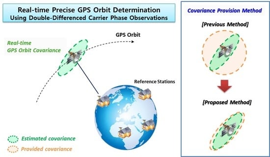
This paper proposes an effective covariance provision method considering the correlations of real-time GPS orbits. We analyzed these correlations using a real-time GPS precise orbit estimator and studied the covariance along various coordinates. The results demonstrate the real-time characteristics of the correlations, which cannot be determined based on long-term analyses. Considering the correlation, we propose a covariance provision method and evaluate it using the number of parameters and ratio of the provided covariance volume to the full covariance volume.
The remainder of this paper is organized as follows. Section 2 presents the details of the orbit determination tool and the theoretic background of real time orbit covariance due to orbit dynamics; Section 3 discusses the experimental results; Section 3.1 verifies the orbit determination system in relation to the IGS final orbit; Section 3.2 presents the experimental results of covariance analysis and proposes a new frame to minimize correlations between the axes; Section 3.3 assesses several covariance provision methods; Section 4 discusses our findings; and finally, Section 5 presents our conclusions.

2. Orbit Determination Filter Algorithm

2.1. Observational Data

This study uses double-differenced carrier phase (DDCP) to focus on orbit determination without clock errors. To obtain cm-level accuracy, CP observations are generally used to determine precise orbits. CP is defined as the phase difference between the satellite and the receiver, and it contains satellite clock errors and receiver clock errors in addition to the distance information between the satellite and receiver [21]. Additionally, there are phase center offsets (PCO) and variations (PCV), phase wind up (PWU) and tidal effects, which are generally corrected by models for GPS precise orbit determination [22]. Researchers normally use these observations in the form of un-differenced CP (UDCP) or DDCP data. Clock errors can be eliminated by means of the double-differencing method. Furthermore, if the network comprises the same type of receiver, the hardware bias is also eliminated with the double-differencing method. In contrast, the noise of the receiver is doubled. Table 1 compares the error components of UDCP and DDCP, wherein ‘V’ indicates the presence of an error component.
The DDCP L1 and L2 terms can be expressed as follows:
Δ φ L 1 = Δ d + Δ T Δ I L 1 + Δ N L 1 λ L 1 + Δ ε Δ φ L 1
Δ φ L 2 = Δ d + Δ T f L 1 2 f L 2 2 Δ I L 1 + Δ N L 2 λ L 2 + Δ ε Δ φ L 2
where Δ denotes the double difference operator; φ the CP observation; subscripts L1 and L2 the L1 and L2 frequencies, respectively; d , T , and I the distance, tropospheric delay, and ionospheric delay, respectively; f the frequency; N an integer ambiguity; λ the wavelength; and ε the measurement noise.
Furthermore, this study uses the Melbourne–Wübbena (MW) combination to resolve the wide lane (WL) integer ambiguity, and subsequently, the WL ambiguity is applied to the ionosphere-free (IF) combination to guarantee the integer nature of the observation ambiguities. The MW is defined as the difference of the WL combination CP and the narrow lane (NL) combination pseudo-range (PR). The DDCP MW and DDCP IF can be expressed, respectively, as follows [23]:
Δ φ M W = Δ φ W L Δ ρ N L Δ N W L λ W L + M Δ φ M W + ε Δ φ M W
Δ φ I F = f L 1 2 f L 1 2 f L 2 2 Δ φ L 1 f L 2 2 f L 1 2 f L 2 2 Δ φ L 2 = Δ d + Δ T + Δ N f l o a t + ε Δ φ I F
Δ N f l o a t = f L 1 2 f L 1 2 f L 2 2 Δ N L 1 λ L 1 f L 2 2 f L 1 2 f L 2 2 Δ N L 2 λ L 2 = Δ d + Δ T + Δ N f l o a t + ε Δ φ I F
where M denotes the multipath error, ρ the PR, and Δ N f l o a t a float ambiguity in the DDCPIF observation. Thus, the orbit filter estimates the tropo wet zenith delay and L2 integer ambiguity as well as satellites’ position and velocity.

2.2. Filter Architecture and Details

The architecture of the real-time precise GPS orbit filter is shown in Figure 1. The inputs to the filter are raw measurements, the broadcast (BRDC) orbit, and the International Earth Rotation and Reference System (IERS)-predicted earth orientation parameters (EOP). Raw measurements are acquired in the RINEX format from the IGS data archive [22]. Dual-frequency PR and CP data are acquired from 61 globally distributed stations across 30 s intervals. Figure 2 shows the station locations and baselines. The stations are chosen to form a station network with homogeneous receivers, Trimble receiver in this case, in order to avoid estimation of hardware bias errors. The mask angle is set to 5°. The IERS-predicted EOP is used for coordination transformation, and broadcast ephemeris is used for preprocessing.
First, the raw data are preprocessed to detect and compensate for cycle slips. Subsequently, the main filter uses the ‘cleaned’ CP to determine the orbit and its covariance. The main filter state consists of the satellite position, vector, coefficients of solar radiation pressure, wet zenith tropospheric delays, and ambiguities. For more accurate orbit results, the main filter should resolve the L2 ambiguities. In this step, the fixed WL ambiguity is required. Therefore, the WL ambiguity filter estimates the WL ambiguity using DDCPMW observations beforehand. To mitigate the effect of multipath, this filter also estimates the multipath error as well as WL ambiguity by modeling the first-order Gauss-Markov process [24,25]. The detailed method is described in [24]. Finally, the GPS orbits and their covariance are generated in real-time. Table 2 and Table 3 show the states of the WL ambiguity filter and main Kalman filter.

2.2.1. Preprocessing

In order to generate precise orbits, the cycle slip should be detected and compensated. Cycle slip is a discontinuity that appears when a receiver experiences a loss of lock [21]. This study adopted the preprocessing algorithm proposed in the Bernese GNSS software [26]. First, a DDIF observation was fitted with the second-order polynomial for outlier and cycle slips. Second, the time-differenced MW and ionosphere combinations were utilized to detect and compensate for the cycle slip. The algorithm was verified in reference [24].
Several additional corrections are considered in this preprocessing step. When the baseline length is small, errors such as phase wind up and tidal displacements can be eliminated with the double differencing method [3,27]. However, the baselines of our network, which range from 120 to 3800 km, are too long to neglect the extra errors. Therefore, we compensated the errors; Table 4 summarizes the corresponding strategy [28,29,30,31]. The strategies use the GPS attitude model for nominal attitude [28], which is also called yaw-steering attitude.

2.2.2. Main Filter Description

The main filter utilizes a sequential extended Kalman filter (EKF) for real-time orbit determination. The sequential approach processes incoming data immediately, and can quickly respond to and reflect the real-time orbit [32]. The EKF utilizes two steps: time update (TU) and measurement update (MU) steps. The orbit and covariance are estimated over repeated TU and MU iterations. The orbit is initialized with the broadcast orbit, and the initial standard deviation is set to 2 m for each axis.
In the TU step, the previous step state is propagated with system dynamics. The state of the satellite position and velocity are propagated by orbit dynamics. On the other hand, the troposphere wet zenith delay of every station makes use of the first-order Gauss–Markov process as the propagation model. The coefficients of solar radiation pressure and L2 integer ambiguities are estimated together. The state transition matrix of the orbit position and velocity requires numerical derivatives. The setting values of filter is described in Table 5 and Table 6.
The MU step is performed using the DDCPIF observations of the network. To estimate the troposphere wet zenith delay, we eliminate the dry component using the Saastamoinen model [33]. Furthermore, the dry and wet mapping function is based on the Niell mapping function [34].

2.2.3. Orbit Propagation

Each satellite orbit is propagated by means of the Runge–Kutta 68 numerical integral method [32] using satellite dynamics. The integration step is 30 s. For the orbit propagation, the state and dynamics utilize the J2000 coordinate system. The equinox-based transformation is implemented using IAU-2000A as per [35]. The satellite acceleration is calculated with the use of Cowell’s method [36], which adds perturbing accelerations to the two-body equation to generate a more accurate equation of motion. The satellite acceleration is expressed, as follows:
a = μ | r | 3 r + a G e o p o t e n t i a l + a T h i r d - b o d y + a S o l a r   r a d i a t i o n   p r e s s u r e + a T i d e + a G e n e r a l   r e l a t i v i s t i c
where r and a the position and acceleration, respectively.
We add the perturbing effects of the non-spherical central body, the third-body effects of the Sun and Moon, solar radiation pressure, and the tides. The Earth’s gravitation field is implemented as per the earth gravity model (EGM) 96 and is truncated to the 12th degree and order for GPS orbits [37]. Third-body effects consider the Sun and Moon as the third planet, and utilizes the DE405 planet model [38]. Tidal and general relativistic effects are examined following IERS 2010 standards. For solar radiation pressure, precise GPS orbit products estimate the coefficients of the model of dynamics in general. The Empirical Center for Orbit Determination in the Europe Orbit Model (ECOM) [39] is a popular dynamics model for real-time GPS orbit products [40,41]. We applied the ECOM model with nine radiation pressure terms for each satellite. The nine coefficients per satellite are estimated together. In addition, the shadows of the Earth and Moon comprise a conical model [42]. Table 7 summarizes the dynamic model.

2.3. Propagation Characteristics of Orbit Dynamics

Before the experimental analysis, we briefly explain the characteristics of covariance theoretically by means of orbit dynamics. In general, the orbit error can be induced as the relative movements of two objects, where one orbit is on the true orbit and the other is on the estimated orbit. The orbit propagation properties have been studied using relative motion equations in the RSW frame [43,44,45].
The geometric modeling of relative motion can express orbit error by means of orbital elements as follows for a near-circular orbit [45]:
x δ a acos ( f ) δ e
y 2 asin ( f ) δ e + a ( δ w + cos ( i ) δ Ω + δ M )
z a ( sin ( u ) δ i cos ( u ) sin ( i ) δ Ω )
v x ansin ( f ) δ e an ( δ w + cos ( i ) δ Ω + δ M )
v y n 2 δ a + ancos ( f ) δ e
v z an ( cos ( u ) δ i + sin ( u ) sin ( i ) δ Ω )
where, x , y , z , v x , v y , and v z represent the orbit errors corresponding to the position and velocity vector for each axis in the RSW frame; a ,   e ,   i ,   Ω , w , f and M denote the orbital elements of the semi-major axis, eccentricity, inclination angle, right ascension of the ascending node, argument of perigee, argument of latitude, true anomaly, and mean anomaly, respectively; n denotes the mean motion; and δ is the error of each component.
The semi-major axis error δ a is affected by disturbances, and it is generally modeled by a linear function of time.
δ a = δ a 0 + δ a ˙ τ
It affects mean anomaly M , which is expressed as:
δ M = δ M 0 + δ n τ = δ M 0 3 n 2 a ( δ a 0 τ + 1 2 δ a ˙ τ 2 )
Upon utilizing a linear function of, δ a , x , y , z , v x , and v y can be, respectively, expressed as:
  x δ a τ ˙ acos ( f ) δ e + δ a 0
y ( 3 4 n δ a ˙ τ 2 3 2 n δ a 0 τ ) + 2 asin ( f ) δ e + a ( δ w + cos ( i ) δ Ω + δ M 0 )
v x ( 3 4 n 2 δ a ˙ τ 2 + 3 2 n 2 δ a 0 τ ) ansin ( f ) δ e an ( δ w + cos ( i ) δ Ω + δ M 0 )
v y n 2 δ a ˙ τ n 2 δ a 0 + ancos ( f ) δ e
where τ denotes the elapsed time with propagation, and subscript 0 indicates the initial value; furthermore, δ a ˙ denotes the rate of the semi-major axis error.
Equations can aid us in understanding the orbit propagation characteristics. Errors along the radial and along-track directions consist of secular, periodic, and constant components. The square of parameter τ diverges rapidly as time elapses, and this leads to large variance of the along-track errors. The periodic terms are due to δ e and their period is the same as the orbit period. In general, δ e ,   δ i ,   δ Ω , and δ w are all extremely small.
In addition, the correlation between the radial and along-track values can be explained using Equation (19). The secular component of the along-track error exhibits a proportional relationship with the radial velocity error, and the proportional constant has a negative value and is expressed as:
v x y n
This leads to negative correlation of the errors of the radial and along-track directions. The cross-track position and velocity errors are periodic for the argument of latitude u .

3. Verification of Orbit Filter and Covariance Analysis

First, we present our evaluation of the position results in relation to the IGS final orbits (Section 3.1). Section 3.2 presents the error covariance characteristics over time and for several frames; IGS final orbits are not used. Furthermore, the error correlations between the axes are analyzed. In Section 3.3, these characteristics are utilized to propose and evaluate a new covariance parameterizing method.

3.1. Orbit Filter Results

3.1.1. Experimental Environment

We obtained the results of the orbit filter using the dual-frequency PR and CP of the 61 IGS stations shown in Figure 2; these were collected on 15–16 January 2018. The filter generated real-time orbits at intervals of 30 s. In this section, we present our verification of the filter performance in relation to the IGS final product. The accuracy of IGS final orbit products [46], which are the most precise GPS orbits, is 2.5 cm [47]. The position error is the difference between the estimated satellite positions and the IGS final product. In addition, a simulation was conducted to verify the filter. The simulation data are summarized in Table 8.

3.1.2. Position Errors

Figure 3 shows the time history of the pseudo-random noise (PRN) 9 orbit error of simulation and real data. The red, green, and blue curves denote the 3D position error, radial error, and estimated standard deviation of the 3D position error, respectively. The initial orbit conditions are calculated using the BRDC orbits, and therefore they exhibit meter-level accuracy. The orbit accuracy convergences to the centimeter level after 24 h.
Figure 4 shows the root mean square (RMS) orbit errors of all satellites during the last 24 h of a given day. The mean 3D RMS value is 7.8 cm, and the radial track error is ~2 cm. The along-track error was larger than radial and cross-track errors.

3.1.3. Actual Error Distribution of Real-Time Precise Orbit

We analyzed the actual error distribution of real-time precise orbits to confirm that the error distribution is properly bounded to the estimated covariance. Normalized error, defined as the value of the residual divided by the estimated standard deviation, are analyzed over a 48 h interval to indicate the error distribution. We performed not only the probability density function (PDF) bounding analysis but also the cumulative distribution function (CDF) bounding analysis, a method used to show how well the tail distribution is bounded [40,41].
The error distribution of IGS ultra-rapid was also analyzed and compared. IGS ultra-rapid provides real-time covariance information without correlations. Figure 5 shows that the error distribution is not bounded by the covariance information. Thus, the application of covariance will suffer from unbounded orbit errors. Owing to this, users cannot confidently rely on the covariance. To prevent covariance-based applications from failing, users should apply a conservative error distribution using a scaling factor.
In Figure 6 and Figure 7, panels (a) to (c) correspond to the X-, Y-, and Z-axis results of the Earth-centered inertial (ECI) frame. Figure 6 shows the PDF of the normalized error. The blue and green bars indicate the actual sample simulation PDF data and real data, respectively, while the red curve indicates a normal distribution. Figure 7 represents the CDF for each axis. The actual simulation CDF data and real data are indicated by the blue and green lines, respectively. The red curve represents the normal distribution curve. The normal distribution of the covariance guarantees the conservative distribution of orbit errors for each axis. Figure 6 and Figure 7 confirm that the error distribution is properly bounded to the estimated covariance.

3.2. Orbit Covariance Characteristics

3.2.1. Orbit Covariance in Several Coordinates

The covariance characteristics of satellite orbits were analyzed to determine the best coordinate system to minimize the correlation between each axis. We studied the covariance in four different frames: ECI, ECEF, radial-transverse-normal (RSW), and radial along- and cross-track (RAC). The RSW frame is a satellite-fixed coordinate system that is defined using the satellite position and velocity vector. The R-axis represents the radial track, which refers to the direction towards the satellite from the center of the Earth. The W-axis represents the cross-track, which is perpendicular to both the satellite position vector and the velocity vector. The S-axis is defined as the along-track, and it is perpendicular to the R- and W-axes. Given the satellite position and velocity vector, the RSW frame can be defined as follows [49]:
R ^ = r E C I | r E C I | , W ^ = r E C I × v E C I | r E C I × v E C I | , S ^ = W ^ × R ^ | W ^ × R ^ |
where r E C I and v E C I represent the position and velocity in the ECI frame, respectively.
In general, the RSW frame is calculated using the ECI frame states. However, a user only has a satellite’s position and velocity vector as per the ECEF frame. To generate the RSW frame using ECI vectors, ECEF should be transformed to ECI. To this end, users are required to overcome the associated computational burden; this is a substantial problem, particularly for low-cost user systems such as smart phones. Furthermore, additional communication is required to obtain EOP parameters. Therefore, IGS RTS products are provided in an RAC frame, and these are calculated utilizing the ECEF position and velocity vectors. The RAC frame is similar to the RSW frame based on ECEF states. We define the RAC frame in the following section. In this context, we note that in this study, we examined the covariance characteristics using not only the general RSW frame, but also an RAC frame calculated using the ECEF states:
A ^ = v E C E F | v E C E F | , C ^ = r E C E F × v E C E F | r E C E F × v E C E F | , R ^ = A ^ × C ^ | A ^ × C ^ |
where r E C E F and v E C E F denote the position and velocity, respectively, in the ECEF frame.
Figure 8 shows the entire satellite covariance after 23 h in the four different frames (ECI, ECEF, RSW, and RAC). In Figure 8a,b, the axis-to-axis correlation of a satellite is different from that of other satellites. On the other hand, all covariance ellipsoids of the RSW and RAC appear more uniform than those of ECI and ECEF. The estimated covariance in the RSW and RAC coordinate systems appear in the form of a long ellipsoid in the along-track direction. For the remainder of the study, we focused on the analysis to RSW and RAC frames.

3.2.2. Comparison of Orbit Correlation between RSW and RAC frames

Next, we attempted to examine the orbit correlation of each axis. Figure 9 shows the orbit correlation of each satellite and each axis corresponding to RSW and RAC at 23:00 on 15 January 2018. The blue points indicate the correlation of the RSW frame and the red points indicate that of the RAC frame. In the cases of R-S and R-A, there is a negative correlation. The along-track-cross-track and radial-track-cross-track values appear to exhibit little correlation and only in the RSW frame.
In Figure 9, the along-track-cross-track correlation and radial-track-cross-track correlation of RSW are larger than those of the RAC frame. This appears to be caused primarily by the velocity change effect of the ECEF rotation. The transformation from ECI to ECEF results in a velocity change of different magnitudes depending on the location, which are A and C axes. Thus, the axis-to-axis correlations of the RSW frame differ from those of the RAC frame.

3.2.3. Time History of Orbit Covariance Correlation of RSW

The time history of correlation in the RSW frame is shown in Figure 10. The figure shows the time history of 29 satellites during the last 24 h for every 1-h interval. The R-S correlation is negative, while the other correlations are close to zero.

3.2.4. New RAC Frame Reducing R-C and A-C Correlations

The RSW characteristics are sufficient to represent the covariance. A covariance provider can represent covariance information without R-W and S-W correlation information. Actually, it is most appropriate to generate RSW coordinates by transformation from ECEF to ECI. However, the user will be subjected to a computational burden and will require the EOP. Therefore, we propose a new RAC coordinate system that does not require the EOP and has characteristics similar to the RSW. The new coordinate system is similar to the RAC frame; however, it uses a different velocity vector that negates only the rotating effect. The new coordinate system and the new velocity vector are defined as follows:
A ^ n e w = v n e w | v n e w | , C ^ n e w = r E C E F × v n e w | r E C E F × v n e w | , R ^ n e w = A ^ n e w × C ^ n e w | A ^ n e w × C ^ n e w |
v n e w = v E C E F ω × r E C E F
where ω denotes the angular velocity of the Earth. The error correlation of the new RAC frame is shown in Figure 11. The orbit correlation of the new RAC is similar that of RSW at 23:00 on 15 January 2018.

3.3. Covariance Parameterization Methods

In this section, we compare six types of covariance parameterization methods. Three are implemented by referring to an existing method or frame. Methods 1 and 2 provide the 1D RMS and 3 diagonal terms per satellite, respectively. These approaches are a reflection of how the present IGS ultra-rapid orbit generates its orbit covariance. The third method yields the diagonal components of the RAC frame, which is the frame used by IGS RTS or the PPP commercial services. Methods 2 and 3 require three parameters per satellite. In addition, we proposed three more methods using the covariance characteristics. Method 4 uses the new RAC frame. Merely by negating the coordinate rotation effect, two correlations can be eliminated. Method 5 adds the R-A correlation to Method 4. This implies that the new RAC frame neglects the R-C and A-C correlations. The last method seeks to generate complete covariance. In fact, the total covariance can be generated using six parameters: three diagonal terms and three correlation terms. Each method provides a coefficient of size to cover the actual covariance in order to take full account of the bias error caused by the orbital error.
This study evaluates each candidate method by means of the ratio of the provided covariance volume to the full covariance volume. Figure 12 shows the full and provided covariance at 24:00 on 16 January 2018. Figure 13 and Table 9 present the number of parameters required for each satellite for each method and the visualization of the full and provided volume, respectively. Table 9 summarizes the error covariance for all satellites. These results indicate that Method 1 requires only one parameter to generate the error covariance. However, it broadcasts ~ 8 times the error covariance, as indicated in Table 9. With the use of the standard deviation values for each axis, Methods 2 and 3 are able to generate 4.5 and 2.9 times the error covariance. Method 4, which uses the new RAC frame, reduces the error covariance volume to 2.2. Methods 5 and 6 (with its one additional parameter) exhibit very similar performances.

4. Discussion

In this study, we analyzed real-time orbit covariance and proposed a new covariance parameterization method for low-cost user systems. Current real-time orbits provide their standard deviation without considering the correlation of each axis in the ECEF frame. Therefore, we analyzed the effect of correlation to provide a novel covariance parameterization method.
We estimated the real-time GPS orbit and covariance using DDCP observations to analyze real-time correlations. The orbit and covariance were validated using IGS final orbits. The orbit converges to the 2 cm level in the radial direction and the 7.8-cm level in terms of the 3D error after 24 h. In Figure 6 and Figure 7, the PDF and CDF bounding plots guarantee the conservative distribution of orbit errors for each axis. The proper covariance information can be used for fault detection or user integrity.
The characteristics of the estimated covariance was analyzed over time with different frames. In Figure 7, the covariance of 29 satellites appears in the along-track direction. The covariance ellipsoid of the RSW frame appears more uniform than that of the RAC frame. The errors and covariance in the along-track direction are greater than those in the radial and cross-track directions, mainly owing to orbit dynamics. Previous studies [45] determined that the along-track error was larger than the others because it diverges in proportion to the square of the time step, whereas the errors along the other directions are only proportional to the time step. In addition, we estimated that the negative correlations observed between the radial and along-track directions are also mainly due to orbit dynamics. Positive radial error yields smaller gravity, which leads to negative along-track error [9,10]. The correlation of the cross-track and along-track errors or cross-track and radial-track errors could be neglected in the RSW frame. Although long-term characteristics [19] demonstrate that the cross-track error in the RAC frame appears unrelated to other axis errors, we determined that real-time users must consider the error correlation of each axis when using the RAC frame.
For removing the correlation of each axis, the RSW frame is the best for providing covariance. In contrast, to utilize the RSW frame, a user is required to overcome complex computation for the transformation from ECEF to ECI and additional communication for EOP parameters. Therefore, based on our analysis of covariance characteristics, we proposed a new RAC frame using the ECEF position and velocity vectors to provide covariance similar to that of the RSW frame. The new RAC coordinate uses a new velocity vector that eliminates the velocity effect due to frame rotation. Therefore, users do not have to sustain the complex computation for the transformation from ECEF to ECI in order to utilize the advantage of the RSW frame.
Finally, we evaluated six covariance provision methods that were implemented in the ECEF frame. Each method was evaluated by means of the ratio of the ellipsoid provided to the actual covariance ellipsoid, since an ellipsoid closer to the actual covariance yields more appropriate information to improve on practical applications. Method 1 used only one scalar component per satellite, and it yielded an eight-times-larger ellipsoid than the actual covariance one. Methods 2 adopted by IGS and Method 3, which utilized the standard deviations of the X-, Y-, Z- or R-, A-, C-axes, yielded nearly three or four times the full covariance. Method 4 also provided the same number of broadcasting parameters as methods 2 and 3. With the implementation of the new RAC frame, Method 4 yielded a covariance ratio of 2.2. Furthermore, Method 5 afforded a covariance ratio of 1.3 upon application of the R-A correlation. The novel proposed method is confirmed to be effective for providing covariance to users. This approach will improve covariance applications such as fault detection, integrity, and navigation performance improvement. Furthermore, applications of covariance will exhibit more continuity owing to the reduction in uncertainty. Finally, even low-cost user systems could apply the covariance information owing to the low computational burden.

5. Conclusions

We analyzed the characteristics of real-time orbit covariance to devise a new covariance parameterization method. For the covariance analysis, we implemented a real-time orbit determination tool. The filter in our approach utilized DDCP measurements to determine the satellite orbits and their covariance. The orbit accuracy was to the 2 cm level along the radial direction and to the 7.8-cm level in terms of 3D error relative to the IGS final orbits. In addition, we identified that the covariance conservatively reflects the error distribution.
The covariance of real-time GPS orbits exhibits a special feature in the ECI coordinate system. The error correlation between the radial and along-track errors remains negative, and the cross-track errors are uncorrelated with the other two parameters. However, the cross-track characteristics of the ECEF are variable, and they do not appear in the ECI frame or in any long-term analysis of previous study results. Therefore, we proposed a new ECEF-based local the coordinate to maintain real-time characteristics in ECI.
The new RAC frame obtained through covariance analyses is deemed suitable to provide more realistic covariance than previous approaches. The method of neglecting the correlation of each axis in ECEF yields an ellipsoid with approximately 4 times the volume of full covariance. However, the new RAC frame reduced the size of the provided ellipsoid by 2.2 times the full covariance volume. In addition, it was possible to generate an ellipsoid similar to the full covariance considering the R-A correlation. In conclusion, the proposed method provides covariance similar to the actual value with a reduced number of parameters considering the real-time covariance characteristics. We expect that the real-time covariance of the filter can be applied to navigation improvement, user integrity, and fault detection for PPP or RTK.

Author Contributions

Conceptualization, S.Y., D.K. and J.S.; Investigation, S.Y., D.K., J.S. and C.K.; Methodology, S.Y., D.K., J.S. and C.K.; Software, S.Y., D.K. and J.S.; Supervision, C.K.; Validation, S.Y., D.K. and J.S.; Visualization, S.Y.; Writing—Original Draft, S.Y.; Writing—Review & Editing, S.Y., D.K., J.S. and C.K.

Funding

This research was supported by the Basic Science Research Program through the National Research Foundation of Korea (NRF) funded by the Ministry of Science, ICT & Future Planning (No. NRF-2017M1A3A3A02016230), contracted through by the Institute of Advanced Aerospace Technology at Seoul National University.

Acknowledgments

The Institute of Engineering Research at Seoul National University provided research facilities for this work.

Conflicts of Interest

The authors declare no conflict of interest.

References

  1. Kim, D.; Song, J.; Yu, S.; Kee, C.; Heo, M. A New Algorithm for High-Integrity Detection and Compensation of Dual-Frequency Cycle Slip under Severe Ionospheric Storm Conditions. Sensors 2018, 18, 3654. [Google Scholar] [CrossRef] [PubMed]
  2. IGS Real Time Service. Available online: http://www.igs.org/rts (accessed on 16 June 2019).
  3. Wübbena, G.; Schmitz, M.; Bagge, A. PPP-RTK: Precise Point Positioning Using State-Space Representation in RTK Networks. In Proceedings of the ION GNSS 2005, Long Beach, CA, USA, 13–16 September 2005; pp. 2584–2594. [Google Scholar]
  4. Tim Springer IGS Ultra Rapid Product Launch. Available online: https://kb.igs.org/hc/en-us/articles/203866356-IGS-Ultra-Rapid-Product-Launch-November-2000- (accessed on 20 August 2019).
  5. Geng, T.; Zhang, P.; Wang, W.; Xie, X. Comparison of ultra-rapid orbit prediction strategies for GPS, GLONASS, galileo and BeiDou. Sensors 2018, 18, 477. [Google Scholar] [CrossRef] [PubMed]
  6. Laurichesse, D.; Mercier, F.; Berthias, J.P. Real-time PPP with undifferenced integer ambiguity resolution, experimental results. In Proceedings of the 23rd International Technical Meeting of The Satellite Division of the Institute of Navigation (ION GNSS 2010), Portland, OR, USA, 21–24 September 2010; pp. 2534–2544. [Google Scholar]
  7. Capdeville, H.; Mercier, F.; Perosanz, F.; Marty, J.-C.; Loyer, S. Zero-difference GPS ambiguity resolution at CNES–CLS IGS Analysis Center. J. Geod. 2012, 86, 991–1003. [Google Scholar]
  8. Zhang, L.; Yang, H.; Gao, Y.; Yao, Y.; Xu, C. Evaluation and analysis of real-time precise orbits and clocks products from different IGS analysis centers. Adv. Space Res. 2018, 61, 2942–2954. [Google Scholar] [CrossRef]
  9. Hadas, T.; Bosy, J. IGS RTS precise orbits and clocks verification and quality degradation over time. GPS Solut. 2014, 19, 93–105. [Google Scholar] [CrossRef] [Green Version]
  10. Secrétan, H.; Mercier, F.; Trilles, S.; Mancuso, J.; Secrétan, H.; Mercier, F.; Trilles, S.; Mancuso, J.; Robust, X.B. Robust EGNOS GEO Ranging with Electric Propulsion Satellite. In Proceedings of the 27th International Technical Meeting of The Satellite Division of the Institute of Navigation (ION GNSS+ 2014), Tampa, FL, USA, 8–12 September 2014; pp. 3323–3330. [Google Scholar]
  11. Authié, T.; Trilles, S.; Fort, J.-C.; Azaïs, J.-M. Integrity Based on MT28 for EGNOS: New Algorithm Formulation & Results. In Proceedings of the 30th International Technical Meeting of The Satellite Division of the Institute of Navigation (ION GNSS+ 2017), Portland, OR, USA, 25–29 September 2017; pp. 1077–1088. [Google Scholar]
  12. Walter, T.; Hansen, A.; Enge, P. Message Type 28. In Proceedings of the ION NTM 2001, Long Beach, CA, USA, 22–24 January 2001; pp. 22–24. [Google Scholar]
  13. Shirazian, M. Incorporation of the GPS satellite ephemeris covariance matrix into the precise point positioning. J. Geod. Sci. 2013, 3, 3–10. [Google Scholar] [CrossRef]
  14. Heng, L.; Gao, G.X.; Walter, T.; Enge, P. Statistical characterization of GPS signal-in-space errors. In Proceedings of the 2011 International Technical Meeting of the Institute of Navigation (ION ITM 2011), San Diego, CA, USA, 24–26 January 2011; pp. 312–319. [Google Scholar]
  15. Robustelli, U.; Benassai, G.; Pugliano, G. Signal in space error and ephemeris validity time evaluation of milena and doresa galileo satellites. Sensors 2019, 19, 1786. [Google Scholar] [CrossRef]
  16. Montenbruck, O.; Steigenberger, P.; Hauschild, A. Multi-GNSS signal-in-space range error assessment—Methodology and results. Adv. Space Res. 2018, 61, 3020–3038. [Google Scholar] [CrossRef]
  17. Kazmierski, K.; Hadas, T.; Sośnica, K. Weighting of multi—GNSS observations in real-time precise point positioning. Remote Sens. 2018, 10, 84. [Google Scholar] [CrossRef]
  18. El-Mowafy, A. Real-Time Precise Point Positioning Using Orbit and Clock Corrections as Quasi-Observations for Improved Detection of Faults. J. Navig. 2018, 71, 769–787. [Google Scholar] [CrossRef] [Green Version]
  19. Cheng, C. Preliminary analysis of URA characterization for GPS real-time precise orbit and clock products. In Proceedings of the 2018 IEEE/ION Position, Location and Navigation Symposium (PLANS), Monterey, CA, USA, 23–26 April 2018; pp. 615–621. [Google Scholar]
  20. Hilla, S. Extending the standard product 3 (SP3) orbit format. In Proceedings of the International GPS Service Network, Data, and Analysis Center Workshop, Ottawa, ON, Canada, 8–11 April 2002. [Google Scholar]
  21. Misra, P.; Enge, P. Global Positioning System: Signals, Measurements and Performance, 2nd ed.; Ganga-Jamuna: Kathmandu, Nepal, 2006. [Google Scholar]
  22. Li, Z.; Li, M.; Shi, C.; Fan, L.; Liu, Y.; Song, W.; Tang, W.; Zou, X. Impact of ambiguity resolution with sequential constraints on real-time precise GPS satellite orbit determination. GPS Solut. 2019, 23, 85. [Google Scholar] [CrossRef]
  23. Song, J.; Park, B.; Kee, C. A Study on Compact Network RTK for Land Vehicles and Real-Time Test Results. J. Position. Navig. Timing. 2018, 7, 43–52. [Google Scholar]
  24. Song, J. A Study on Improving Performance of Network RTK through Tropospheric Modeling for Land Vehicle Applications. Ph.D. Thesis, Seoul National University, Seoul, Korea, 2016. [Google Scholar]
  25. Dai, D.; Walter, T.; Comp, C.J.; Tsai, Y.J.; Ko, P.Y.; Enge, P.; Powell, J.D. High Integrity Multipath Mitigation Techniques for Ground Reference Stations. In Proceedings of the 10th International Technical Meeting of the Satellite Division of The Institute of Navigation, Kansas City, MO, USA, 16–19 September 1997. [Google Scholar]
  26. Dach, R.; Walser, P. Bernese GNSS Software Version 5.2; Citeseer: Beijing, China, 2015. [Google Scholar]
  27. El-Diasty, M. Integrity analysis of real-time ppp technique with IGS-RTS service for maritime navigation. In Proceedings of the International Archives of the Photogrammetry, Remote Sensing and Spatial Information Sciences, Kuala Lumpur, Malaysia, 7–10 October 2017; Volume 42, pp. 61–66. [Google Scholar]
  28. Kouba, J. A Guide to Using International GNSS Service (IGS) Products. Available online: http://igscb.jpl.nasa. gov/components/usage.html (accessed on 20 August 2019).
  29. Petit, G.; Luzum, B. IERS Conventions (2010) IERS Technical Note, 36; Verlag des Bundesamts fur Kartographie und Geodasie: Frankfurt am Main, Germany, 2011; Available online: https://doi.org/10.3390/rs9101049 (accessed on 29 August 2019).
  30. Lyard, F.; Lefevre, F.; Letellier, T.; Francis, O. Modelling the global ocean tides: Modern insights from FES2004. Ocean Dyn. 2006, 56, 394–415. [Google Scholar] [CrossRef]
  31. Schmid, R.; Steigenberger, P.; Gendt, G.; Ge, M.; Rothacher, M. Generation of a consistent absolute phase-center correction model for GPS receiver and satellite antennas. J. Geod. 2007, 81, 781–798. [Google Scholar] [CrossRef] [Green Version]
  32. Kim, G. Fault Detection and Isolation Technique of the GNSS Signal for a Geostationary Satellite. Ph.D. Thesis, Seoul National University, Seoul, Korea, 2015. [Google Scholar]
  33. Saastamoinen, J. Introduction to practical computation of astronomical refraction. Bull. Géodésique 1972, 106, 383–397. [Google Scholar] [CrossRef]
  34. Niell, A.E. Global mapping functions for the atmosphere delay at radio wavelengths. J. Geophys. Res. Solid Earth 1996, 101, 3227–3246. [Google Scholar] [CrossRef]
  35. Vallado, D.A.; Seago, J.H.; Seidelmann, P.K. Implementation issues surrounding the new IAU reference systems for astrodynamics. Adv. Astronaut. Sci. 2006, 124 I, 515–534. [Google Scholar]
  36. Melton, R.G. Fundamentals of Astrodynamics and Applications; Springer Science & Business Media: Berlin/Heidelberg, Germany, 1998; Volume 21, ISBN 0792369033. [Google Scholar]
  37. Lemoine, F.G.; Kenyon, S.C.; Factor, J.K.; Trimmer, R.G.; Pavlis, N.K.; Chinn, D.S.; Cox, C.M.; Klosko, S.M.; Luthcke, S.B.; Torrence, M.H.; et al. The Development of the Joint NASA GSFC and the National Imagery and Mapping Agency (NIMA) Geopotential Model EGM96; NASA/TP-1998-206861; NASA Goddard Space Flight Center: Greenbelt, MD, USA, July 1998.
  38. Standish, E.M. JPL Planetary and Lunar Ephemerides, DE405/LE405. 312. F-98-048. Available online: ftp://ssd.jpl.nasa.gov/pub/eph/planets/ioms/de405.iom.pdf (accessed on 20 March 2019).
  39. Arnold, D.; Meindl, M.; Beutler, G.; Dach, R.; Schaer, S.; Lutz, S.; Prange, L.; Sośnica, K.; Mervart, L.; Jäggi, A. CODE’s new solar radiation pressure model for GNSS orbit determination. J. Geod. 2015, 89, 775–791. [Google Scholar] [CrossRef]
  40. Takasu, T. Development of Multi-GNSS Orbit and Clock Determination Software “MADOCA”. In Proceedings of the Asia Oceania Regional Workshop on GNSS, Hanoi, Vietnam, 1–3 December 2013. [Google Scholar]
  41. Choi, K.K.; Ray, J.; Griffiths, J.; Bae, T. Evaluation of GPS orbit prediction strategies for the IGS Ultra-rapid products. GPS Solut. 2013, 17, 403–412. [Google Scholar] [CrossRef]
  42. Montenbruck, O.; Gill, E. Satellite Orbits: Models, Methods and Applications; Springer Science & Business Media: Berlin/Heidelberg, Germany, 2012; ISBN 3642583512. [Google Scholar]
  43. Schaub, H.; Alfriend, K.T. Hybrid Cartesian and orbit element feedback law for formation flying spacecraft. J. Guid. Control Dyn. 2002, 25, 387–393. [Google Scholar] [CrossRef]
  44. Schaub, H. Relative orbit geometry through classical orbit element differences. J. Guid. Control Dyn. 2004, 27, 839–848. [Google Scholar] [CrossRef]
  45. Chen, L.; Bai, X.-Z.; Liang, Y.-G.; Li, K.-B.; Chen, L.; Bai, X.-Z.; Liang, Y.-G.; Li, K.-B. Orbital Data Applications for Space Objects; Springer: Berlin/Heidelberg, Germany, 2017; ISBN 9789811029639. [Google Scholar]
  46. Johnston, G.; Riddell, A.; Hausler, G. The International GNSS Service. In Springer Handbook of Global Navigation Satellite Systems; Teunissen, P.J.G., Montenbruck, O., Eds.; Springer: Cham, Germany, 2017; pp. 967–982. ISBN 978-3-319-42926-7. [Google Scholar]
  47. IGS Products. Available online: http://www.igs.org/products (accessed on 2 August 2019).
  48. Black, H.D.; Eisner, A. Correcting satellite Doppler data for tropospheric effects. J. Geophys. Res. Atmos. 1984, 89, 2616–2626. [Google Scholar] [CrossRef]
  49. Vallado, D.A.; Resort, B.S.; Sky, B. Covariance Transformations for Satellite Flight Dynamics Operations. In Proceedings of the AAS/AIAA Astrodynamics Specialist Conference, Big City, Montana, USA, 3–7 August 2003; pp. 1–35. [Google Scholar]
Figure 1. Architecture of the real-time precise Global Positioning System (GPS) orbit filter.
Remotesensing 11 02271 g001
Figure 2. International Global Navigation Satellite System (GNSS) service (IGS) station network for estimating Global Positioning System (GPS) orbits.
Remotesensing 11 02271 g002
Figure 3. Time history of pseudo-random noise (PRN) 9 orbit errors and estimated standard deviations. (a) Simulation; (b) real data.
Remotesensing 11 02271 g003
Figure 4. Root mean square (RMS) Orbit errors in the last 24 h intervals. (a) Radial-track; (b) along-track; and (c) cross-track.
Remotesensing 11 02271 g004
Figure 5. International Global Navigation Satellite System (GNSS) service (IGS) ultra-rapid cumulative distribution function (CDF) bounding plot of normalized error for all satellites and each axis. (a) X-axis; (b) Y-axis; and (c) Z-axis.
Remotesensing 11 02271 g005
Figure 6. Probability density function (PDF) bounding plot of normalized error for all satellites and each axis. (a) X-axis; (b) Y-axis; and (c) Z-axis.
Remotesensing 11 02271 g006
Figure 7. Cumulative distribution function (CDF) bounding plot of normalized error and normal distribution for each axis. (a) X-axis; (b) Y-axis; and (c) Z-axis.
Remotesensing 11 02271 g007
Figure 8. Entire satellite covariance in four frames. (a) Earth-centered inertial (ECI) frame; (b) Earth-centered Earth-fixed (ECEF) frame; (c) radial-transverse-normal (RSW) frame; (d) radial along- and cross-track (RAC) frame.
Remotesensing 11 02271 g008
Figure 9. Correlation of each satellite and each axis of the radial-transverse-normal (RSW) and radial along- and cross-track (RAC) framed. (a) Correlation of radial and along track; (b) correlation of along-track and cross-track; (c) correlation of radial and cross-track.
Remotesensing 11 02271 g009
Figure 10. Correlation time history for 29 satellite vehicles. (a) R-S; (b) S-W; (c) R-W.
Remotesensing 11 02271 g010
Figure 11. Correlation of each satellite and each axis of new radial along- and cross-track (RAC) frame. (a) Correlation of radial and along track; (b) correlation of along-track and cross-track; (c) correlation of radial and cross-track.
Remotesensing 11 02271 g011
Figure 12. Pseudo-random noise (PRN) 9 covariance ellipsoids of different methods. (af) Method 1 through 6, where red is the actual covariance and the purple ellipsoids are the provided ellipsoids.
Remotesensing 11 02271 g012
Figure 13. Comparison of parameterization methods. Orange bars indicates the number of parameters for each satellite; the blue line shows the ratio of the covariance provided to the full covariance volume.
Remotesensing 11 02271 g013
Table 1. Comparison between components of un-differentiated carrier phase (UDCP) and double-differenced carrier phase (DDCP).
Tropo DelayIono DelaySatellite ClockReceiver ClockHardware BiasReceiver Noise
UDCPVVVVVV
DDCPVVEliminatedEliminatedEliminatedV(Doubled)
Table 2. Details of wide lane (WL) filter states
StateQuantityTypical Number
WL Ambiguities12 per baseline(max)12 × 60 (max)
Multipath12 per baseline(max)12 × 60 (max)
Table 3. The detail of the main Kalman filter states.
StateQuantityTypical Number
Positions 3 per satellite3 × 29
Velocities3 per satellite3 × 29
Solar pressure coefficients9 per satellite9 × 29
Zenith tropo delay1 per station1 × 61
L2 Ambiguities12 per baseline(max)12 × 60 (max)
Table 4. Strategy for each additional correction considered in the filter.
Additional CorrectionStrategy
Phase wind upPhase polarization effects [28]
Satellite PCOSV specific GPS body frame from IGS using ANTEX 08 [31]
Satellite PCVBlock specific nadir, azimuth angle-dependent using ANTEX 08 [31]
Receiver PCOL1, L2 offsets in RINEX
Receiver PCVElevation- & azimuth-dependent
Tidal DisplacementsSolid Tide (IERS2010), Ocean Tide (IERS2010, FES2004), Pole Tide(IERS 2010) [29,30]
Table 5. Setting variables and values in the wide lane (WL) filter.
StateSetting VariableSetting Value
WL AmbiguitiesProcess noise(3 × 10⁻⁴ cycle/s)2
MultipathTime constant of 1st order Markov process10 s
Variance of 1st order Markov process(1.8 m)2
Table 6. Setting variables and values in main Kalman filter.
StateInitial CovarianceSetting VariableSetting Value
Position(2 m)2Process noise0
Velocity(0.002 m/s)2Process noise(10−9 m/s2)2
Solar radiation pressure coefficients(10−10 m/s2)2Process noise(10−14 m/s2)2
L2 Ambiguities(10)2Process noise(10−15 cycle/s)2
Zenith tropo delay(0.1 m)2Time constant and variance of 1st order Markov process10,800 s, (3 × 10⁻⁴ m/s)2
Table 7. Summary of the dynamic model.
PerturbationModel
GeopotentialEGM 96 (degree: 12/ order: 12)
TidesSolid Earth Tide(IERS2010), Pole Tide(IERS2010), Ocean Tide(IERS2010, FES2004)
Third-bodySun, Moon(Jet Propulsion Laboratory DE405 ephemeris)
Solar radiation pressureECOM with conical shadow model
General relativisticIERS 2010
Table 8. Simulation data generation strategy.
ParameterStrategy
True GPS orbitIGS final orbit
Tropo delayBlack mapping function [48]
AmbiguityRandom integer
Receiver NoiseGaussian distribution
Table 9. Comparison of covariance parameterization methods.
DescriptionNumber of Parameters per Satellite Ratio of Provided Covariance Volume to Actual Covariance Volume
Method 11D RMS17.6
Method 2X, Y, Z34.5
Method 3R, A, C32.9
Method 4New R, A, C 32.2
Method 5New R, A, C + 1 correlation41.3
Method 6Full covariance61

