

Study of Winding Structure to Reduce Harmonic Currents in Dual Three-Phase Motor

Abstract
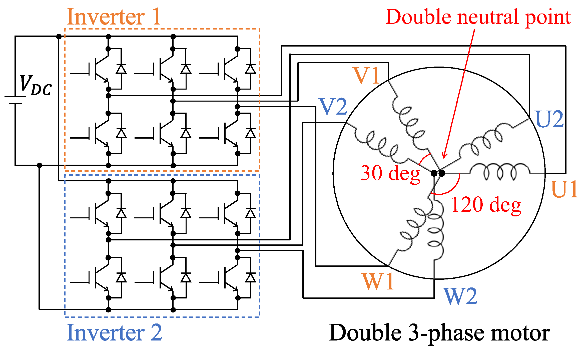
:1. Introduction
2. Coordinate System of Dual Three-Phase Motors
2.1. Stationary Orthogonal Subspaces
- k = 1, 13, 25, …, 12 m + 1 (m = 0, 1, 2, …):
- 2.
- k = 11, 23, 35, …, 12 m + 11 (m = 0, 1, 2, …):
- 3.
- k = 5, 17, 29, …, 12 m + 5 (m = 0, 1, 2, …):
- 4.
- k = 7, 19, 31, …, 12 m + 7 (m = 0, 1, 2, …):
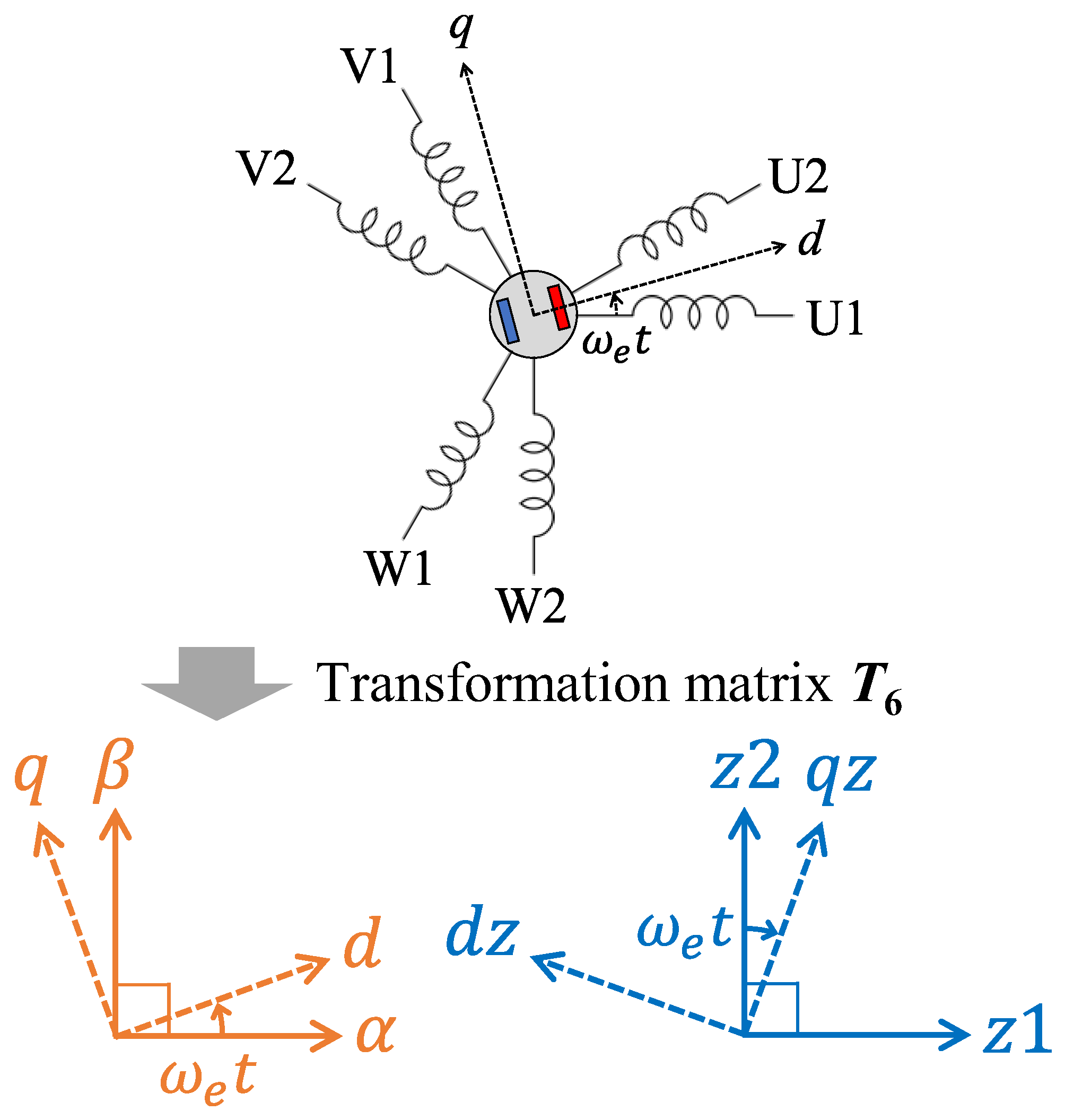
2.2. Rotational Orthogonal Subspaces
3. Mathematical Model of Dual Three-Phase IPMSM
3.1. Model with Inductance Saliency
3.2. Model Ignores Inductance Saliency
4. Design Method for Inductance of Dual Three-Phase Motors
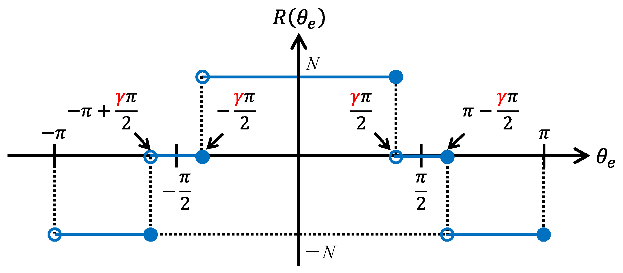
4.1. Definition of Winding Distribution Function
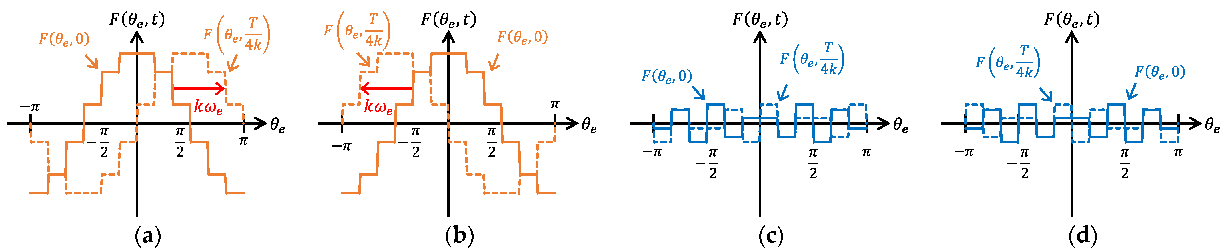
4.2. Magnetomotive Force Distribution for Harmonic Currents
- k = 1, 13, 25, …, 12 m + 1 (m = 0, 1, 2, …):
- 2.
- k = 11, 23, 35, …, 12 m + 11 (m = 0, 1, 2, …):
- 3.
- k = 5, 17, 29, …, 12 m + 5 (m = 0, 1, 2, …):
- 4.
- k = 7, 19, 31, …, 12 m + 7 (m = 0, 1, 2, …):
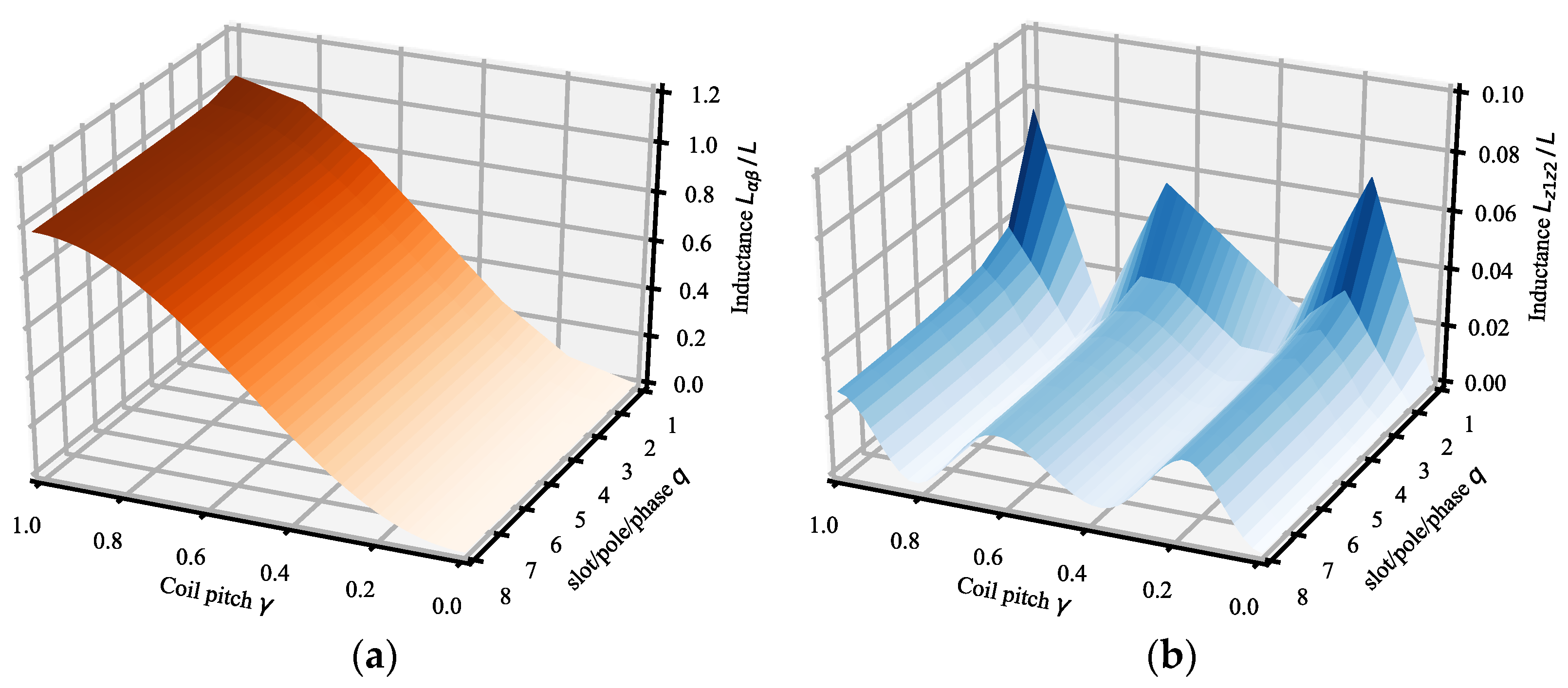
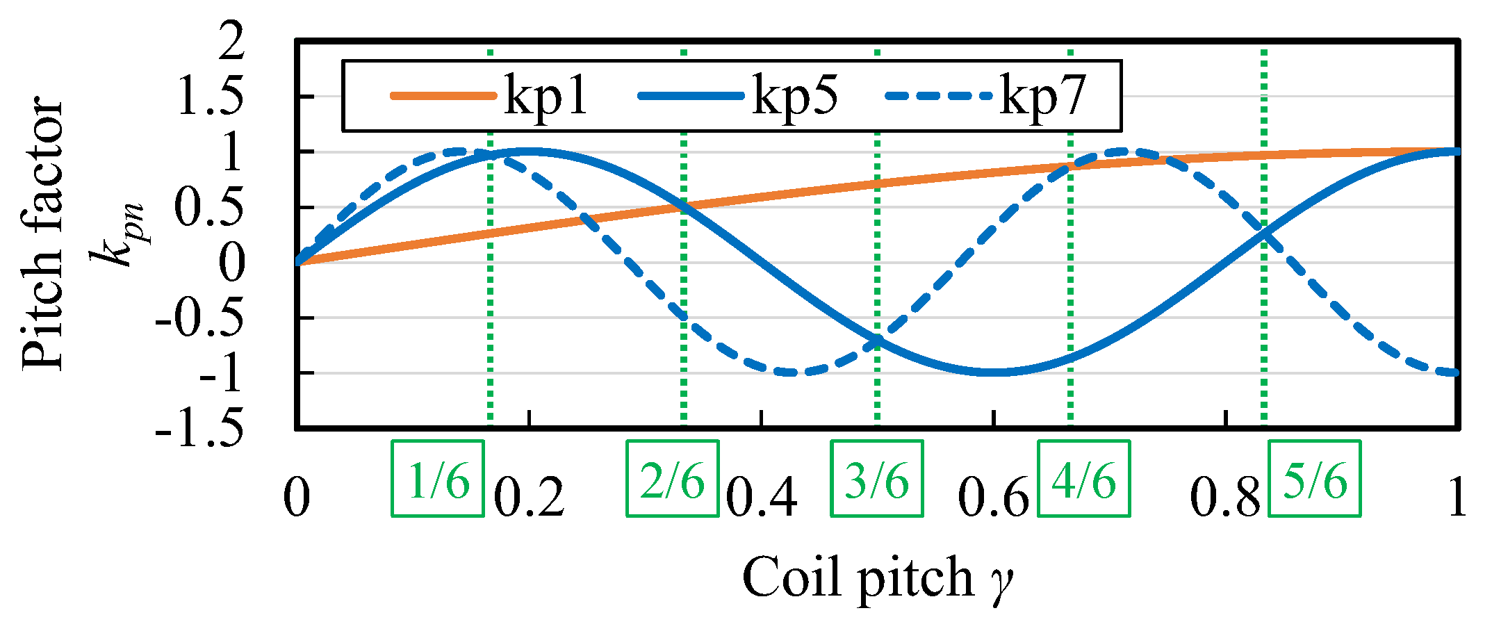
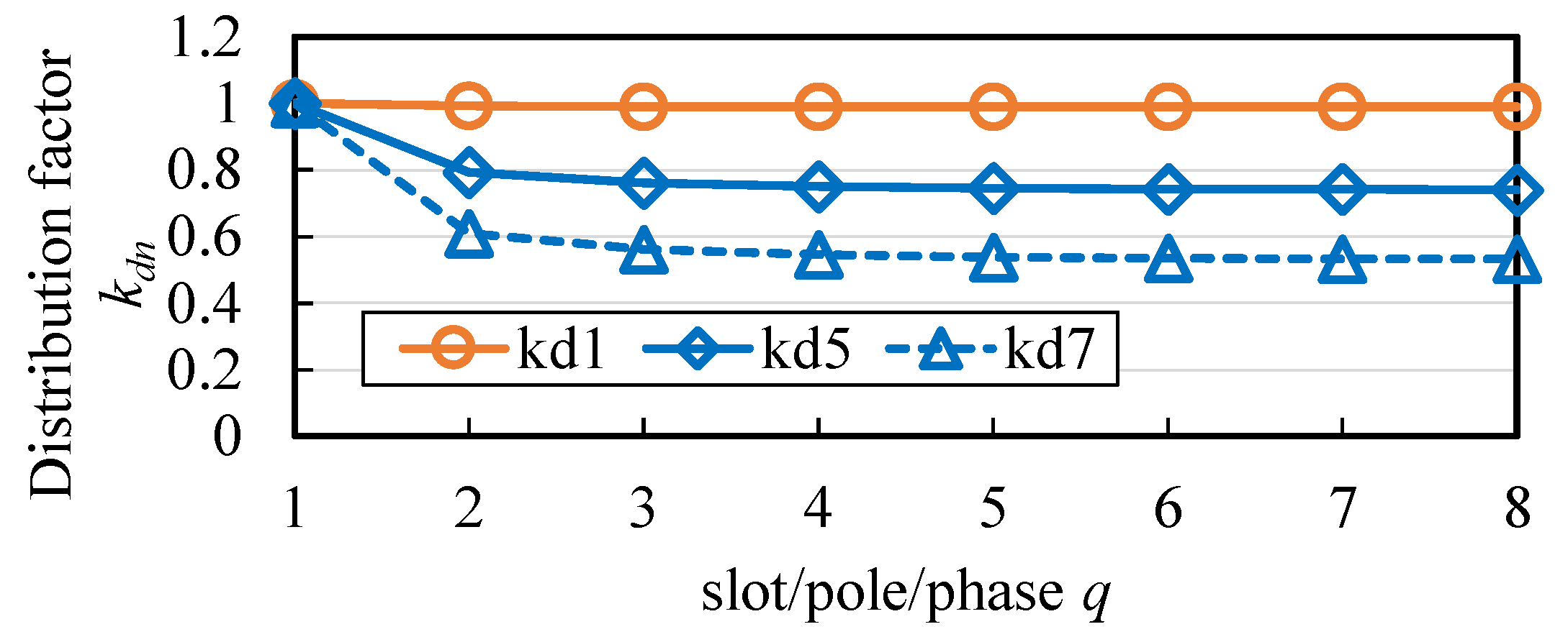
4.3. Calculation of Inductance
- k = 1, 13, 25, …, 12 m + 1 (m = 0, 1, 2, …):
- 2.
- k = 11, 23, 35, …, 12 m + 11 (m = 0, 1, 2, …):
- 3.
- k = 5, 17, 29, …, 12 m + 5 (m = 0, 1, 2, …):
- 4.
- k = 7, 19, 31, …, 12 m + 7 (m = 0, 1, 2, …):
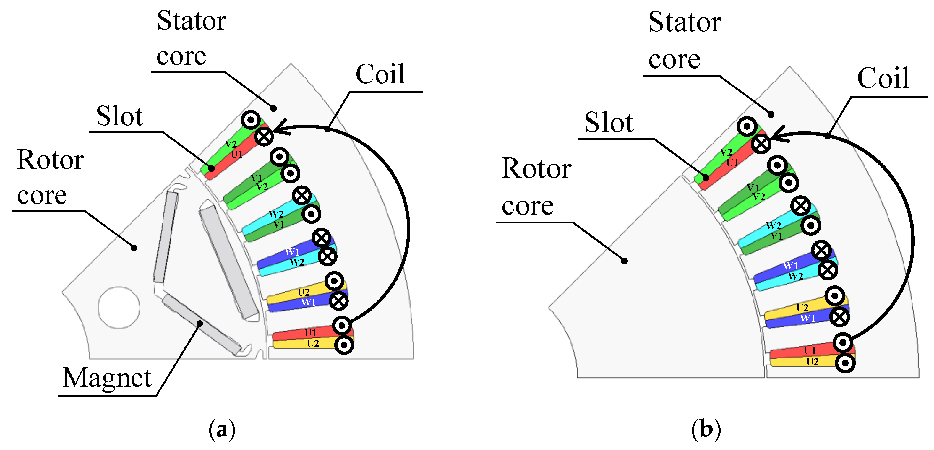
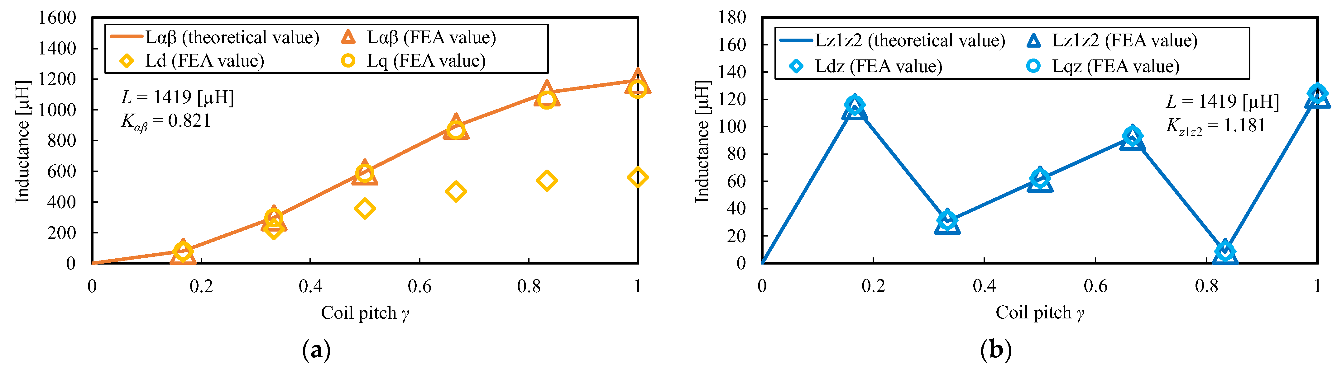
5. Verification by Finite Element Analysis
6. Verification by Circuit Simulation
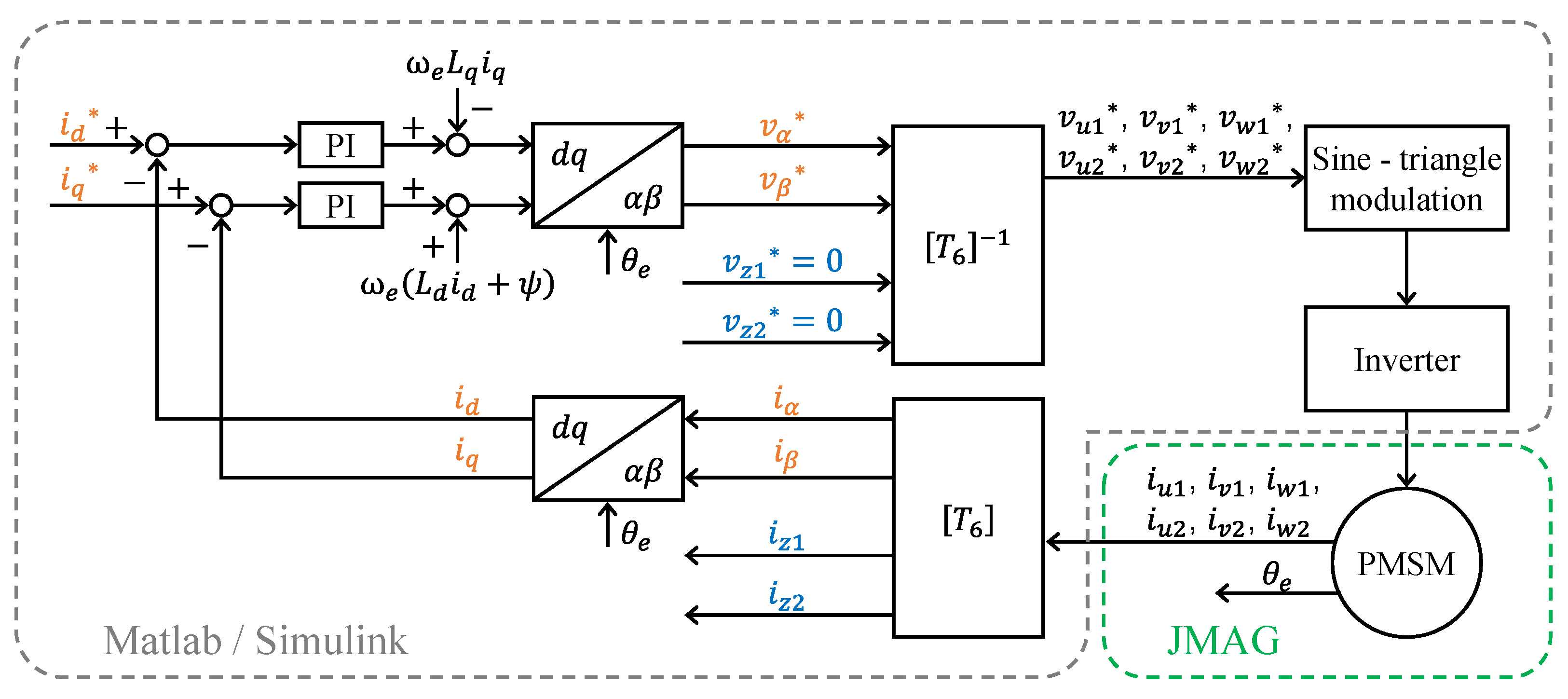
6.1. Simulation Method
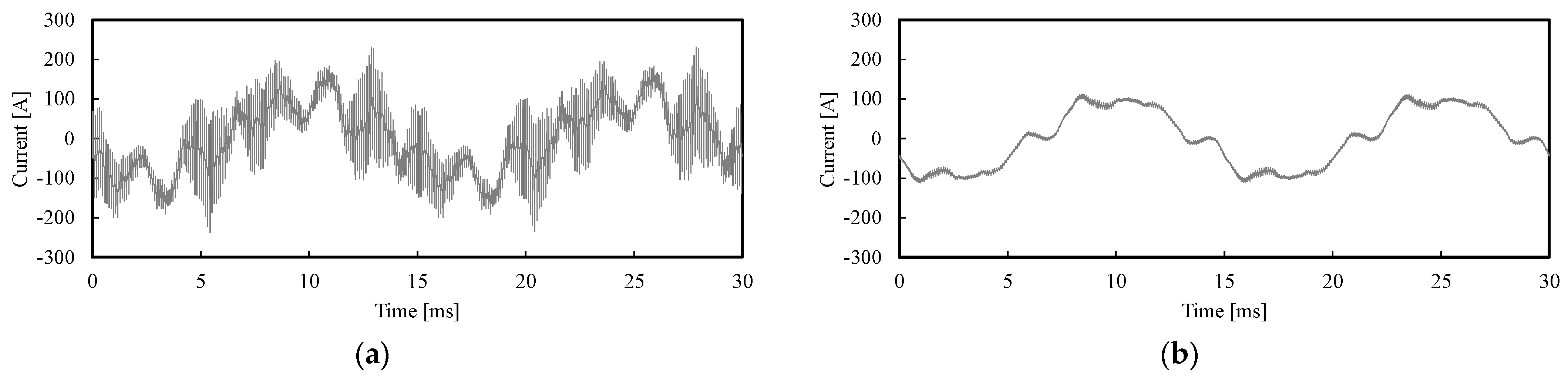
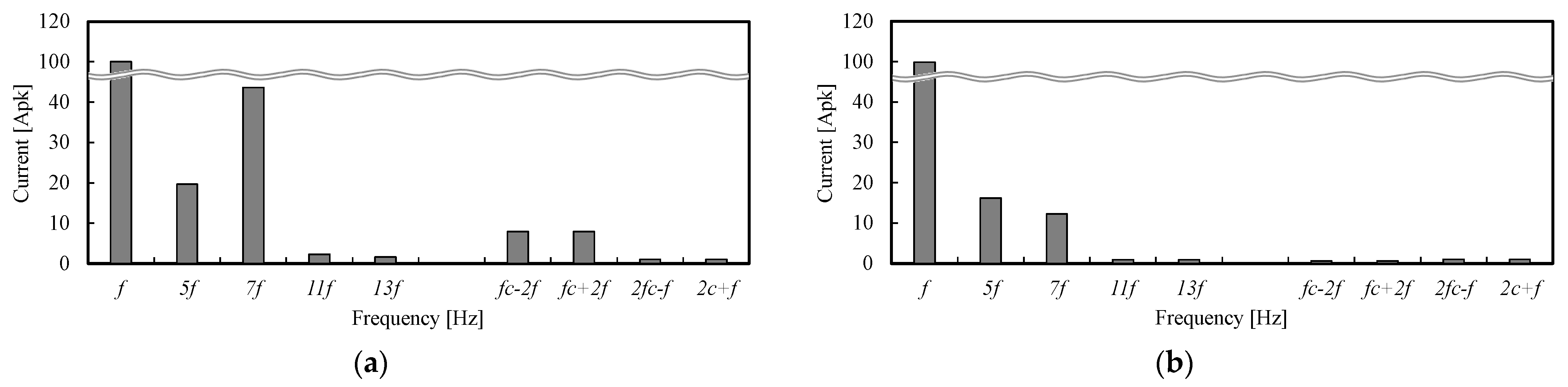
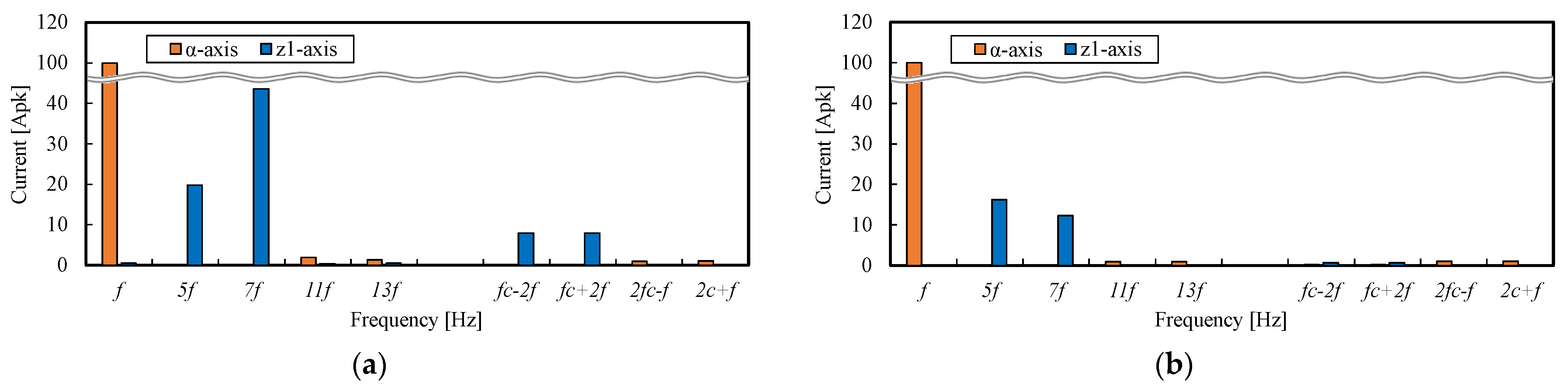
6.2. Simulation Results
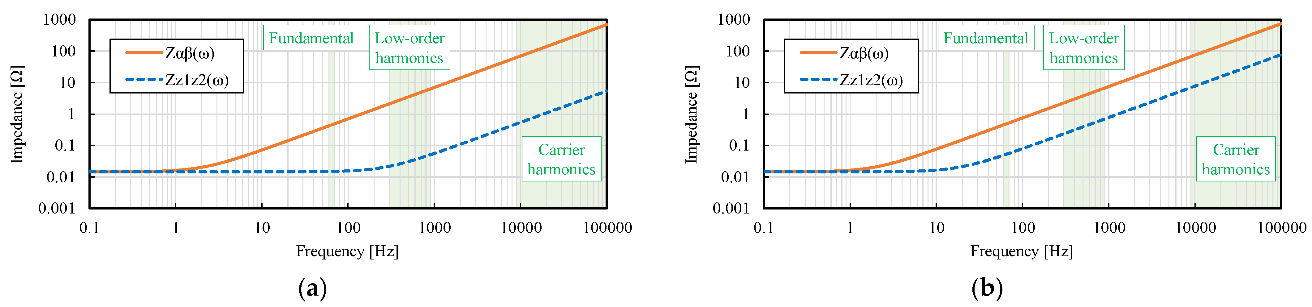
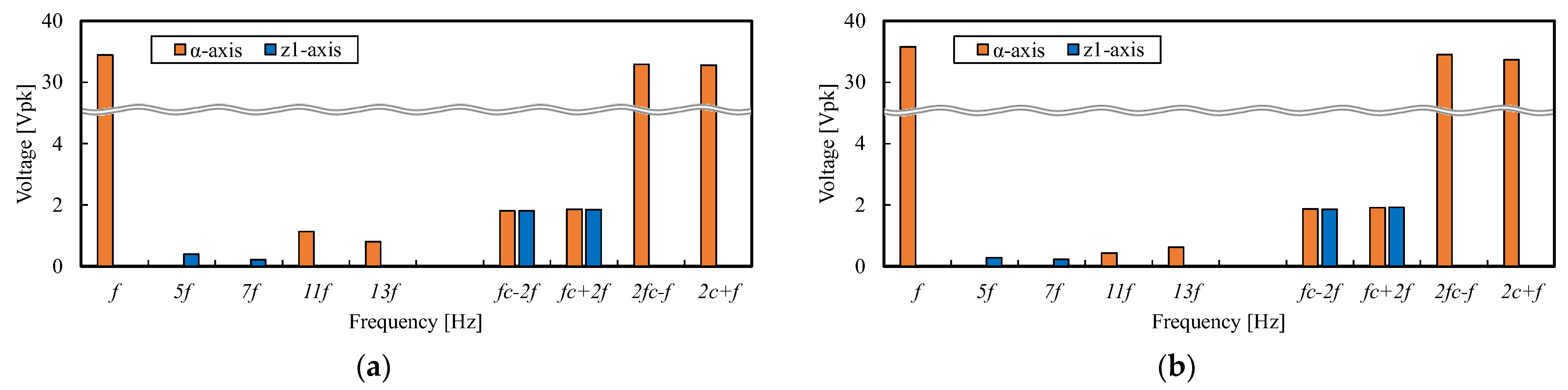
6.3. Consideration of the Relationship between the Magnitude of Harmonic Currents and Inductance Value
7. Conclusions
Author Contributions
Funding
Data Availability Statement
Conflicts of Interest
References
- Zhao, Y.; Lipo, T.A. Space vector PWM control of dual three-phase induction machine using vector space decomposition. IEEE Trans. Ind. Appl. 1995, 31, 1100–1109. [Google Scholar] [CrossRef]
- Marouani, K.; Baghli, L.; Hadiouche, D.; Kheloui, A.; Rezzoug, A. A New PWM Strategy Based on a 24-Sector Vector Space Decomposition for a Six-Phase VSI-Fed Dual Stator Induction Motor. IEEE Trans. Ind. Electron. 2008, 55, 1910–1920. [Google Scholar] [CrossRef]
- Yan, L.; Zhu, Z.Q.; Qi, J.; Ren, Y.; Gan, C.; Brockway, S.; Hilton, C. Suppression of Major Current Harmonics for Dual Three-Phase PMSMs by Virtual Multi Three-Phase Systems. IEEE Trans. Ind. Electron. 2022, 69, 5478–5490. [Google Scholar] [CrossRef]
- Hu, Y.; Zhu, Z.; Liu, K. Current Control for Dual Three-Phase Permanent Magnet Synchronous Motors Accounting for Current Unbalance and Harmonics. IEEE J. Emerg. Sel. Top. Power Electron. 2014, 2, 272–284. [Google Scholar]
- Hu, Y.; Zhu, Z.Q.; Odavic, M. Comparison of Two-Individual Current Control and Vector Space Decomposition Control for Dual Three-Phase PMSM. IEEE Trans. Ind. Appl. 2017, 53, 4483–4492. [Google Scholar] [CrossRef]
- Hadiouche, D.; Razik, H.; Rezzoug, A. On the modeling and design of dual-stator windings to minimize circulating harmonic currents for VSI fed AC machines. IEEE Trans. Ind. Appl. 2004, 40, 506–515. [Google Scholar] [CrossRef]
- Ye, D.; Li, J.; Qu, R.; Jiang, D.; Xiao, L.; Lu, Y.; Chen, J. Variable Switching Sequence PWM Strategy of Dual Three-Phase Machine Drive for High-Frequency Current Harmonic Suppression. IEEE Trans. Power Electron. 2020, 35, 4984–4995. [Google Scholar] [CrossRef]
- Kallio, S.; Andriollo, M.; Tortella, A.; Karttunen, J. Decoupled d-q Model of Double-Star Interior-Permanent-Magnet Synchronous Machines. IEEE Trans. Ind. Electron. 2013, 60, 2486–2494. [Google Scholar] [CrossRef]
- Okajima, Y.; Akatsu, K. Complex Vector form PI Control for Harmonic Current Control of a PMSM. IEEJ Trans. Ind. Appl. 2017, 137, 238–245. [Google Scholar] [CrossRef]


| Harmonic Order k | 1 | 3 | 5 | 7 | 9 | 11 | 13 | … |
|---|---|---|---|---|---|---|---|---|
| Conventional 3-phase motor | α-β Positive sequence | Zero sequence | α-β Negative sequence | α-β Positive sequence | Zero sequence | α-β Negative sequence | α-β Positive sequence | … |
| Dual 3-phase motor | α-β Positive sequence | o1-o2 Zero sequence | z1-z2 Positive sequence | z1-z2 Negative sequence | o1-o2 Zero sequence | α-β Negative sequence | α-β Positive sequence | … |
| Parameter | Value |
|---|---|
| Number of poles | 8 |
| Number of slots | 48 |
| Stator inner diameter r [mm] | 131 |
| Stack length l [mm] | 141 |
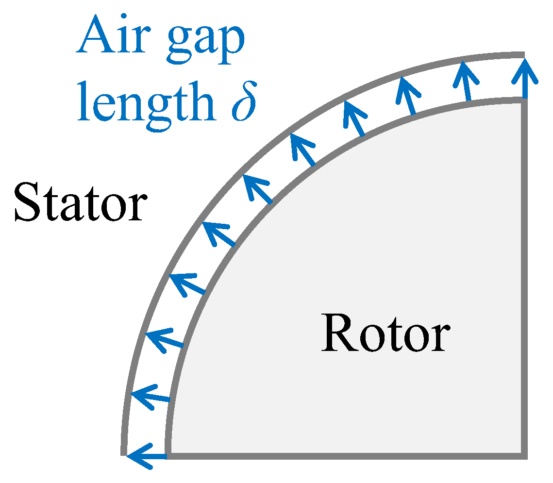
| Air gap length δ [mm] | 0.5 |
| Number of turns N | 4 |
| Number of parallels in circuit b | 2 |
| Parameter | Value |
|---|---|
| Reference current [Apk] | 100 |
| Fundamental electrical frequency f [Hz] | 66.67 |
| Carrier frequency fc [Hz] | 10,000 |
| DC voltage [V] | 365 |
Disclaimer/Publisher’s Note: The statements, opinions and data contained in all publications are solely those of the individual author(s) and contributor(s) and not of MDPI and/or the editor(s). MDPI and/or the editor(s) disclaim responsibility for any injury to people or property resulting from any ideas, methods, instructions or products referred to in the content. |
© 2023 by the authors. Licensee MDPI, Basel, Switzerland. This article is an open access article distributed under the terms and conditions of the Creative Commons Attribution (CC BY) license (https://creativecommons.org/licenses/by/4.0/).
Share and Cite
Yoshida, A.; Akatsu, K. Study of Winding Structure to Reduce Harmonic Currents in Dual Three-Phase Motor. World Electr. Veh. J. 2023, 14, 100. https://doi.org/10.3390/wevj14040100
Yoshida A, Akatsu K. Study of Winding Structure to Reduce Harmonic Currents in Dual Three-Phase Motor. World Electric Vehicle Journal. 2023; 14(4):100. https://doi.org/10.3390/wevj14040100
Chicago/Turabian StyleYoshida, Akito, and Kan Akatsu. 2023. "Study of Winding Structure to Reduce Harmonic Currents in Dual Three-Phase Motor" World Electric Vehicle Journal 14, no. 4: 100. https://doi.org/10.3390/wevj14040100