

Adaptive Nonlinear Control of Salient-Pole PMSM for Hybrid Electric Vehicle Applications: Theory and Experiments
 , , , and
Abstract
:1. Introduction
2. SP-PMSM Mathematic Model
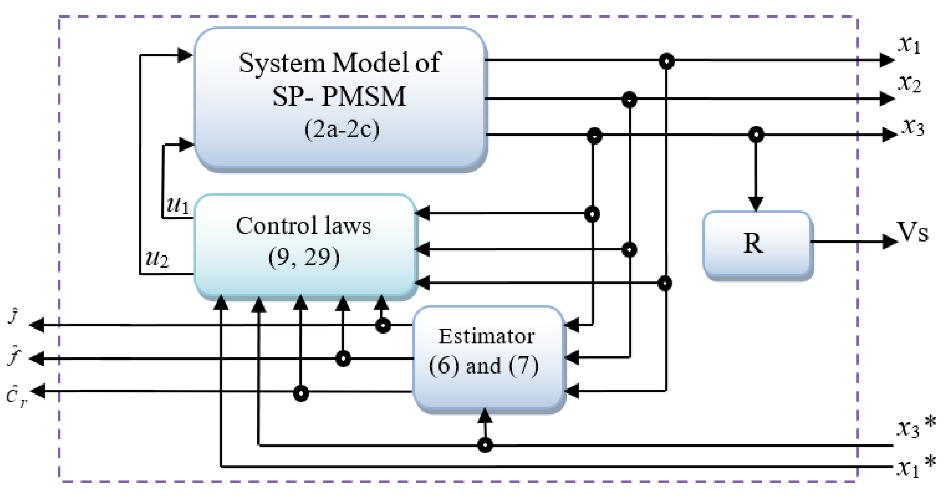
- Controlling the signals and to their references;
- Estimating the non-measurable parameters of a SP-PMSM, such us and ;
- Estimating the load torque .
3. Adaptive Nonlinear Control
3.1. Adaptive Backstepping Design
3.2. Current-Controller Design Technique
3.3. Speed-Controller Design Technique
- Closed-loop system is GAS;
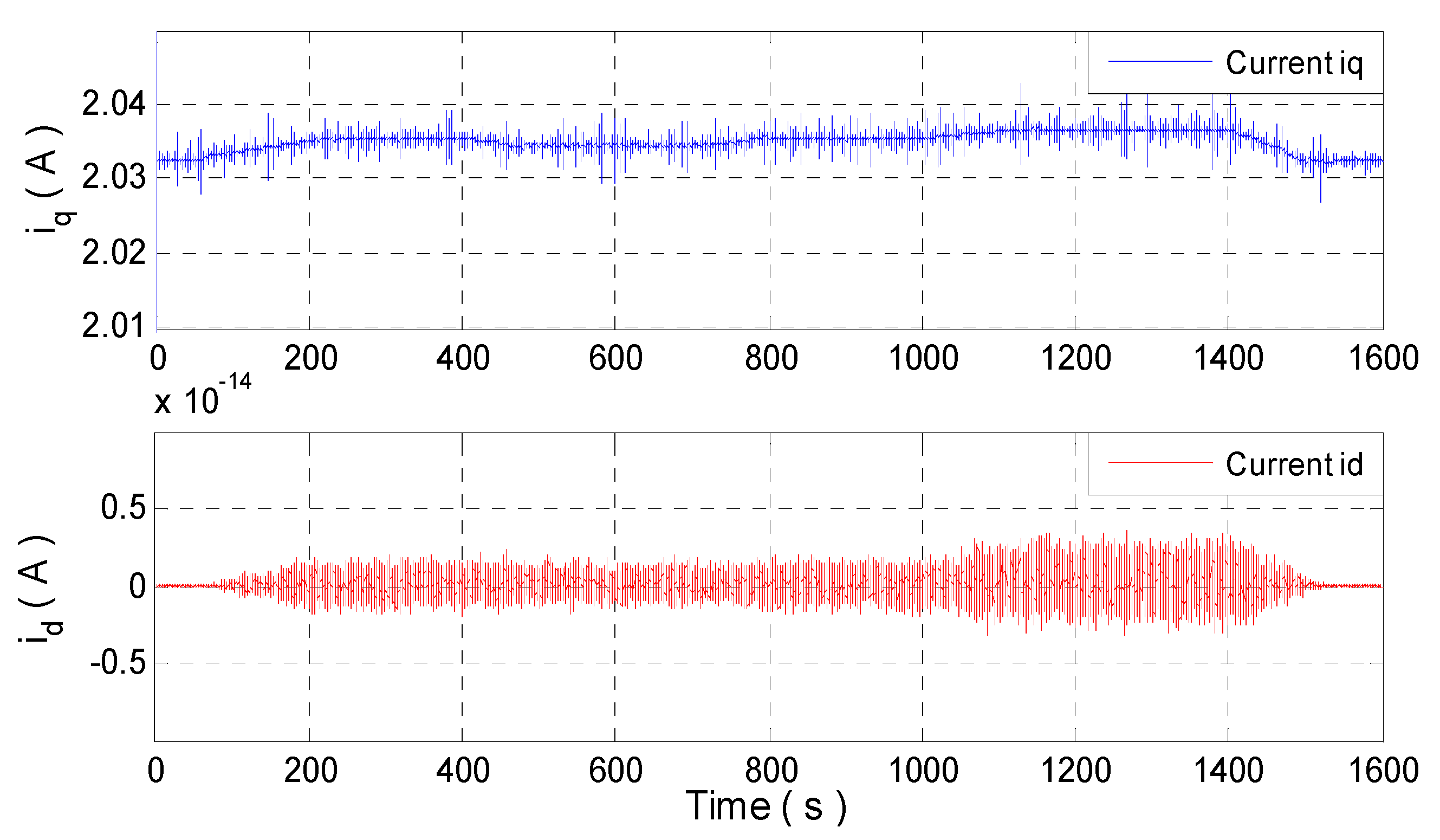
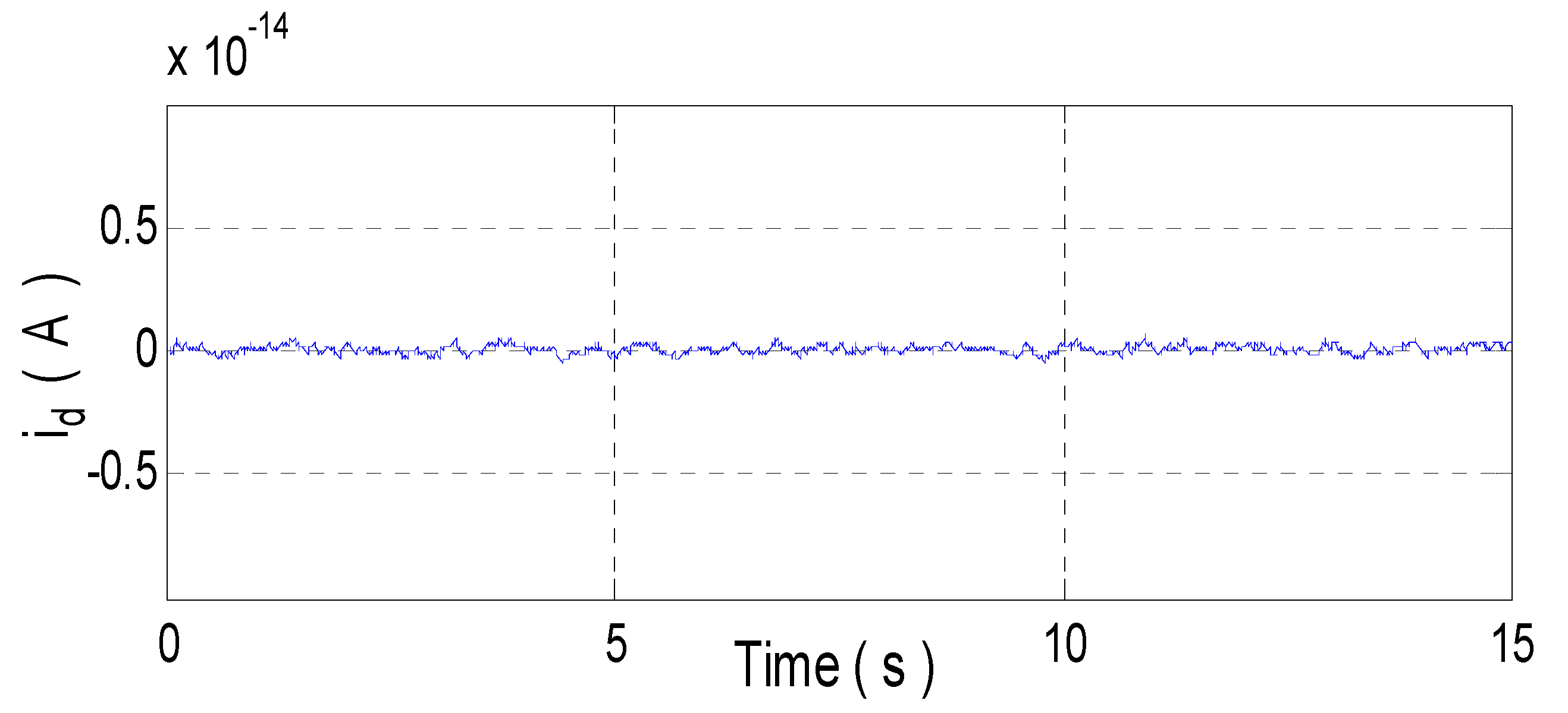
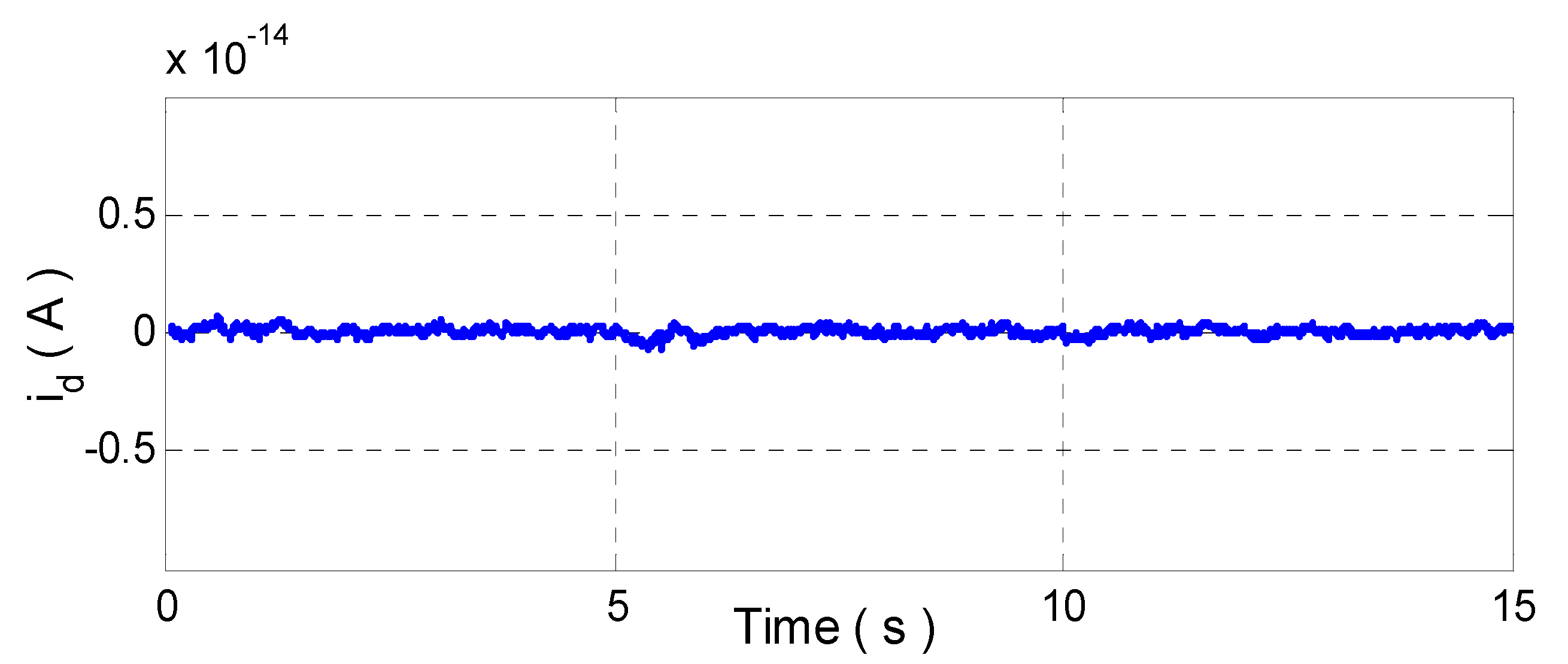
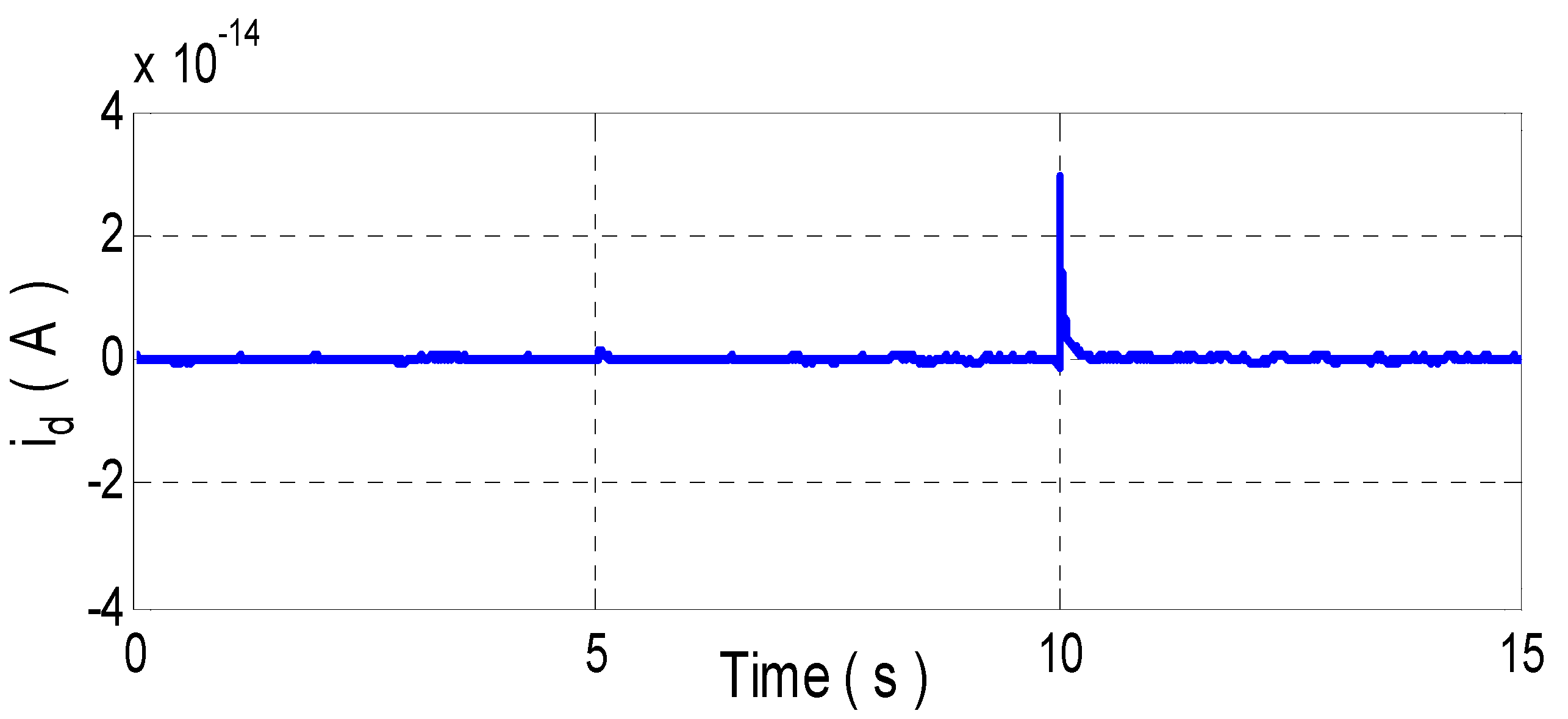
- Current d-axis regulation is set to zero;
- Perfect tracking of motor speed is set to its reference;
- Non-measurable parameters of the SP-PMSM such as f and J are estimated;
- Load torque Cr is estimated.
4. Numerical Simulation
4.1. Speed Change
- -
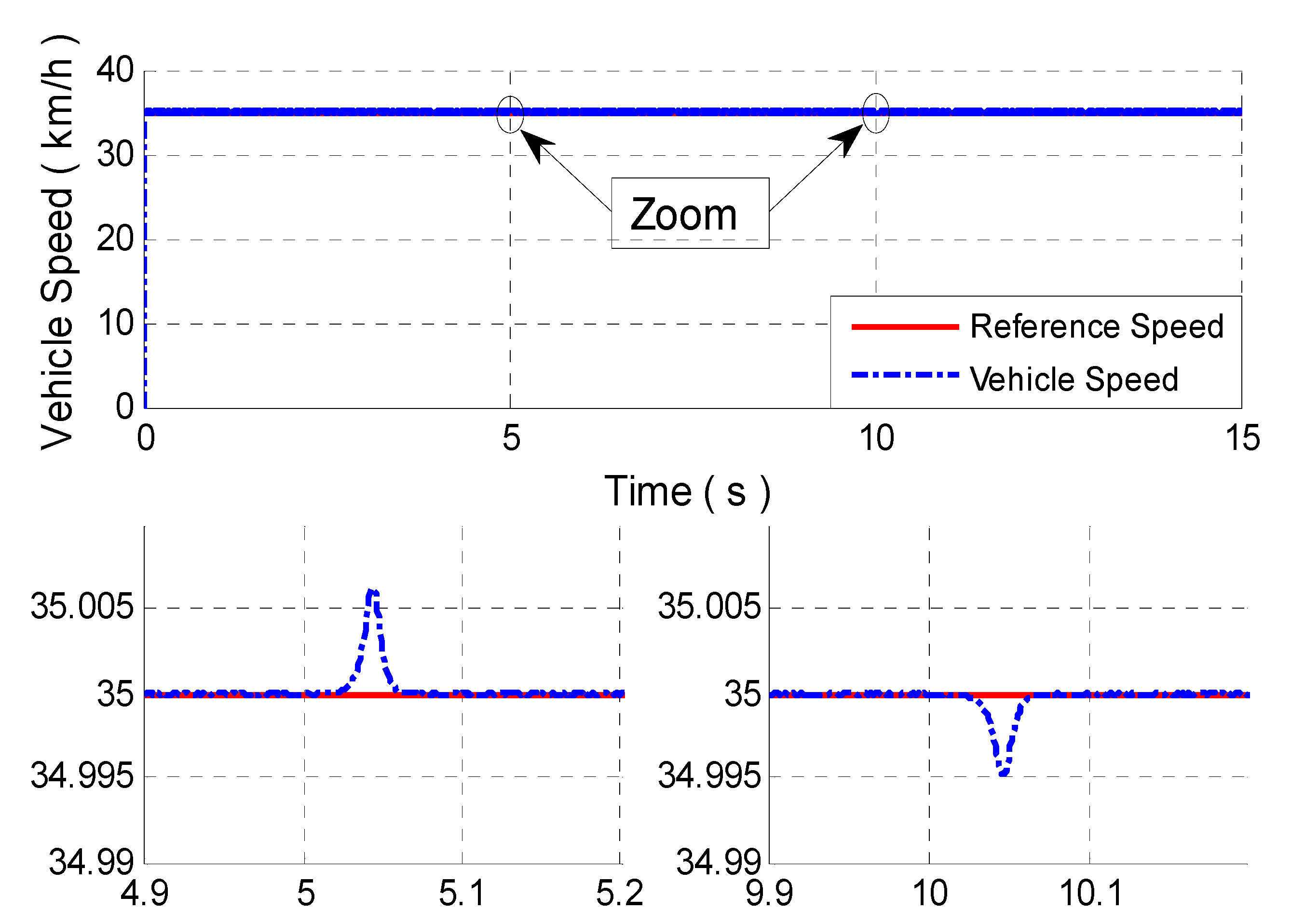
- The proposed control guarantees perfect vehicle speed tracking to its reference;
- -
- The closed-loop system is stable with respect to the variation in the reference speed.
4.2. Inertia Change
- -
- The perfect tracking of the vehicle speed to its reference;
- -
- The estimation of inertia J by this controller helps to ensure the stability and robustness of the system;
- -
- The moment of inertia J depends on the mass but not on the speed.
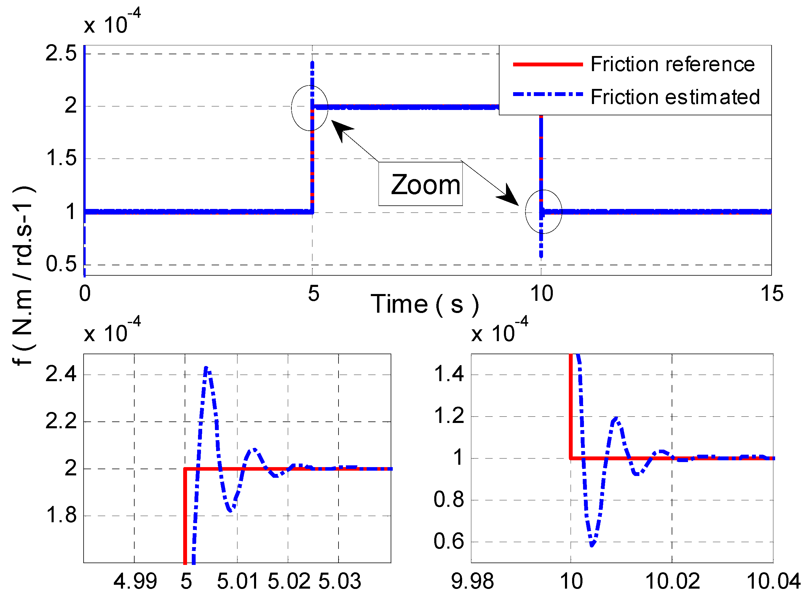
4.3. Friction Change
- -
- The perfect tracking of the vehicle speed to its reference;
- -
- The estimation of friction f by this controller helps to ensure the stability and robustness of the system;
- -
- The variation in friction due to the aging of the machine or in cases where the maintenance schedule of the machine is not maintained.
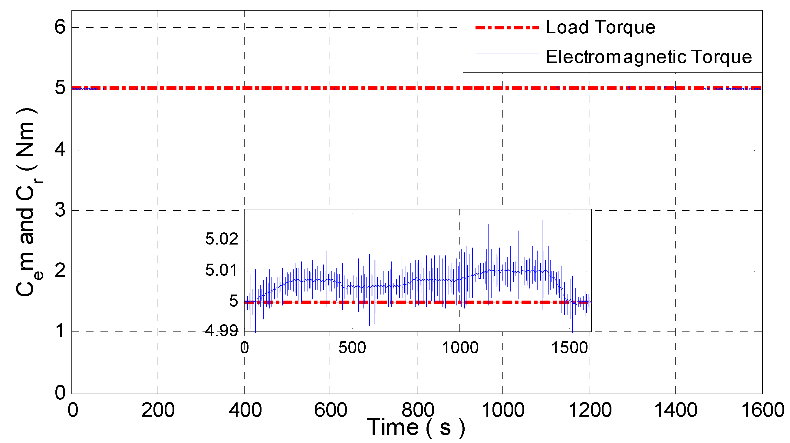
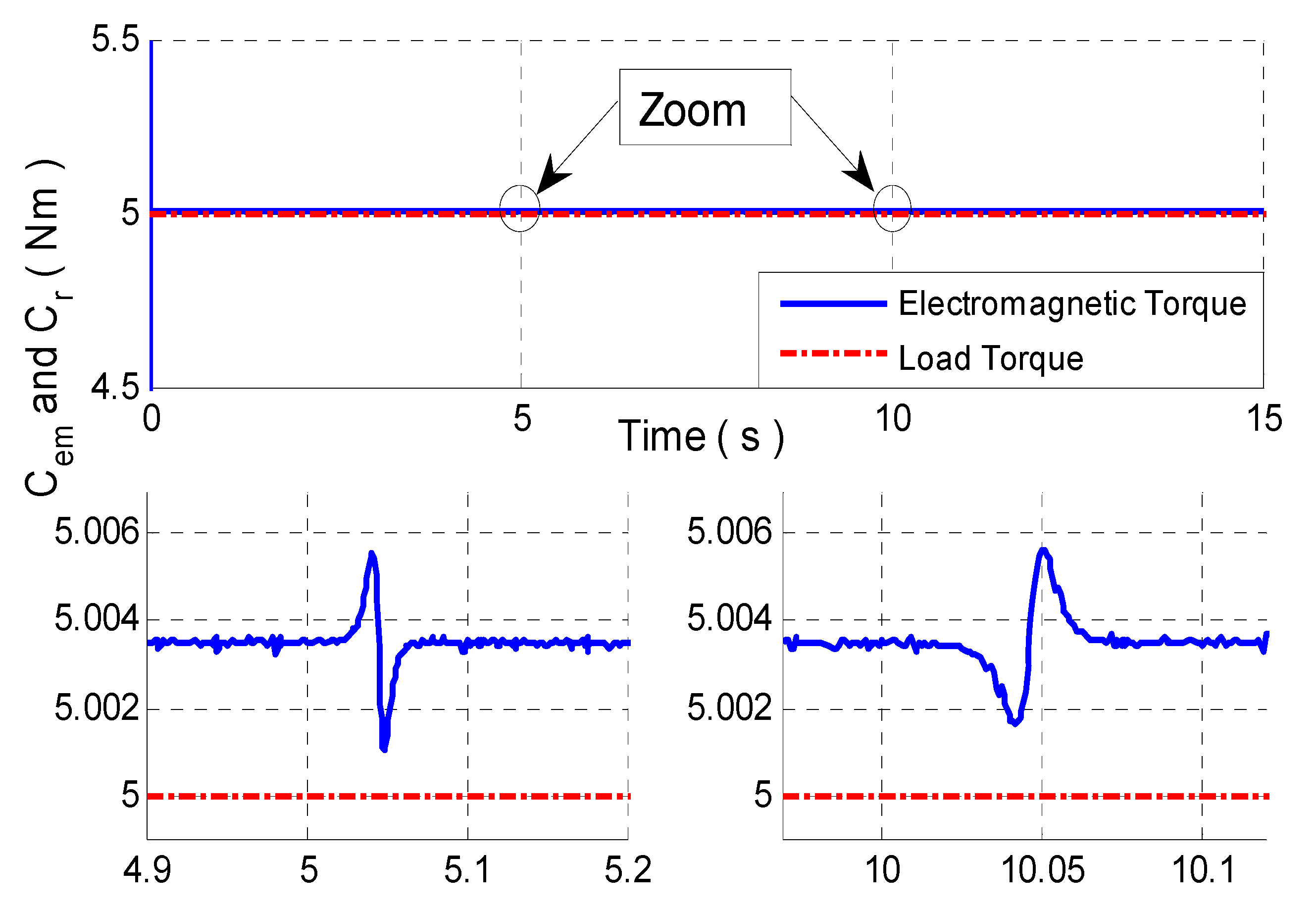
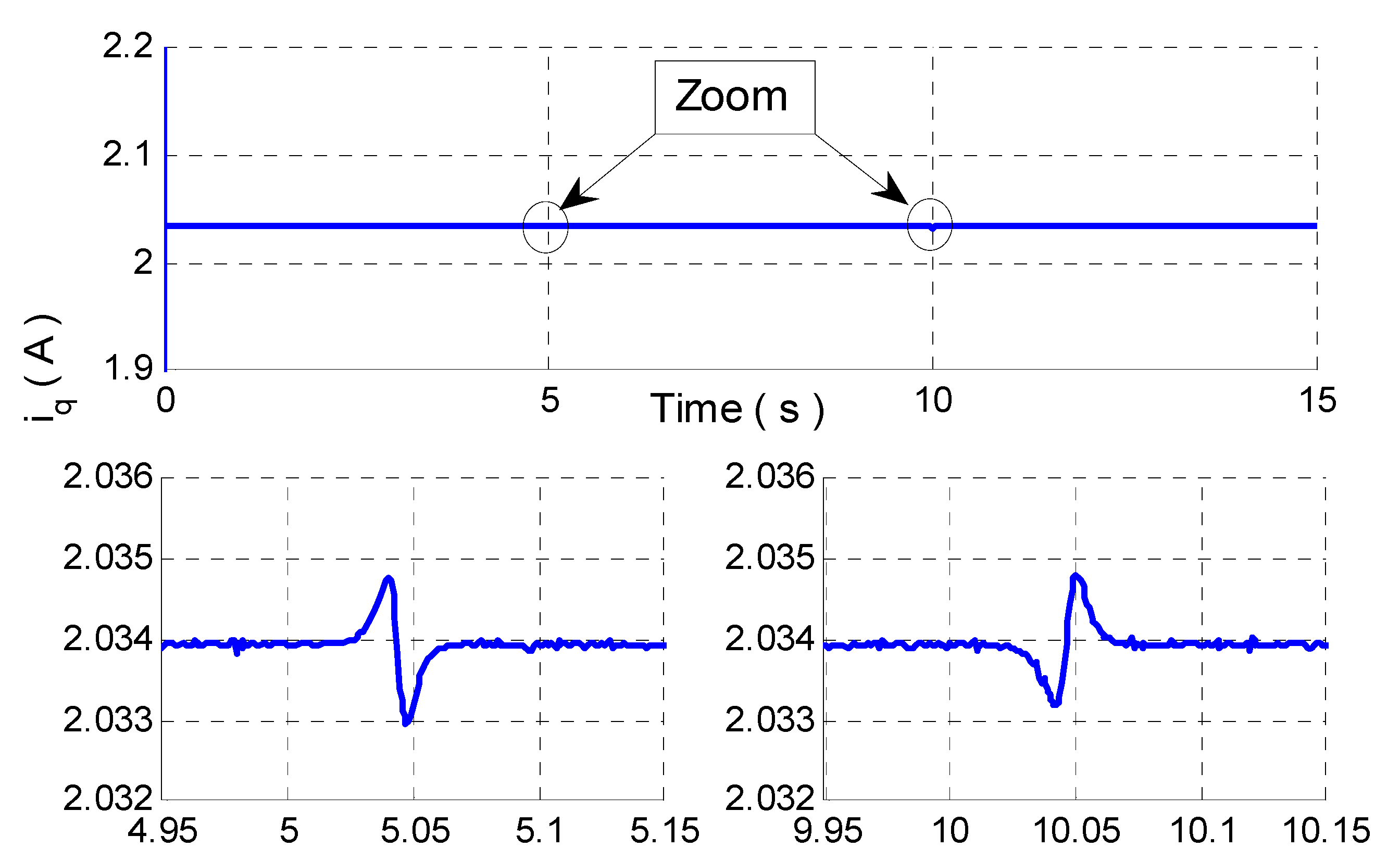
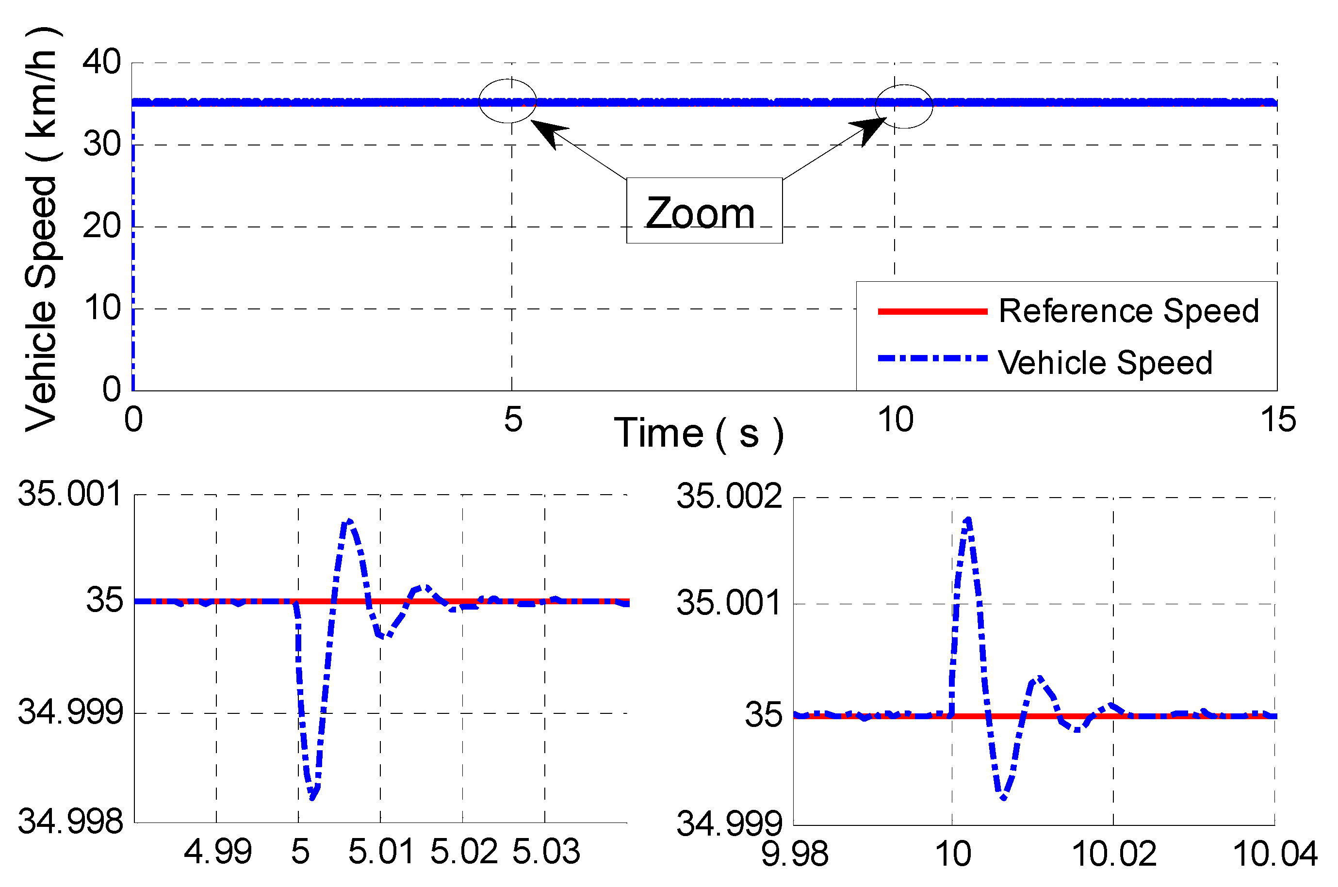
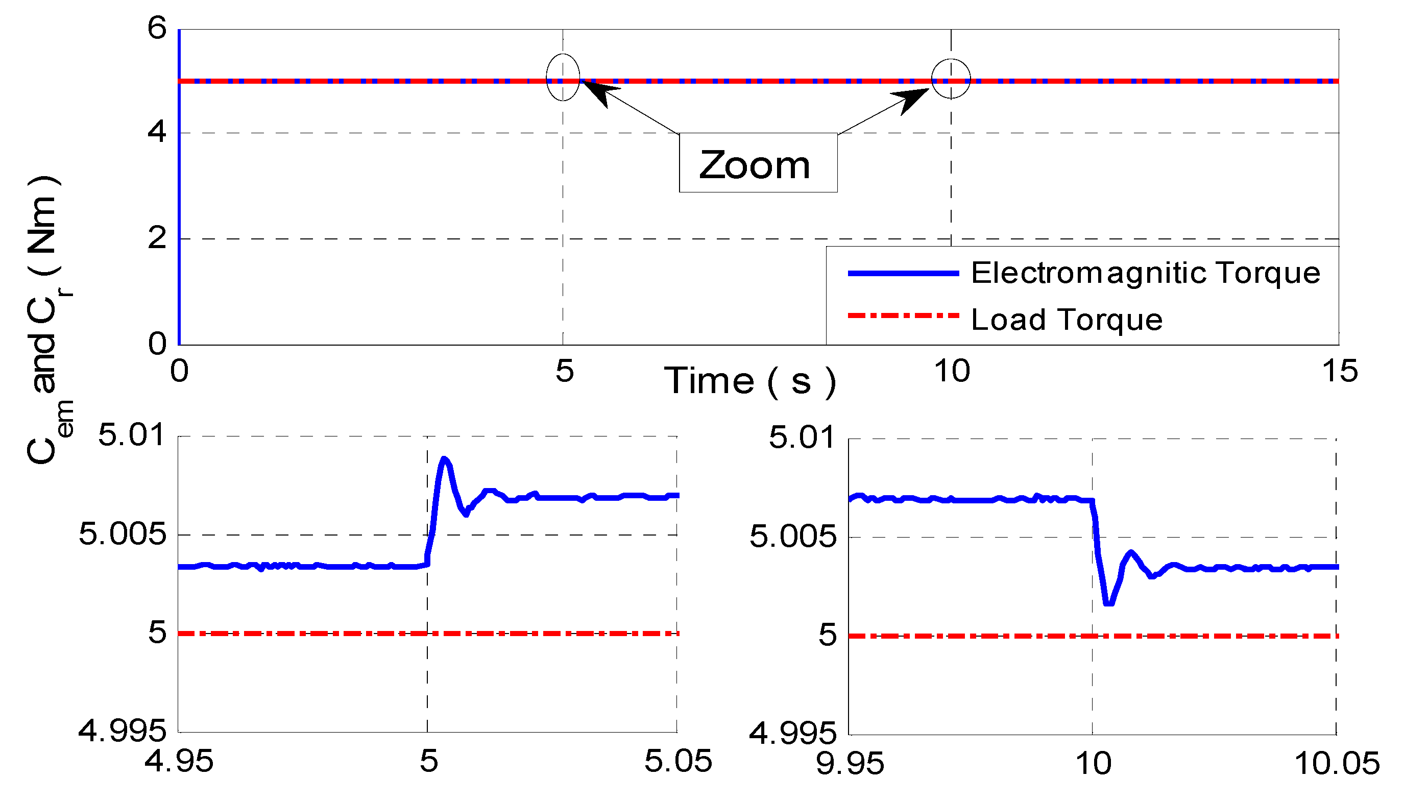
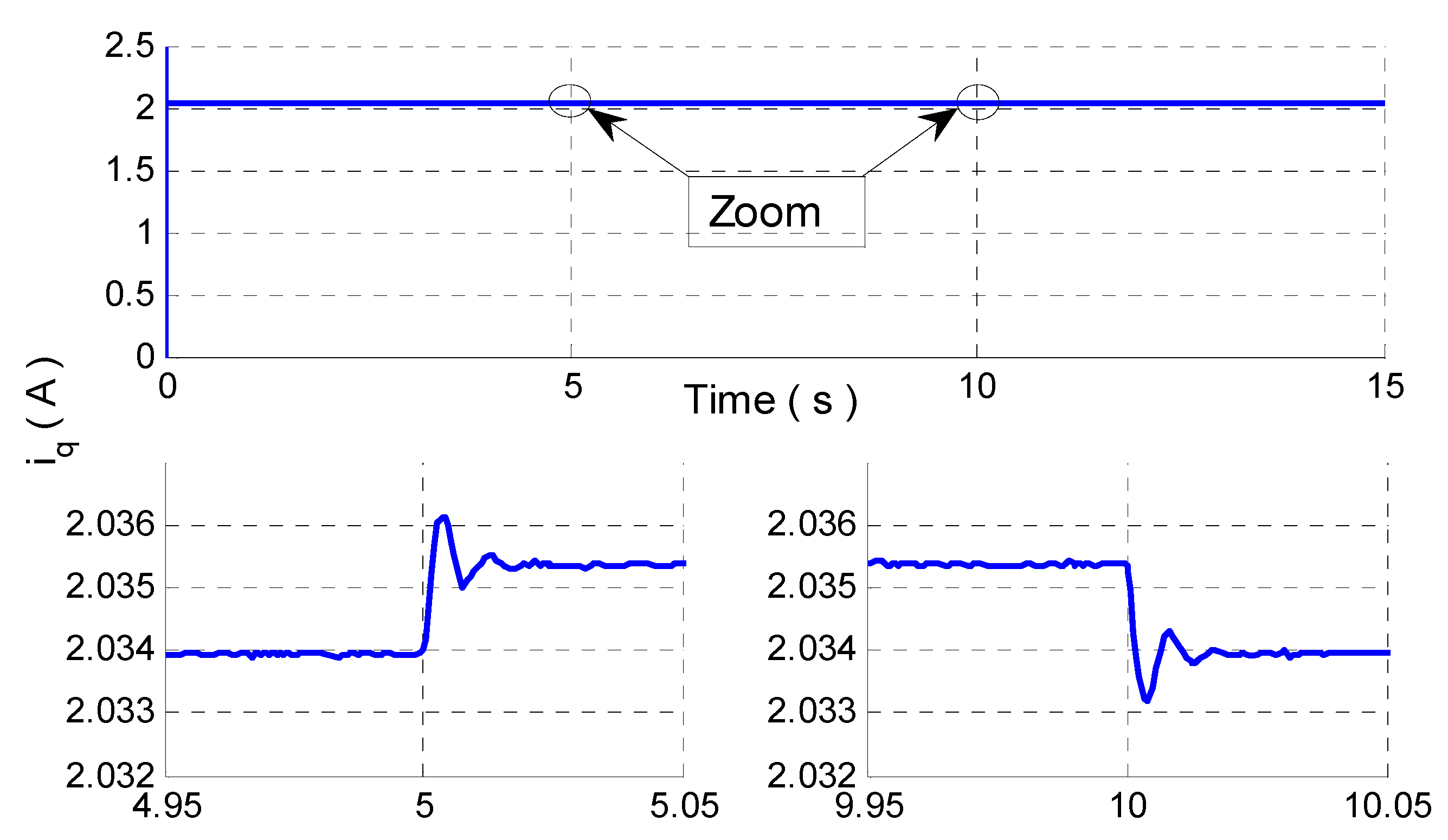
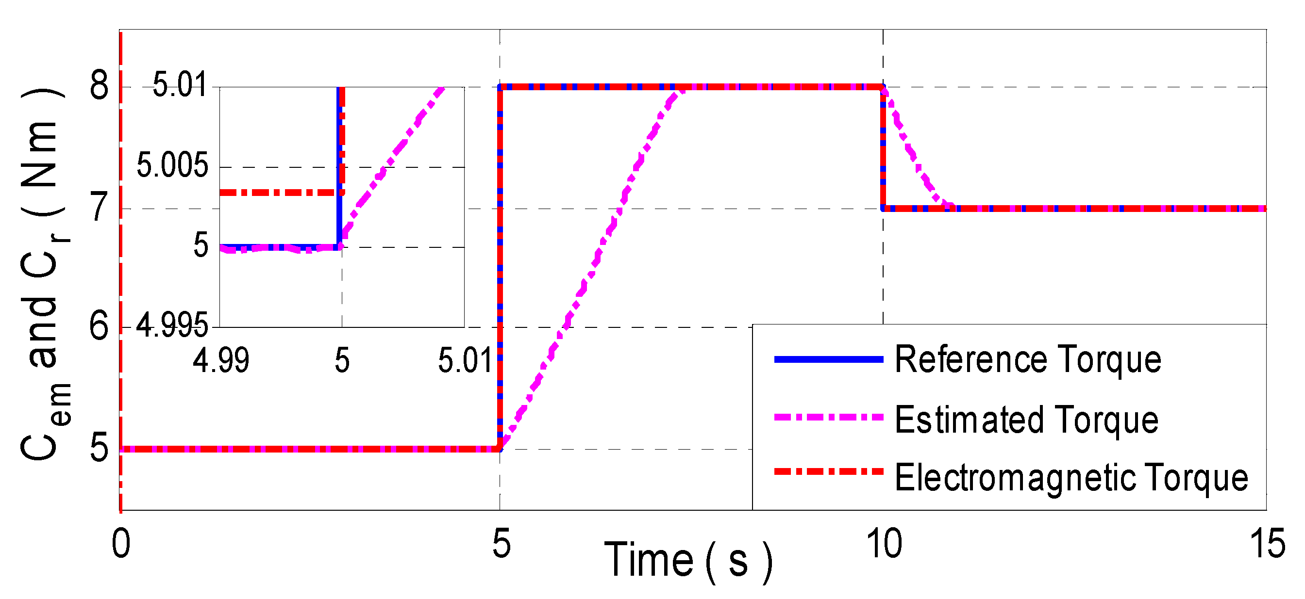
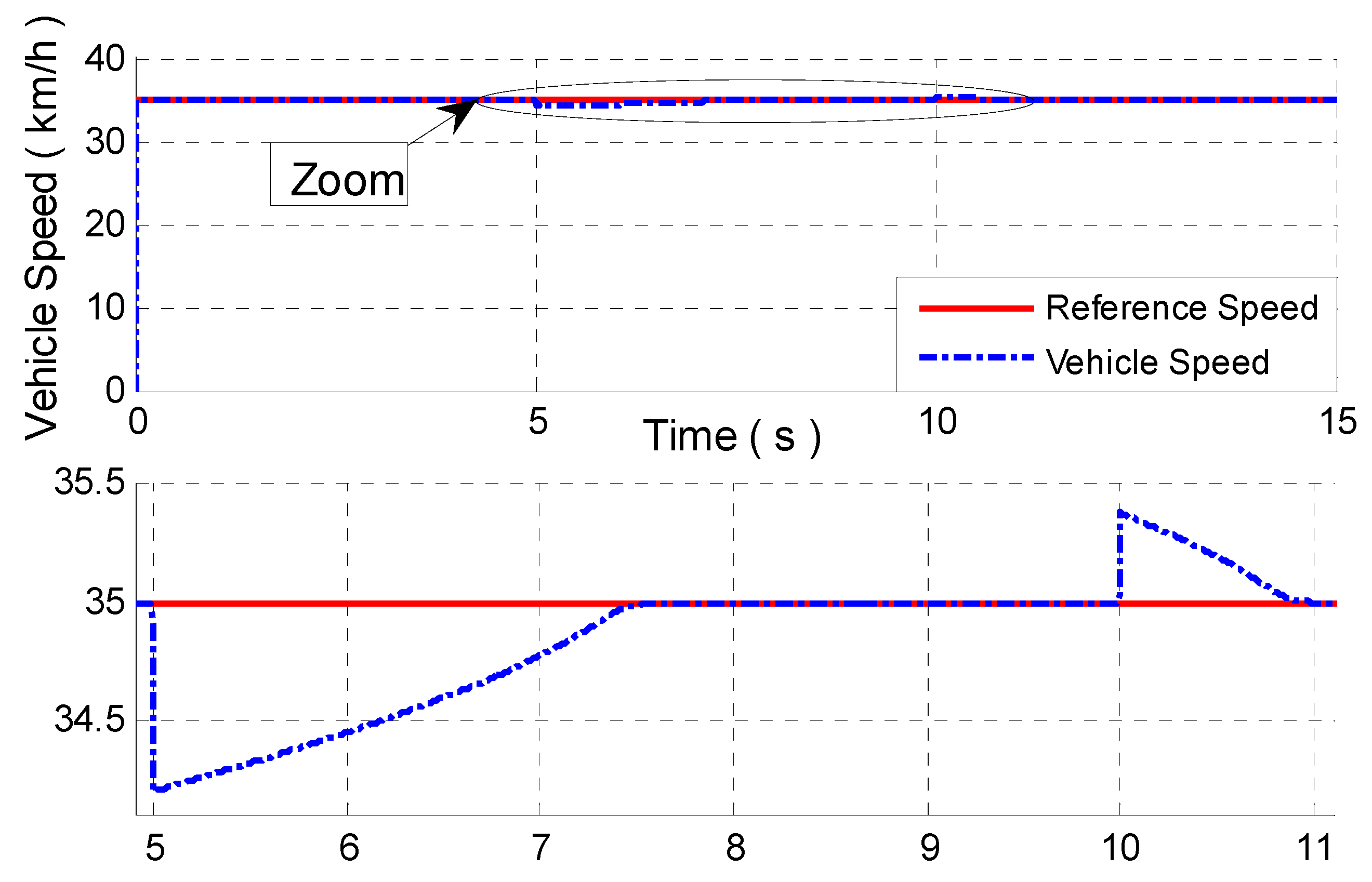
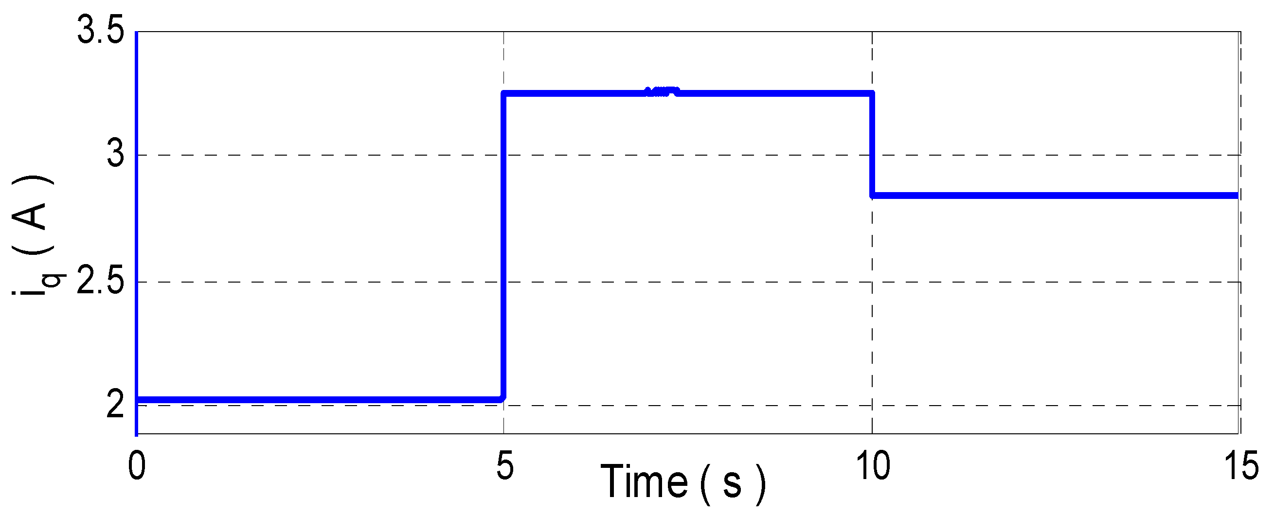
4.4. Torque Change
- -
- The perfect tracking of the vehicle speed to its reference;
- -
- The estimation of Cr by this controller helps to ensure the stability and robustness of the system.
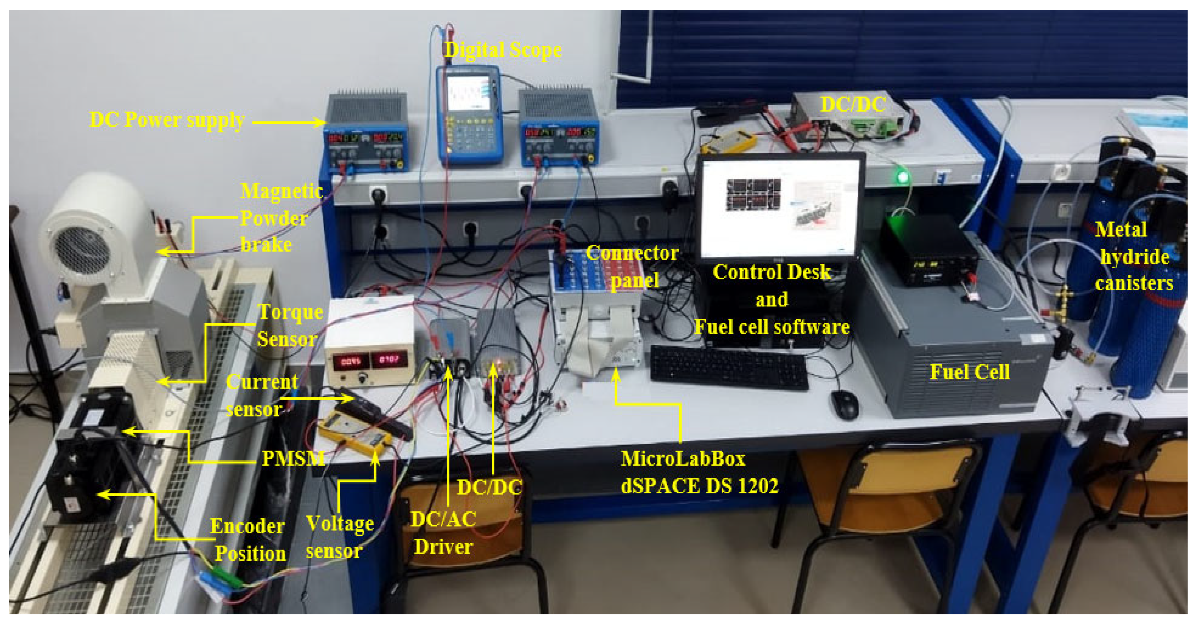
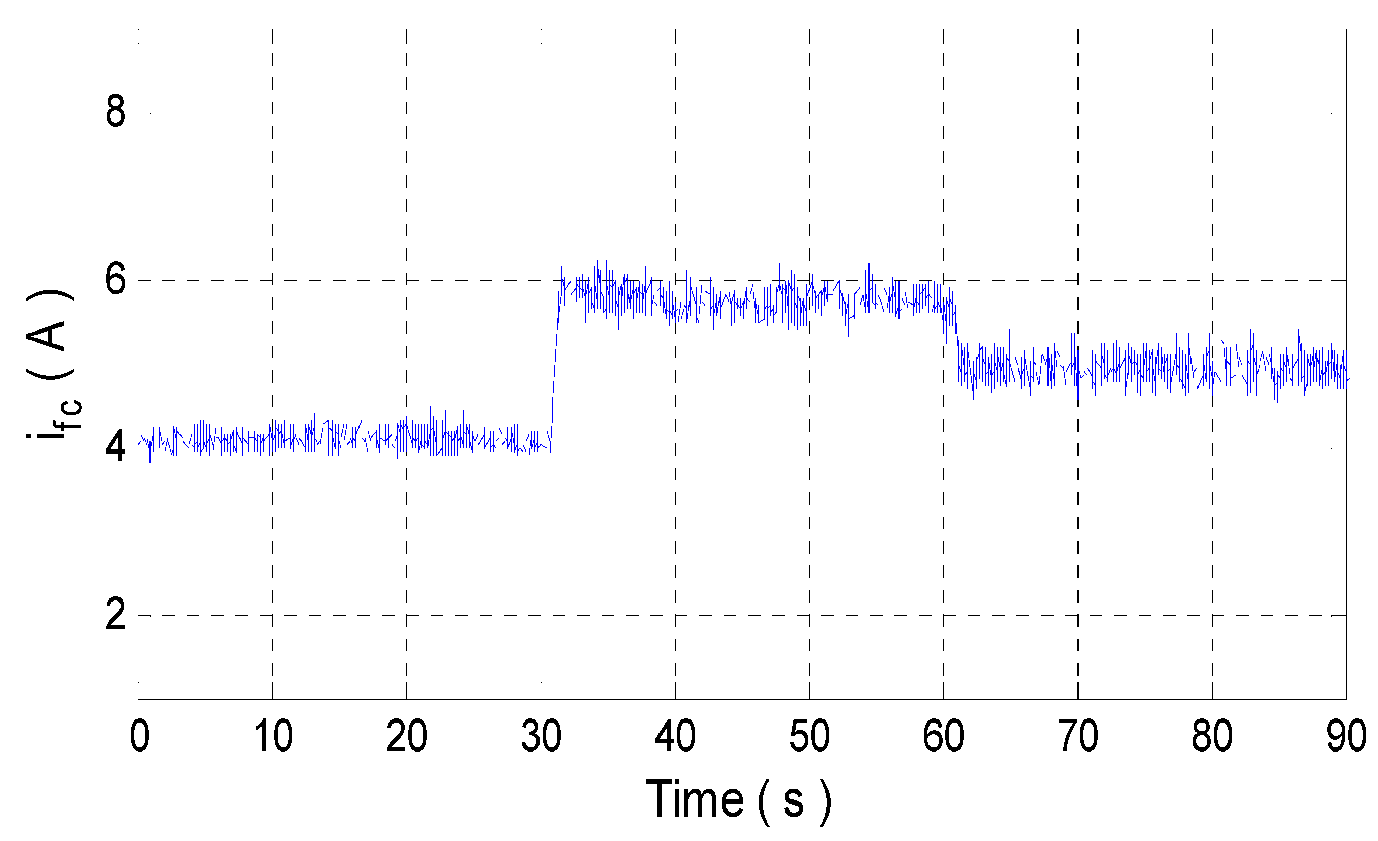
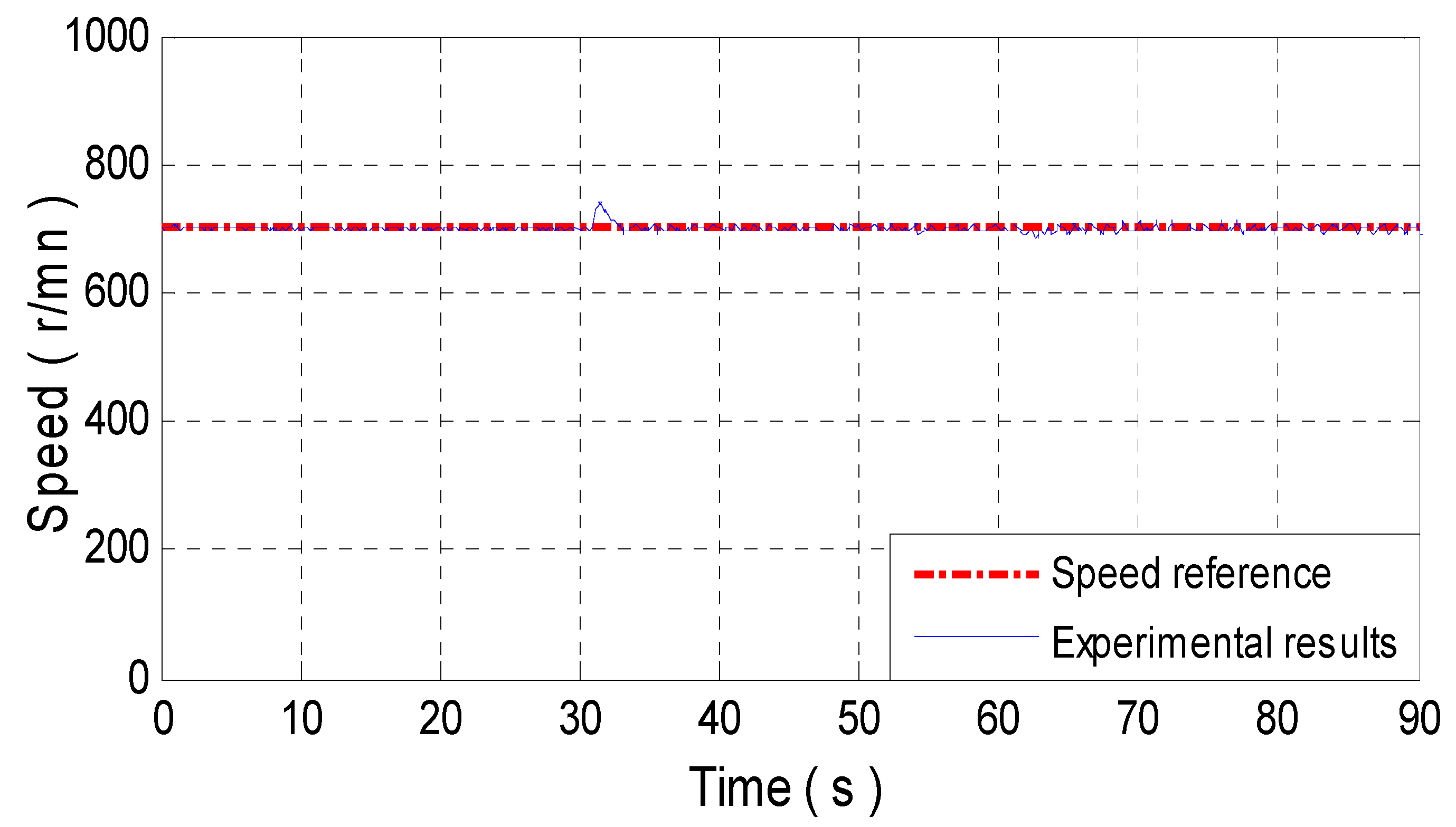
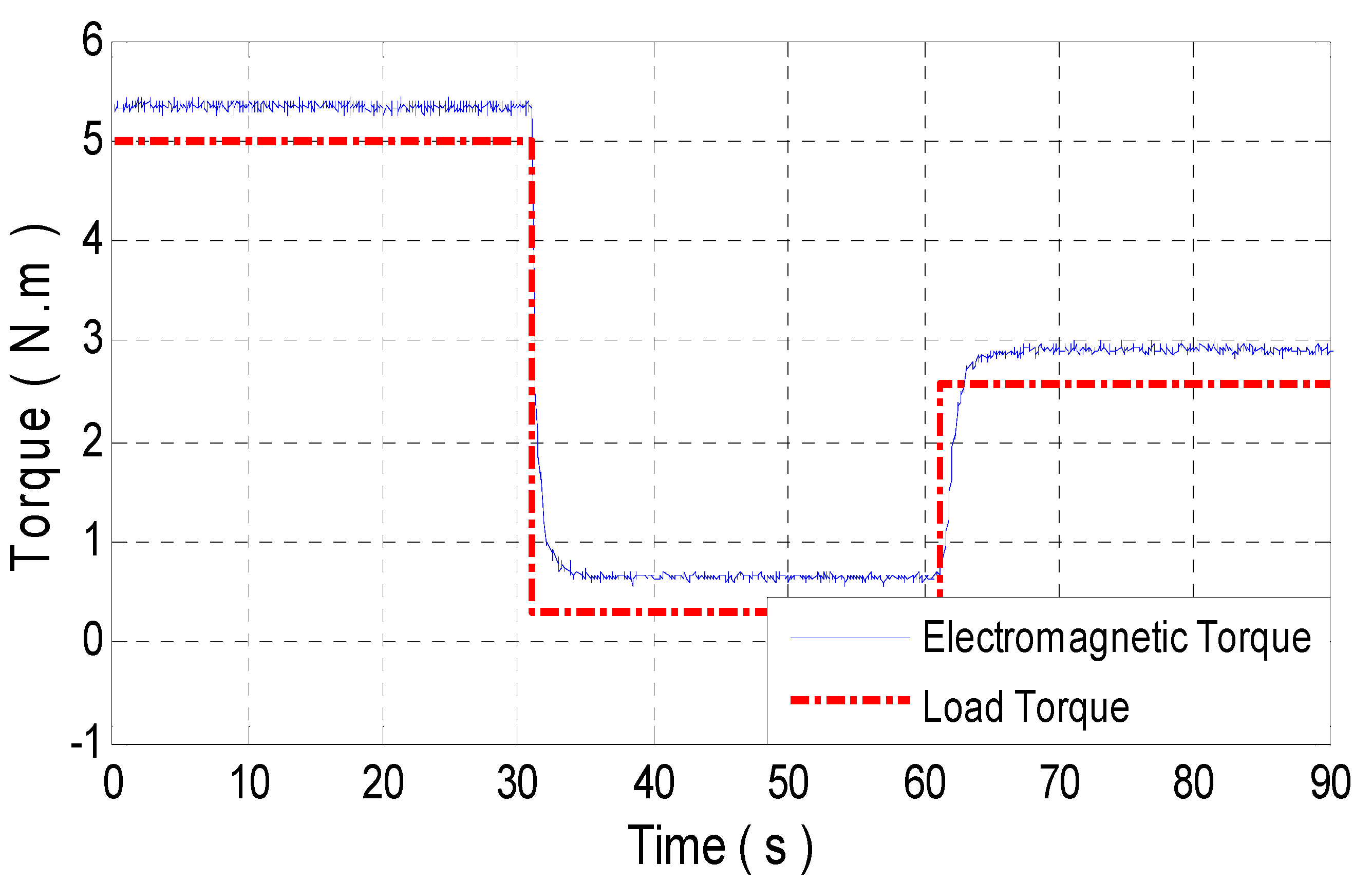
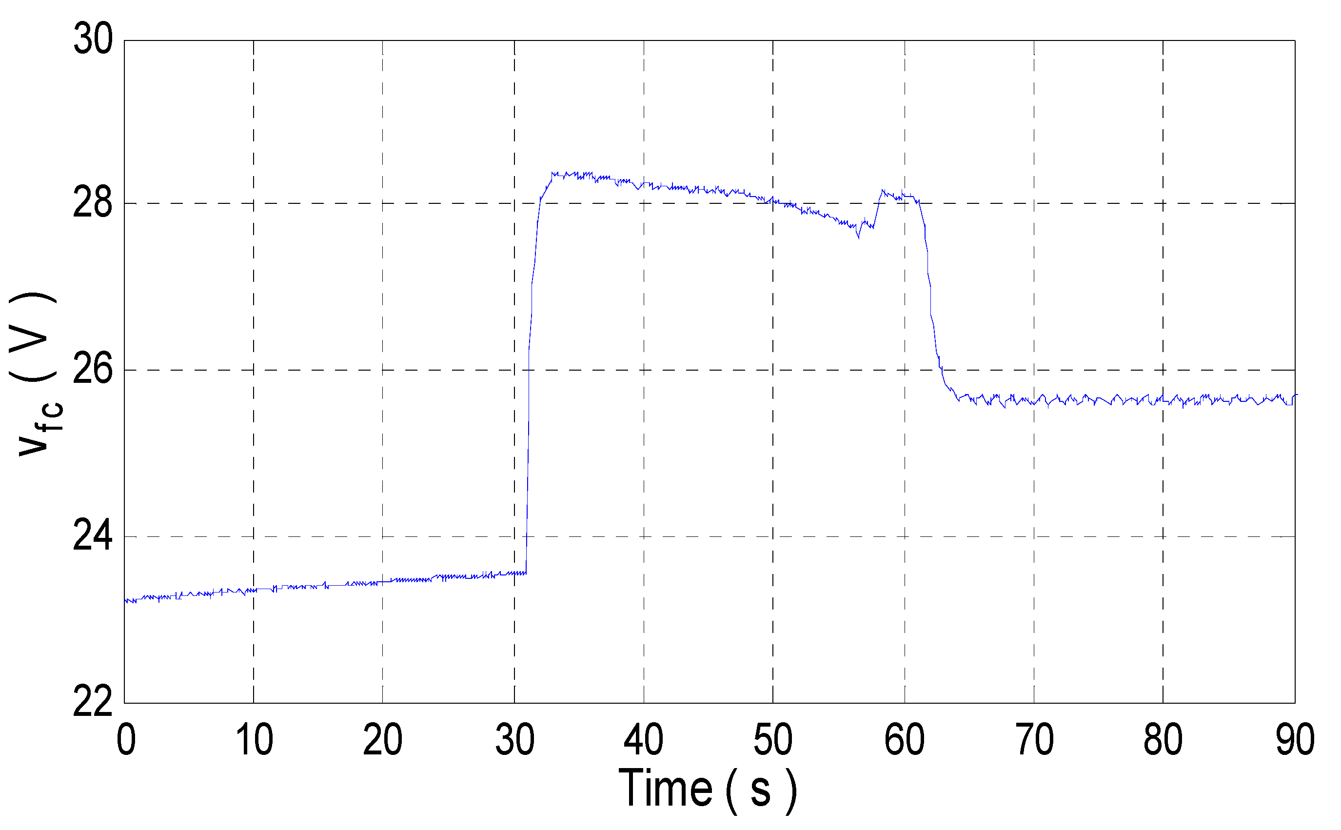
5. Experimental Results
- -
- Three metal hydride canisters from Heliocentris with storage capacities of 800 NL of hydrogen;
- -
- A Ballard Nexa 1200 fuel-cell module with its monitoring software;
- -
- A power supply from BK Precision.
- -
- A MicroLabBox-dSPACE DS1202 with Control Desk® software plugged into a Pentium 4 personal computer.
- -
- A salient-pole permanent-magnet synchronous motor;
- -
- A DC power supply;
- -
- A DC/AC converter;
- -
- A DC/DC converter;
- -
- A Hall-Effect current sensor;
- -
- A voltage sensor;
- -
- A digital scope;
- -
- A magnetic powder brake;
- -
- An encoder position sensor;
- -
- A torque sensor.
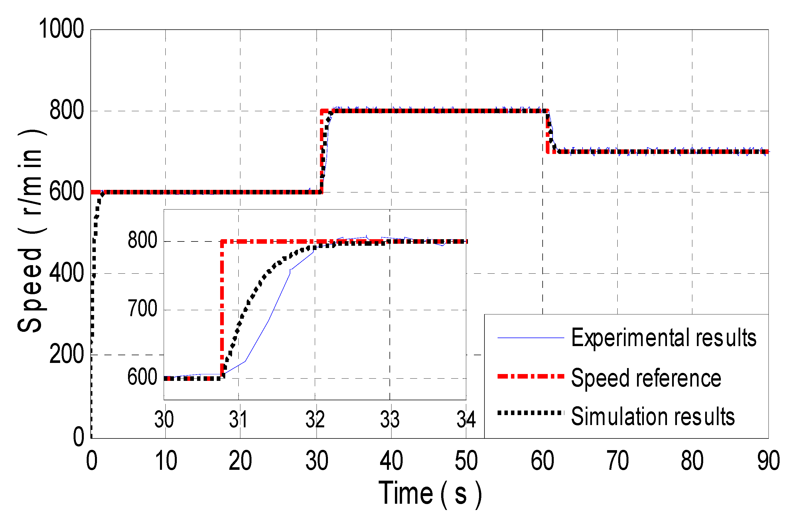
5.1. Speed Change
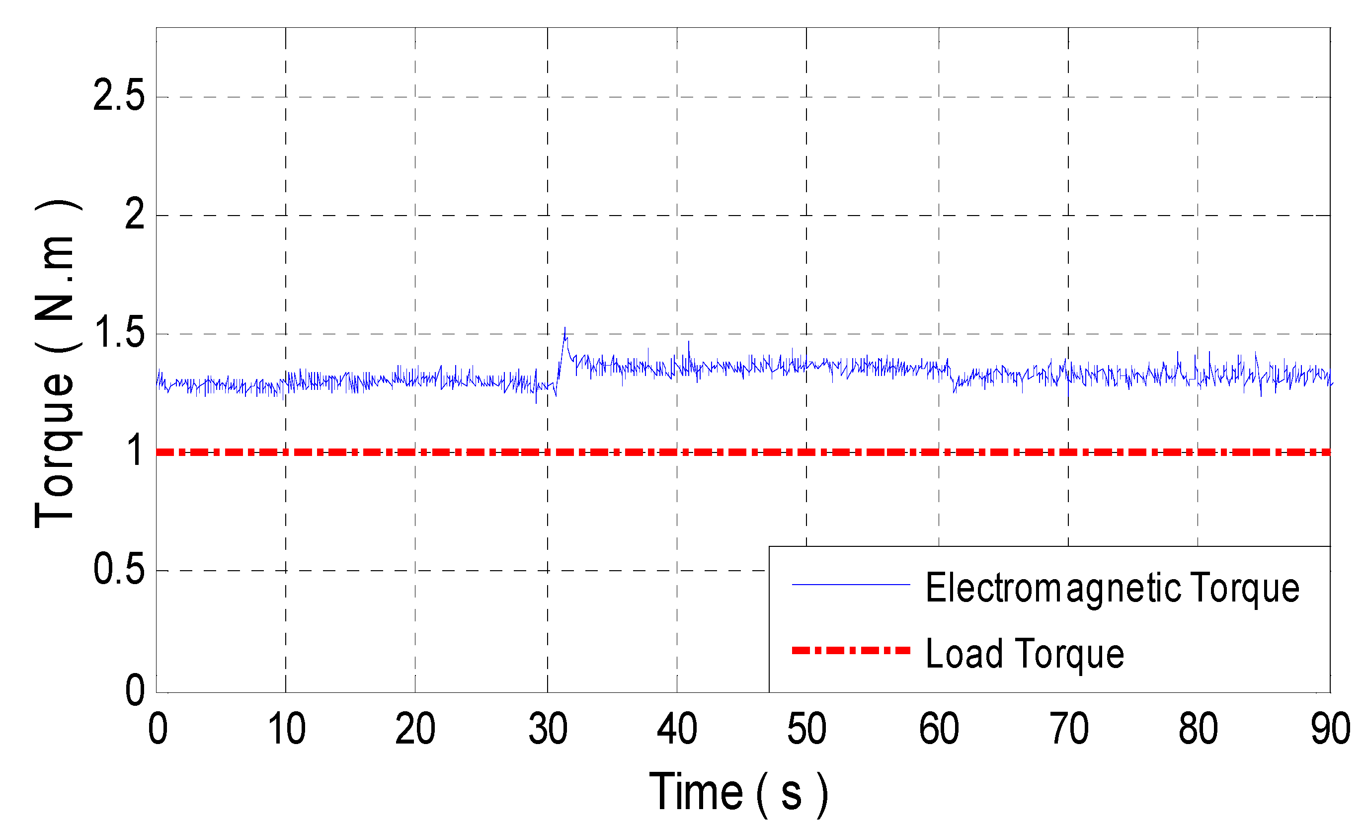
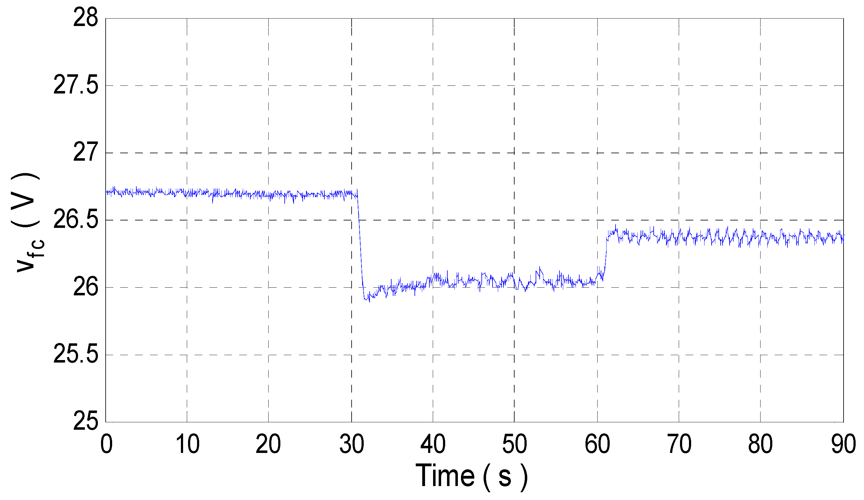
5.2. Torque Change
6. Conclusions
- -
- The perfect tracking of the vehicle speed to its reference;
- -
- The high stability of the closed-loop system;
- -
- The estimation of non-measurable parameters of the SP-PMSM such as f and J;
- -
- The estimation of the load torque Cr.
Author Contributions
Funding
Data Availability Statement
Conflicts of Interest
References
- Zhu, H.; Xiao, X.; Li, Y.-D. Stator flux control scheme for permanent magnet synchronous motor torque predictive control. Proc. Chin. Soc. Electr. Eng. 2010, 30, 86–90. [Google Scholar]
- Kazerooni, M.; Hamidifar, S.; Kar, N.C. Analytical modelling and parametric sensitivity analysis for the PMSM steady-state performance prediction. IET Electr. Power Appl. 2013, 7, 586–596. [Google Scholar] [CrossRef]
- Lin, F.J.; Hung, Y.C.; Tsai, M.T. Fault-tolerant control for six-phase PMSM drive system via intelligent complementary sliding-mode control using TSKFNN-AMF. IEEE Trans. Ind. Electron. 2013, 60, 5747–5762. [Google Scholar] [CrossRef]
- Gundogdu, T.; Zhu, Z.-Q.; Chan, C.C. Comparative Study of Permanent Magnet, Conventional, and Advanced Induction Machines for Traction Applications. World Electr. Veh. J. 2022, 13, 137. [Google Scholar] [CrossRef]
- Yang, T.; Chau, K.T.; Liu, W.; Ching, T.W.; Cao, L. Comparative Analysis and Design of Double-Rotor Stator-Permanent-Magnet Motors with Magnetic-Differential Application for Electric Vehicles. World Electr. Veh. J. 2022, 13, 199. [Google Scholar] [CrossRef]
- Yang, H.; Li, Y.; Lu, Q. Performance Simulation of Long-Stator Linear Synchronous Motor for High-Speed Maglev Train under Three-Phase Short-Circuit Fault. World Electr. Veh. J. 2022, 13, 216. [Google Scholar] [CrossRef]
- Sul, S.-K. Control of Electric Machine Drive Systems; Wiley-IEEE Books: Piscataway, NJ, USA, 2011. [Google Scholar]
- Xia, C.; Zhao, J.; Yan, Y.; Shi, T. A Novel Direct Torque Control of Matrix Converter-Fed PMSM Drives Using Duty Cycle Control for Torque Ripple Reduction. IEEE Trans. Ind. Electron. June 2014, 61, 2700–2713. [Google Scholar] [CrossRef]
- Du, B.; Wu, S.; Han, S.; Cui, S. Interturn fault diagnosis strategy for interior permanent-magnet synchronous motor of electric vehicles based on digital signal processor. IEEE Trans Ind. Electron. 2016, 63, 1694–1706. [Google Scholar] [CrossRef]
- Gaouzi, K.; El Fadil, H.; Idrissi, Z.E.; Lassioui, A. Digital implementation of model predictive control of an inverter for electric vehicles applications. Int. J. Modell. Identif. Control 2022, 40, 210–218. [Google Scholar] [CrossRef]
- Gaouzi, K.; El Fadil, H.; Belhaj, F.Z.; Idrissi, Z.E. Model Predictive Control of an Inverter for Electric Vehicles Applications. In Proceedings of the 2020 IEEE 2nd International Conference on Electronics, Control, Optimization and Computer Science (ICECOCS), Kenitra, Morocco, 2–3 December 2020; 2020; pp. 1–5. [Google Scholar] [CrossRef]
- El Fadil, H.; Idrissi, Z.E.; Intidam, A.; Rachid, A.; Koundi, M.; Bouanou, T. Nonlinear control and energy management of the hybrid fuel cell and battery power system. Int. J. Modell. Identif. Control 2021, 36, 89–103. [Google Scholar] [CrossRef]
- Putri, A.K.; Hombitzer, M.; Franck, D.; Hameyer, K. Comparison of the characteristics of cost-oriented designed high-speed low-power interior PMSM. IEEE Trans. Ind. Appl. 2017, 53, 5262–5271. [Google Scholar] [CrossRef]
- Singh, K.V.; Bansal, H.O.; Singh, D.A. Comprehensive review on hybrid electric vehicles: Architectures and components. J. Mod. Transp. 2019, 27, 77–107. [Google Scholar] [CrossRef] [Green Version]
- Chen, J.; Yao, W.; Ren, Y.; Wang, R.; Zhang, L.; Jiang, L. Nonlinear adaptive speed control of a permanent magnet synchronous motor: A perturbation estimation approach. Control Eng. Pr. 2019, 85, 163–175. [Google Scholar] [CrossRef]
- Vu, N.T.-T. A Nonlinear State Observer for Sensorless Speed Control of IPMSM. J. Control Autom. Electr. Syst. 2020, 31, 1087–1096. [Google Scholar] [CrossRef]
- Chen, C.-X.; Xie, Y.-X.; Lan, Y.-H. Backstepping control of speed sensorless permanent magnet synchronous motor based on slide model observer. Int. J. Autom. Comput. 2015, 12, 149–155. [Google Scholar] [CrossRef]
- Khlaief, A.; Boussak, M.; Chaari, A. A MRAS-based stator resistance and speed estimation for sensorless vector controlled IPMSM drive. Electr. Power Syst. Res. 2014, 108, 1–15. [Google Scholar] [CrossRef]
- Liu, X.-D.; Li, K.; Zhang, C.-H. Improved backstepping control with nonlinear disturbance observer for the speed control of permanent magnet synchronous motor. J. Electr. Eng. Technol. 2019, 14, 275–285. [Google Scholar] [CrossRef]
- Karabacak, M.; Eskikurt, H.I. Design, modelling and simulation of a new nonlinear and full adaptive backstepping speed tracking controller for uncertain PMSM. Appl. Math. Model. 2012, 36, 5199–5213. [Google Scholar] [CrossRef]
- Idrissi, Z.E.; El Fadil, H.; Giri, F. Nonlinear control of salient-pole PMSM for electric vehicles traction. In Proceedings of the IEEE Mediterranean Electrotechnical Conference, Marrakech, Morocco, 2–7 May 2018; pp. 231–236. [Google Scholar]
- Idrissi, Z.E.; El Fadil, H.; Belhaj, F.Z.; Oulcaid, M.; Gaouzi, K.; Lassioui, A. Non-linear Adaptive Observer for Salient-Pole PMSM for Hybrid Electric Vehicle Applications. In Proceedings of the 2020 International Conference on Electrical and Information Technologies (ICEIT), Rabat, Morocco, 4–7 March 2020; 2020; pp. 1–4. [Google Scholar] [CrossRef]
- Sun, X.; Yu, H.; Yu, J.; Liu, X. Design and implementation of a novel adaptive backstepping control scheme for a PMSM with unknown load torque. IET Electr. Power Appl. 2019, 13, 445–455. [Google Scholar] [CrossRef]
- El-Sousy, F.F.M.; El-Naggar, M.F.; Amin, M.; Abu-Siada, A.; Abuhasel, K.A. Robust Adaptive Neural-Network Backstepping Control Design for High-Speed Permanent-Magnet Synchronous Motor Drives: Theory and Experiments. IEEE Access 2019, 7, 99327–99348. [Google Scholar] [CrossRef]
- Zhang, J.; Wang, S.; Zhou, P.; Zhao, L.; Li, S. Novel prescribed performance-tangent barrier Lyapunov function for neural adaptive control of the chaotic PMSM system by backstepping. Int. J. Electr. Power Energy Syst. 2020, 121, 105991. [Google Scholar] [CrossRef]
- Krstiü, M.; Kanellakopoulos, I.; Kokotoviü, P.V. Nonlinear and Adaptive Control Design; John Wiley & Sons: Hoboken, NJ, USA, 1995. [Google Scholar]
- El Fadil, H.; Giri, F.; Haloua, M.; Ouadi, H. Nonlinear and Adaptive Control of Buck Power Converters. In Proceedings of the IEEE Conference on Decision and Control (CDC’03), Maui, HI, USA, 9–12 December 2003; pp. 4475–4480. [Google Scholar]
- Ammeh, L.; El Fadil, H.; Yahya, A.; Ouhaddach, K.; Giri, F.; Ahmed-Ali, T. A Nonlinear Backstepping Controller for Inverters used in Microgrids. In Proceedings of the 20th IFAC World Congress, Toulouse, France, 9–14 July 2017; pp. 7293–7298. [Google Scholar]
- Khalil, H.K. Nonlinear Control; Prentice Hall: Hoboken, NJ, USA, 2014. [Google Scholar]
- El Fadil, H.; Giri, F.; Guerrero, J.M.; Tahri, A. Modeling and Nonlinear Control of a Fuel Cell/Supercapacitor Hybrid Energy Storage System for Electric Vehicles. IEEE Trans. Veh. Technol. 2014, 63, 3011–3018. [Google Scholar] [CrossRef] [Green Version]


| Parameter | Value |
|---|---|
| Stator resistance Rs | 0.56 Ω |
| Number of pole pairs p | 3 |
| Rotation inertia J | 0.0021 kg.m2 |
| Flux of permanent magnet ψsf | 0.82 Wb |
| Inductance Ld | 0.048 H |
| Inductance Lq | 0.064 H |
| Viscous damping f | 0.0001 Nm/rd.s−1 |
| Rated voltage | 320 V |
| Rated power | 2 kW |
| Rated speed | 1800 r/mn |
| Parameter | Value |
|---|---|
| Output power | 1200 W |
| Output current | max. 55 A |
| Nominal voltage | 24 V |
| Output voltage | 0–32 V |
| Input voltage | 16–45 V |
| Operational temperature | −10–55 °C |
| Efficiency | >96% |
| Parameter | Value |
|---|---|
| Rated power | 1200 W |
| Rated current | 52 A |
| Rated voltage | 24 V |
| Output voltage | 20–36 V |
| Operational temperature | 5–40 °C |
| Parameter | Value |
|---|---|
| Output power | 2016 W |
| Output current | max. 42 A |
| Output voltage | 48 V |
| Input voltage | 24 V |
| Parameter | Value |
|---|---|
| Rated power | 1000 W |
| Rated current | 25.7 A |
| Rated voltage | 48 V |
| Rated speed | 1000 r/min |
| Rated torque | 10 N.m |
| Parameter | Value |
|---|---|
| Rated power | 2000 W |
| Rated voltage | 48 V |
| Continuous current | 60 A |
| Peak current | 150 A |
| Working frequency | 16.6 kHz |
| Parameter | Value |
|---|---|
| c1 | 20 |
| c2 | 2000 |
| c3 | 200 |
| γ1 | 0.003 |
| γ2 | 0.005 |
| γ3 | 0.007 |
Disclaimer/Publisher’s Note: The statements, opinions and data contained in all publications are solely those of the individual author(s) and contributor(s) and not of MDPI and/or the editor(s). MDPI and/or the editor(s) disclaim responsibility for any injury to people or property resulting from any ideas, methods, instructions or products referred to in the content. |
© 2023 by the authors. Licensee MDPI, Basel, Switzerland. This article is an open access article distributed under the terms and conditions of the Creative Commons Attribution (CC BY) license (https://creativecommons.org/licenses/by/4.0/).
Share and Cite
El Fakir, C.; El Idrissi, Z.; Lassioui, A.; Belhaj, F.Z.; Gaouzi, K.; El Fadil, H.; Rachid, A. Adaptive Nonlinear Control of Salient-Pole PMSM for Hybrid Electric Vehicle Applications: Theory and Experiments. World Electr. Veh. J. 2023, 14, 30. https://doi.org/10.3390/wevj14020030
El Fakir C, El Idrissi Z, Lassioui A, Belhaj FZ, Gaouzi K, El Fadil H, Rachid A. Adaptive Nonlinear Control of Salient-Pole PMSM for Hybrid Electric Vehicle Applications: Theory and Experiments. World Electric Vehicle Journal. 2023; 14(2):30. https://doi.org/10.3390/wevj14020030
Chicago/Turabian StyleEl Fakir, Chaimae, Zakariae El Idrissi, Abdellah Lassioui, Fatima Zahra Belhaj, Khawla Gaouzi, Hassan El Fadil, and Aziz Rachid. 2023. "Adaptive Nonlinear Control of Salient-Pole PMSM for Hybrid Electric Vehicle Applications: Theory and Experiments" World Electric Vehicle Journal 14, no. 2: 30. https://doi.org/10.3390/wevj14020030