Cost Minimization for Charging Electric Bus Fleets

Abstract

Recent attention for reduced carbon emissions has pushed transit authorities to adopt battery electric buses (BEBs). One challenge experienced by BEB users is extended charge times, which create logistical challenges and may force BEBs to charge when energy is more expensive. Furthermore, BEB charging leads to high power demands, which can significantly increase monthly power costs and may push the electrical infrastructure beyond its present capacity, requiring expensive upgrades. This work presents a novel method for minimizing the monthly cost of BEB charging while meeting bus route constraints. This method extends previous work by incorporating a more novel cost model, effects from uncontrolled loads, differences between daytime and overnight charging, and variable rate charging. A graph-based network-flow framework, represented by a mixed-integer linear program, encodes the charging action space, physical bus constraints, and battery state of the charge dynamics. The results for three scenarios are considered: uncontested charging, which uses equal numbers of buses and chargers; contested charging, which has more buses than chargers; and variable charge rates. Among other findings, we show that BEBs can be added to the fleet without raising the peak power demand for only the cost of the energy, suggesting that conversion to electrified transit is possible without upgrading power delivery infrastructure.

1. Introduction

Recent calls for a reduced carbon footprint have led transit authorities to adopt battery electric buses (BEBs). Replacing diesel and CNG buses with BEBs reduces environmental impact [1], as BEBs provide zero vehicle emissions and can access renewable energy sources [2,3].

Charging BEBs draws power from the electrical infrastructure. The combined effect of BEB charging with other necessary loads can exceed the capacity of local distribution circuits [4,5,6], leading to expensive infrastructure upgrades. Power providers pass the cost of upgrades on to customers. Thus, the benefits of large-scale electrified bussing seem appealing at first but are only practical if infrastructural upgrades can be deferred or avoided altogether.

One approach to deferring or avoiding upgrades is to intentionally manage when and at what rates buses should charge. An optimal charge plan must account for a number of physical constraints and operational realities. For example, buses must exceed a minimum charge level while adhering to route schedules, batteries must have sufficient time to charge, and buses must share a limited number of chargers. The focus of this work is to find an optimal charge schedule which meets these requirements and minimizes the cost of electricity and grid impacts in the presence of other uncontrolled loads. This problem is referred to hereafter as the “charge problem”.

Previous work has done much to further state of the art in this regard with solutions ranging from heuristic approaches and linear programs to battery exchanges (see Section 2 for details). The contributions our paper offers, which we have not observed in the current literature, is the combination of (1) differences in night and day charging, (2) the ability to vary charge rates, (3) incorporating non-BEB grid activity into the optimization scheme, and (4) the use of a real-world rate schedule which encompasses both time-of-use energy rates and demand fees to reduce the instantaneous load on the grid.

Without these elements, a charge schedule may not fully utilize the available charging resources to reduce the monthly cost of energy. For example, Rocky Mountain Power may charge upwards of USD 15.00 per kW for the largest use of instantaneous power over a 15 min window, which may account for over a third of the monthly power expenses. Additionally, Rocky Mountain Power may also charge close to double for energy used during on-peak hours. While previous work has addressed time-of-use tariffs [7] and instantaneous power demand [8], we have not seen these elements together, and minimizing using Rocky Mountain Power’s rate schedule provides a clear way of integrating the two.

Another example where our work addresses unsolved issues lies on the use of night/day charge parameters. In the Utah Transit Authority station in Salt Lake City, Utah, buses are able to charge on a limited number of fast overhead chargers during the day, and an unlimited number of slower chargers at night. By breaking the problem into day and night segments, we encode these differences into the optimization framework. For a comprehensive list of contributions, please see Section 2.3.

The remainder of this paper is organized as follows: Section 2 describes prior related work, and Section 3 outlines a graph-based framework for modeling the environment, including buses, routes, chargers, and uncontrolled loads. Section 4 incorporates the problem constraints involving battery charge dynamics, and Section 5 extends the the graph framework to account for differences between day and night operations. Section 6 translates the rate schedule used for billing into an objective function. Finally, Section 7 and Section 8 present results and describe future work, respectively.

2. Literature Review

This section summarizes prior work related to the charge problem and includes discussion on battery charging and managing runtime costs. The final subsection discusses the contributions of this paper and how they relate to prior methods.

2.1. Battery Charging

Recharging BEBs is more time consuming than refueling diesel and CNG buses [9]. A diesel or CNG engine can refuel in several minutes, but an electric bus may require several hours to charge, making the extended charge time a primary concern for BEB conversion.

To circumvent long refuel times, refs. [10,11] propose an approach which replaces batteries when the state of charge is low. The exchange would replace the current battery with one that is fully charged and recharge the spent batteries afterward. Exchanging batteries reduces the down time but is non-trivial because battery swapping requires specialized tools and/or automation.

Another alternative is to inductively charge buses while they are in motion. Dynamic charging simplifies logistics because it eliminates the need for stationary charging. Both [12] and [13] propose methods that inductively charge BEBs using specialized hardware in the road. Furthermore, dynamic charging is supported by various planning algorithms, such as [14,15,16].

Recharging BEBs at a station requires only the development of an intelligent charge schedule. Following a charge schedule requires minimal modifications to the charging infrastructure and utilizes existing charging ports in the BEBs with no need for additional tools or automation. Algorithms for planning use foreknowledge of the runtime environment and battery dynamics to identify when and to which buses chargers should connect. Planning algorithms discussed in this review are considered on a scale from “reactive” to “global”, where reactive methods respond to stimuli at the present, and global techniques assume complete knowledge about the operating environment to form a plan.

Because reactive planning generally focuses on present circumstances, it requires minimal knowledge of the operational environment, making reactive planning extremely versatile and scalable. Methods of this type are both computationally efficient and adapt to many use cases. One such example is illustrated in [17], which splits the total power draw between the grid and an external battery to regulate the instantaneous load. The authors of [18] give another approach which uses a Markov Decision Process to instantaneously make decisions.

Reactive algorithms can be enhanced by encoding details for future events to improve decision making. If only event details within a finite horizon are used, the algorithm becomes a hybrid, containing features of both reactive and global techniques. For example, [19] describes a technique for optimizing a charging schedule out to a scheduling horizon. Changing the horizon adjusts both the scope and computational complexity of the solution. In stochastic environments, a smaller window is beneficial, as charge schedules must be frequently recomputed, whereas in more stable circumstances, longer windows can yield improved performance. Multi-agent collaboration has also been studied in the present context [20] and includes methods for load distribution both temporally and spatially [21,22]

Global algorithms include all information from the beginning to the end. Because global algorithms assume complete foreknowledge of future events, they provide globally optimal plans and achieve the highest performance. Global algorithms can encompass a number of scenarios, including hardware that is either distributed [23] or collocated, although many times, a distributed scenario is not feasible due to the added cost or scarce charger locations.

The authors in [9,24,25,26,27] present techniques that formulate constrained optimization problems which provide solutions in terms of binary charge decisions for each bus at each timestep while constraining the power use to comply with contractual obligations. Work from [7] even minimizes the total cost of power using a time of day pricing schedule. The authors in [28] take a somewhat different approach by encoding the bus constraints in a graph and solving for an optimal solution using a network-flow approach. The discrete nature of the graph-based approach allows [28] to model a non-linear charge dynamic based on the constant current constant voltage model. The methods given by [24,25,28,29] address the problem of scheduling buses while meeting the constraints for power use; however, this technique could be extended by considering non-BEB activity on the grid. In particular, results from [29] will be used as a comparison for this class of algorithms later in this paper.

The authors of [30] provide a technique which accounts for grid activity by assuming that the external grid behavior is known a priori and incorporating its effects into a cost function. Other methods such as [31] similarly rely on a priori data but focus on price management in the presence of an ever-changing electrical market. However, in locations such as Salt Lake City, Utah, the electrical market is heavily regulated, and the price of energy has a fixed cost given by the power provider so that market-driven strategies are less applicable.

2.2. Cost Optimization

In addition to physical constraints such as bus routes and charging dynamics, this paper focuses on minimizing the cost associated with charging and minimizes fees assessed for on- and off-peak energy use, on- and off-peak power demand, and facilities power charges [32]. Prior work dealt with charge costs in various ways. The authors in [33] propose a method to forecast power use. The work conducted by [8] proposes a method which reduces the demand charge by using power forecasts to plan charge times [33]. When forecasting is not possible, both refs. [17,34] propose methods that decrease the power demand by observing the load and drawing additional power from on-site battery packs. Additionally, ref. [24] minimize over on/off-peak energy as part of their work.

2.3. Contributions

This paper develops a novel charge schedule planning framework, which extends the planner proposed by [28] to include multi-rate charging, uncontrolled loads, night/day charging, and the rate schedule given in [32]. Our method formulates the bus charge problem as a mixed-integer linear program (MILP) and is unique because the objective function is the cost for the transit authority (bus fleet operator) and includes charges for on-peak and off-peak energy use, on-peak and off-peak power demand, and facilities demand. The proposed framework handles contention for charging resources in a globally optimal manner, which guarantees charger availability even when chargers are scarce.

Prior work also made assumptions for night time charge behavior. Our work eliminates the need for such by including both day and night charging in the charge schedule. The modeling of night and day charging also includes their respective operational constraints, such as charge rates, bus availability, and the number of available chargers.

Our work also seeks to understand how the variable rate, as compared to single rate charging, affects the cost optimality and contributes a more accurate representation of battery charging dynamics.

Furthermore, because the proposed method includes operational characteristics, such as the number of buses, the number of chargers, the battery capacity, and various route metadata in the constraints, it complements prior work which determined such parameters [35,36].

The final contribution is recognizing that our framework is a tool that enables the prediction of monthly costs for transit authorities and infrastructure demand for power providers. Optimized charging schedules reduce the power demand and extend the lifetime of the electrical infrastructure.

3. Graph-Based Problem Formulation

This section formulates the charge problem as an optimization problem where the variables are defined in a graph. The first subsection describes the intuition behind this graph-based approach, and the second develops a series of equality and inequality constraints resulting in a mixed-integer linear program (MILP).

3.1. Graph Formulation

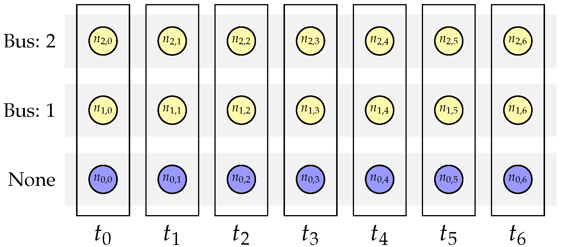
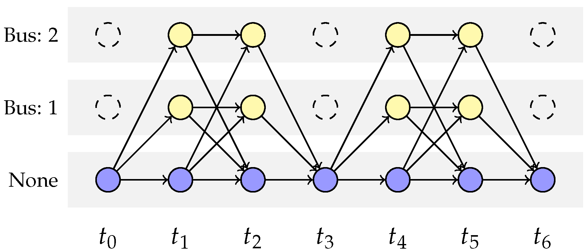
A solution to the bus charge problem is a schedule of actions for charging equipment. A schedule states both when and to which bus a charger should connect, suggesting a model with two dimensions. The first dimension represents time and is given discretely in a left to right fashion. The second dimension encodes the charger state and extends vertically as shown in Figure 1. The charger may be in one of several possible states. For example, it may be connected to one of the N buses, or it may be unconnected, giving a total of $N+1$ different states. This (time, state) 2-D representation is encoded as a rectangular grid of nodes. Node $n_{i,j}$ represents the charger in the ith state during the jth time index (see Figure 1). For example, $n_{1,0}$ from Figure 1 represents a state where a charger is connected to Bus 1 at $t_0$.

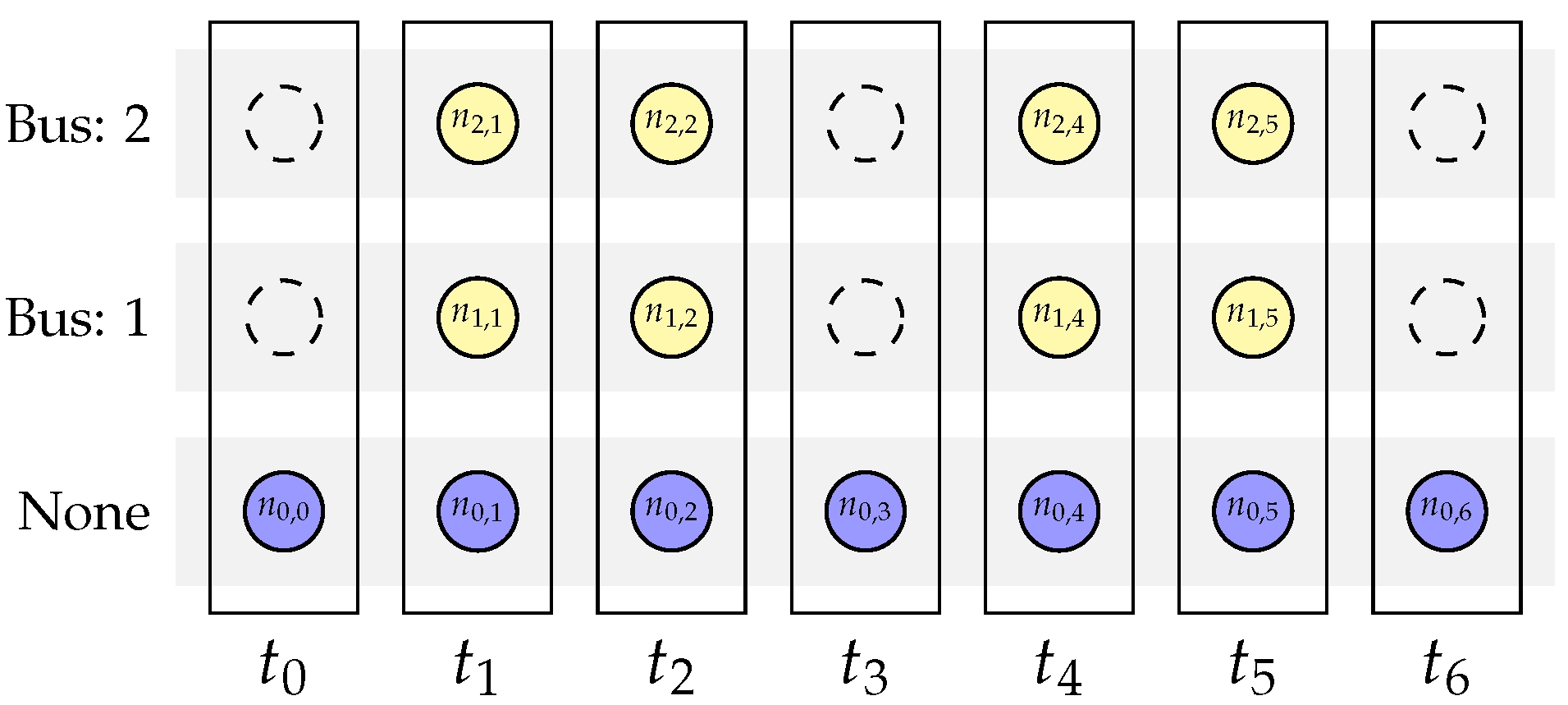
We want the grid of nodes to encode the times at which each bus is at the station and available for charging. Therefore, let a node be present in the grid when the corresponding bus can connect to a charger, and delete nodes from the grid when a bus is away from the station. Consider the two-bus scenario from Figure 1, where buses 1 and 2 are away from the station at $t_0$, $t_3$, and $t_6$. The schedule is encoded by removing $n_{1,0}$, $n_{2,0}$, $n_{1,3}$, $n_{2,3}$, $n_{1,6}$, and $n_{2,6}$ to reflect the grid shown in Figure 2.

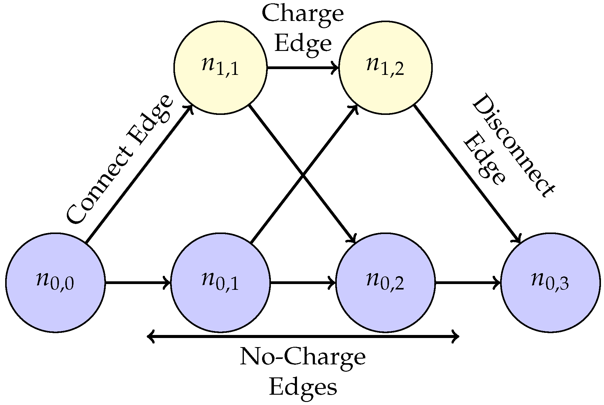
The state of a charger at any time is represented by existing in a particular node. Changes in charger state over time are represented by the transitions from a node to multiple possible next nodes. These transitions are called edges (see Figure 3) and represent four possible decisions: connect to a bus, charge a bus, remain idle, or disconnect from a bus. Edges are associated with actions, and that action is determined by the nodes on either end. Consider the edge from $n_{0,0}$ to $n_{0,1}$ in Figure 4. This edge represents a no-charge decision because the nodes on both ends represent the disconnected charge state at times $t_0$ and $t_1$. Chargers cannot charge while disconnected, so the edge decision is no charge. Similarly, the edge between $n_{1,1}$ and $n_{1,2}$ indicates a decision to charge, as both $n_{1,1}$ and $n_{1,2}$ represent states where a charger is connected at times $t_1$ and $t_2$. Both to-charge and no-charge decisions are represented by horizontal transitions in the graph and only reflect the passing of time, as no changes to the physical hardware are made.

Conversely, diagonal transitions imply physical hardware changes because they represent decisions where chargers connect to or disconnect from a bus. One such example from Figure 4 includes the edge from $n_{0,0}$ to $n_{1,1}$. The state represented by $n_{0,0}$ is disconnected. This edge represents an interval where a charger is disconnected at $t_0$ and connected at $t_1$, implying a ‘to-connect’ decision. The same logic applies in reverse for the edge between $n_{1,2}$ and $n_{0,3}$. Hence, the bus charge problem can be described in terms of nodes and edges (i.e., a graph) where nodes represent bus availability for charging and edges encode all possible charge decisions.

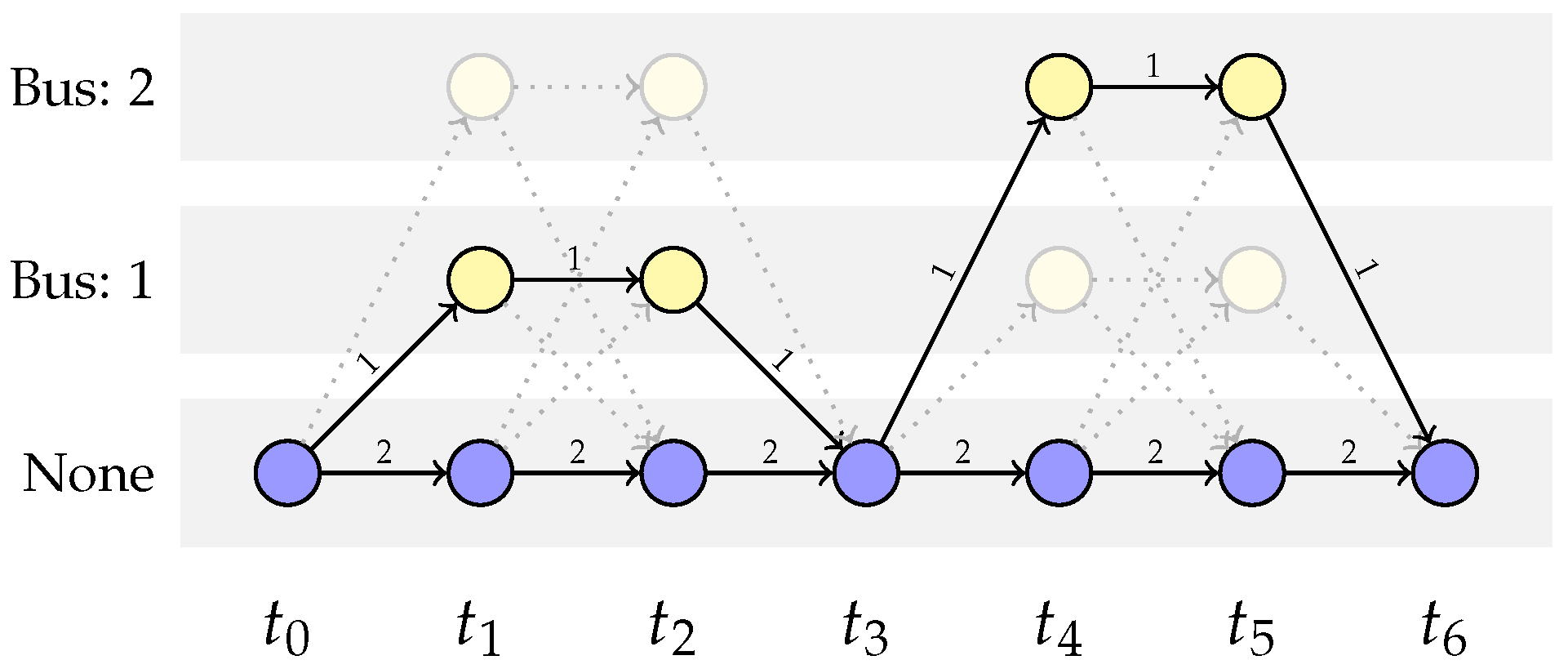
A charge schedule can be thought of as a list of charge decisions that govern charge behavior. Because decisions are represented by edges in the graph, a schedule is also represented by a sequence of connected edges that form a path through the graph. If an edge is selected, or active, it is considered part of the path. Active and inactive edges are represented edge weights equal to 1 and 0, respectively.

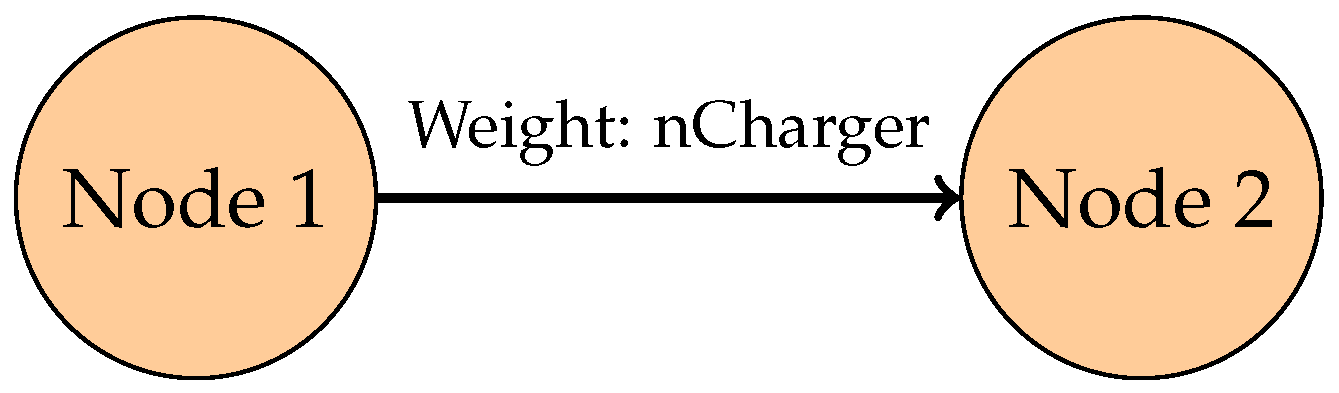
A graph with binary edge weights can only represent a plan for one charger. This representation can be expanded to represent an arbitrary number of chargers by using integer valued weights, where each weight gives the number of chargers in the transition.

Consider a three-charger scenario using the graph in Figure 5. A solution where one charger is connected to Bus 1 from $t_1$ to $t_2$ and to Bus 2 from $t_4$ to $t_5$ would be expressed by assigning unit weights to the appropriate connect, charge, and disconnect edges. The second charger remains idle as illustrated by the active edges along the bottom row of charger states (see Figure 6).

In summary, the graph encodes bus availability with nodes, decisions with edges, and schedules with edge weights. Solving the bus charge problem becomes a matter of finding the optimal set of edge weights, where optimal is meant to denote the most cost-effective charge plan.

3.2. Graph Constraints

Finding the optimal charge schedule can be expressed as an optimization problem, where the graph is used to derive equality and inequality constraints for a mixed-integer linear program (MILP)

$$\begin{array}{cc}\hfill & \underset{\mathbf{y}}{\min }{\mathbf{r}}^T\mathbf{y}\mathrm{subject}\mathrm{to}\hfill \\ \hfill & F\mathbf{y}=\mathbf{f},Q\mathbf{y}\le \mathbf{q},\hfill \end{array}$$

(1)

where the equality and inequality constraints are encoded in F, $\mathbf{f}$, Q and $\mathbf{q}$. The variable $\mathbf{y}$ is a vector containing the elements of the solution and has the form

$${\mathbf{y}}^T=\left[\begin{array}{c}{\mathbf{x}}^T{\mathbf{d}}^T{\mathbf{g}}^T{\mathbf{e}}^T{\mathbf{p}}^T{\widehat{p}}_{\mathrm{off}-\mathrm{peak}}{\widehat{p}}_{\mathrm{on}-\mathrm{peak}}\end{array}\right],$$

(2)

where $\mathbf{x},\mathbf{d},\mathbf{g},\mathbf{e},\mathbf{p},{\widehat{p}}_{\mathrm{off}-\mathrm{peak}}$, and ${\widehat{p}}_{\mathrm{on}-\mathrm{peak}}$ represent the edge weights of the graph, the bus state of charge, the changes in the state of charge, the energy used, the average power at each timestep, the maximum off-peak power, and the maximum on-peak power, respectively. Each variable will be defined as unknown elements in a mixed-integer linear program and will receive greater attention throughout this paper.

This subsection formulates two sets of constraints. The first represents the graph structure, enforces the conservation of chargers, and defines the number of chargers through a set of net-flow constraints. The second prevents the charger from thrashing between connected/disconnected states and enforces one-bus/one-charger connectivity by enforcing what we call “group flow” constraints.

3.2.1. Net-Flow Constraints

Network flow constraints are expressed in matrix–vector form as

$$\begin{array}{c}\hfill A\mathbf{x}={\mathbf{c}}_f,\end{array}$$

(3)

where A is the graph incidence matrix, $\mathbf{x}$ is the $n_E\times 1$ vector of edge weights and corresponds to $\mathbf{x}$ in Equation (2), and ${\mathbf{c}}_f$ is $n_N\times 1$ and equals the difference between incoming and outgoing edge weights, or net-flow. The parameter $n_E$ is the number of edges, and $n_N$ is the number of nodes.

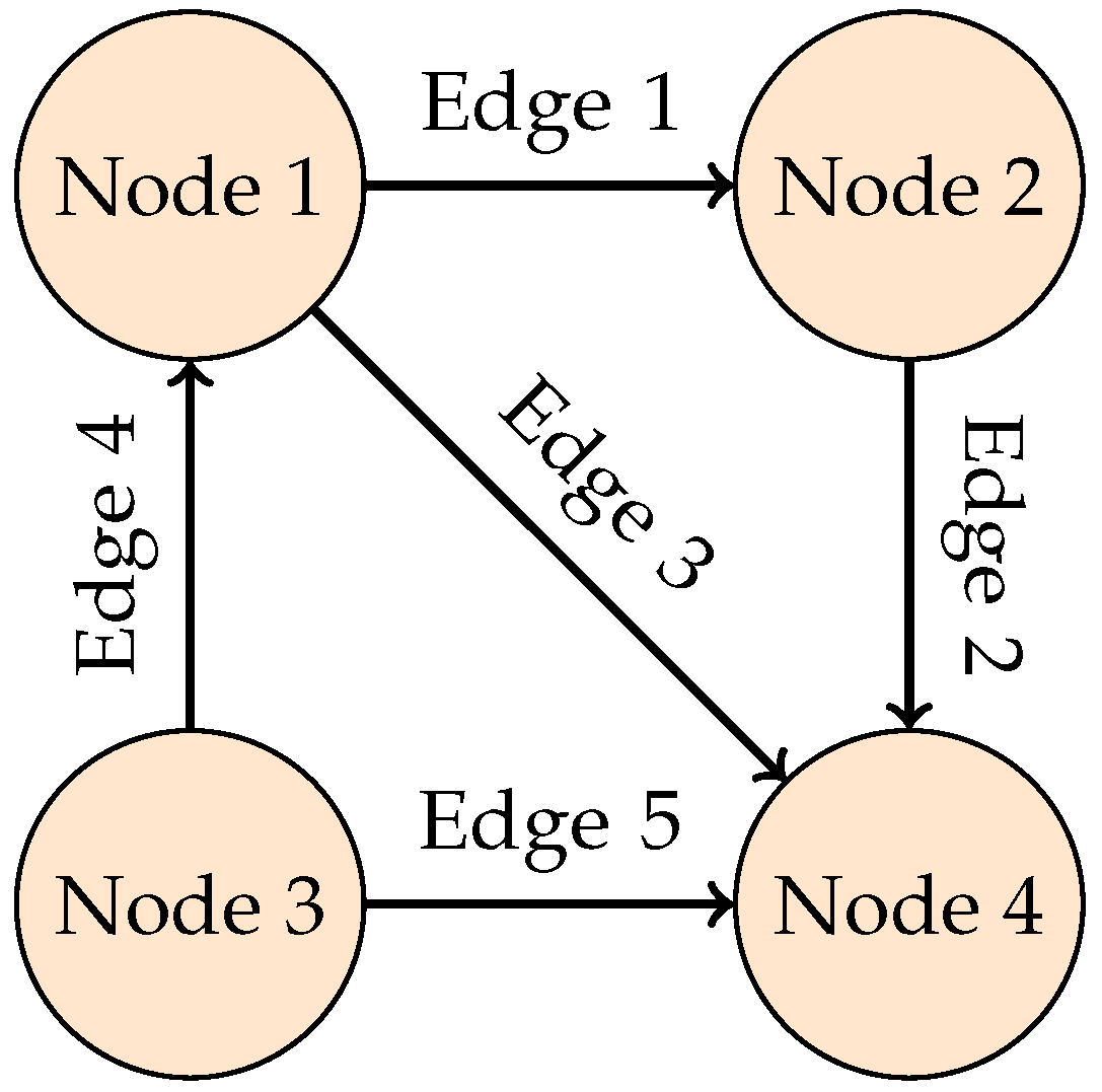
An incidence matrix organizes relationships between nodes and edges by describing which edges leave and enter which nodes. The matrix A is an $n_N\times n_E$ matrix and expresses incoming connections between the $i^{\mathrm{th}}$ node and $j^{\mathrm{th}}$ edge by $A_{i,j}=1$. Similarly, outgoing connections are given by $A_{i,j}=-1$, and no connection with $A_{i,j}=0$. For example, the graph in Figure 7 is represented as follows.

$$\begin{array}{c}\hfill \left[\begin{array}{ccccc}-1& 0& -1& 1& 0\\ 1& -1& 0& 0& 0\\ 0& 0& 0& -1& -1\\ 0& 1& 1& 0& 1\end{array}\right].\end{array}$$

(4)

The difference between the number of chargers entering and leaving, or the net-flow, can be expressed in terms of A as seen in Equation (3). Because the number of chargers does not change, the number of chargers entering and leaving a node must be equal. This is expressed in linear form as $a_i^{T}x=0$, where $a_i$ is the ith row of A. The only exceptions occur at source and sink nodes.

A source node represents the beginning state for all chargers. Because edges originate here, there are no incoming edges, and the net-flow will be minus the number of chargers. This is described in linear form as $a_i^{T}x=-n_C$, where $n_C$ is the number of chargers.

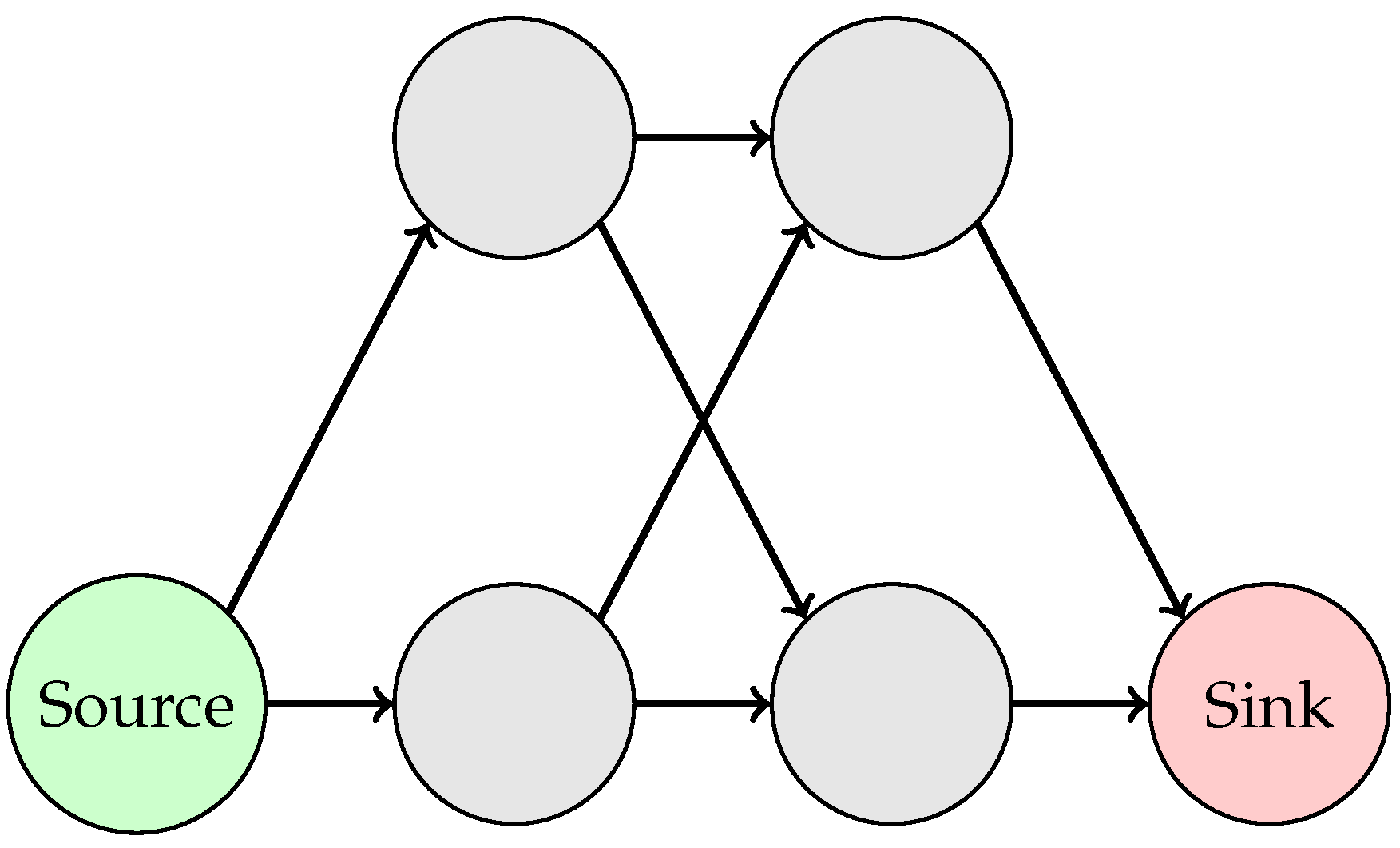
Sink nodes represent the final state, where all edges terminate (see Figure 8). Because sinks have no outgoing edges, they maintain a positive net-flow equal to the number of chargers and is expressed by $a_i^T=n_C$.

Therefore, the flow constraints require the elements of ${\mathbf{c}}_f$ to be equal to zero for all non-source and non-sink nodes as seen in Equation (5):

$$\begin{array}{c}\hfill Ax={\left[\begin{array}{c}0\dots -n_C\dots 0n_C\dots 0\end{array}\right]}^T.\end{array}$$

(5)

Equation (5) can be formulated in terms of $\mathbf{y}$ by appropriately zero-padding A such that

$$\begin{array}{cc}\hfill c_f& =\left[\begin{array}{cc}A& 0\end{array}\right]\mathbf{y}\hfill \\ \hfill & =\tilde{A}\mathbf{y}.\hfill \end{array}$$

(6)

3.2.2. Group Flow Constraints

Another flow type, known as group flow, can be used to regulate the number of chargers entering a set of nodes. This is desired for two reasons. First, it prevents chargers from connecting multiple times during an interval when a bus is available for charging, and it limits the number of chargers connecting to a bus to be one at most.

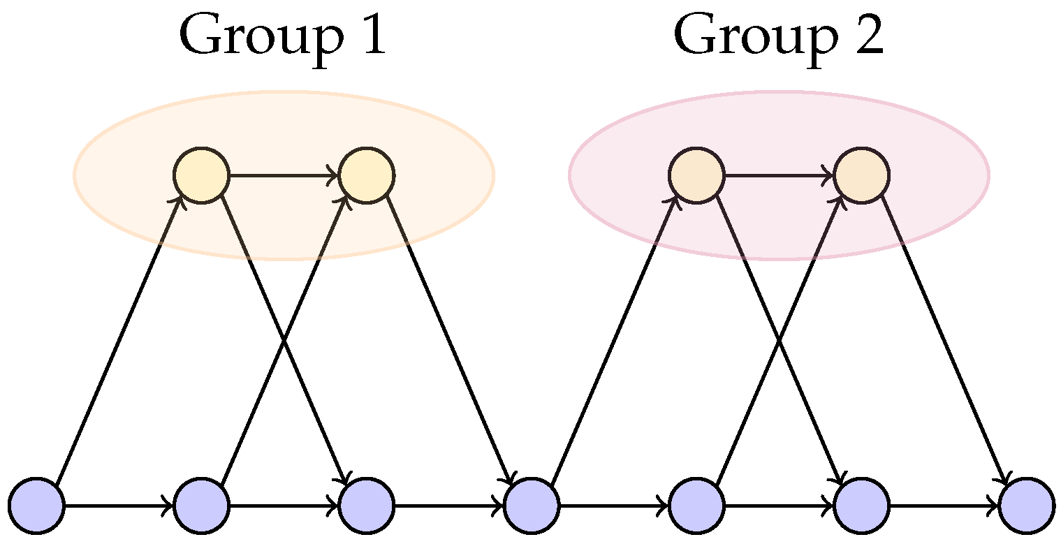
Define a charge group as the set of all nodes for a given bus corresponding to one station visit as shown in Figure 9. The group flow is the number of chargers that enter a group and is represented as the sum of all incoming edge weights (see Figure 10).

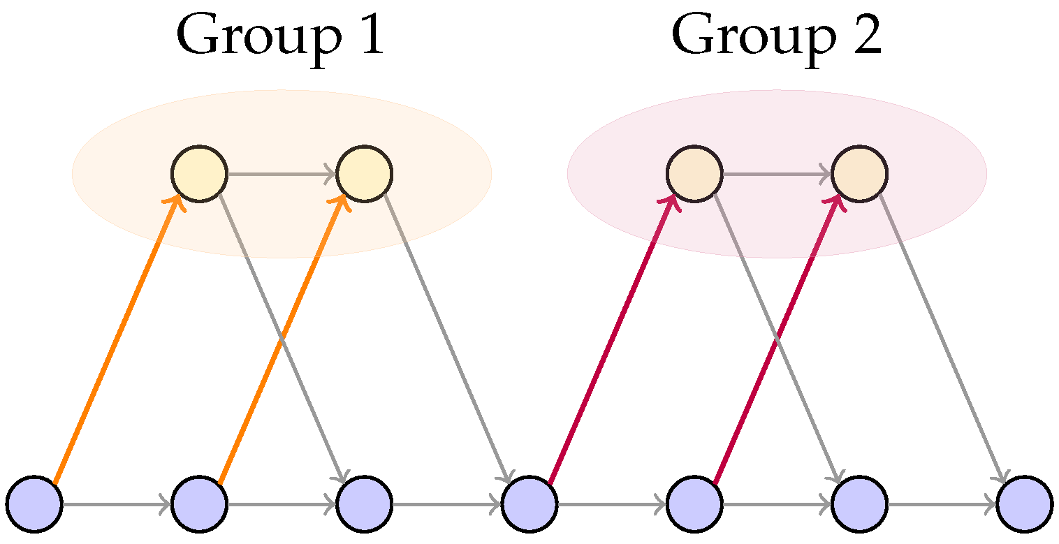
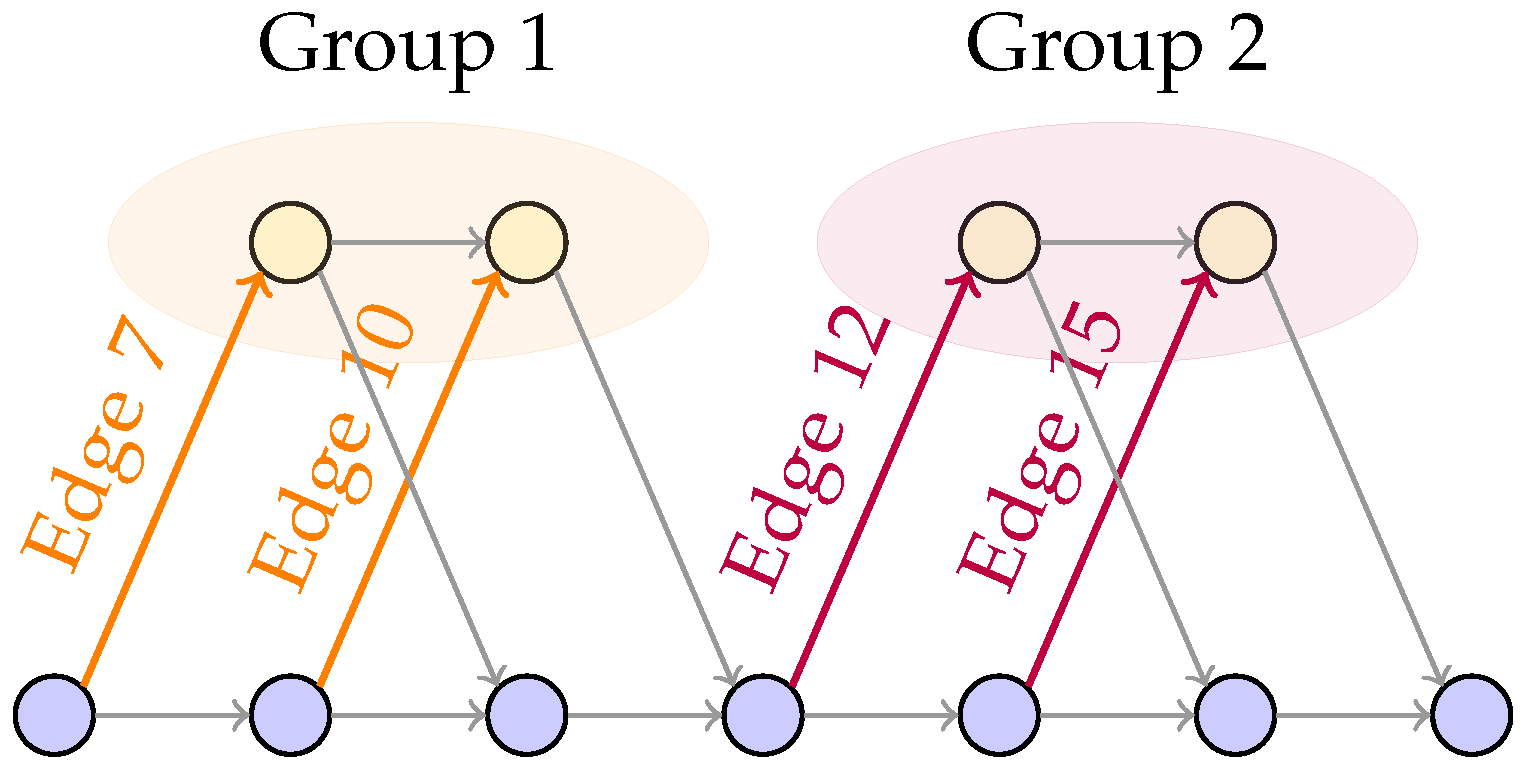
Denote the $n_G\times n_E$ group incidence matrix as B, where $n_G$ is the number of groups and $B_{i,j}$ is 1 if the jth edge enters the ith group and 0 otherwise. For example, the group incidence matrix corresponding to the graph in Figure 11 contains 1 in the 7th and 10th columns for Group 1, and the 12th and 15th columns for group 2 as given in Equation (7) so that

$$\begin{array}{c}\hfill B=\left[\begin{array}{c}0000001001000000\\ 0000000000010010\end{array}\right].\end{array}$$

(7)

Let $\mathbf{x}$ be the edge weights as before and ${\mathbf{c}}_g$ be an $n_G\times 1$ vector, where the ith element gives the group flow for group i. The group flow is then computed as

$$\begin{array}{c}\hfill B\mathbf{x}={\mathbf{c}}_g.\end{array}$$

(8)

Note that group flow is required to be one at most to avoid connection thrashing. This is expressed by the inequality given in Equation (9):

$$\begin{array}{c}\hfill Bx\le \mathbf{1}.\end{array}$$

(9)

Similarly to (6), Equation (9) can also be expressed in terms of $\mathbf{y}$ with appropriate zero padding as

$$\begin{array}{cc}\hfill \left[\begin{array}{cc}B& 0\end{array}\right]\mathbf{y}& =\tilde{B}\mathbf{y},\hfill \end{array}$$

(10)

so that

$$\tilde{B}\mathbf{y}\le \mathbf{1}.$$

(11)

3.3. Section Summary

In summary, the bus charge problem can be formulated as a graph with nodes and edges, where charge plans are encoded as a path with unit edge weights. The charge problem aims to find a feasible path which minimizes the cost of power. Feasibility is defined through a set of net-flow and group-flow constraints. Net-flow constraints are encoded through an adjacency matrix and enforce both the conservation and total number of chargers. The group-flow constraints prevent connection thrashing and limit to one the number of simultaneous charger-to-bus connections.

4. Battery State of Charge

The battery state of charge (SOC) plays a central role in the bus charge problem because a charge plan must ensure that all buses are adequately charged throughout the day. Therefore, the charge decisions must account for buses with lower SOC values and higher discharge rates along their respective routes. This section presents a formulation for tracking the expected SOC for each bus and imposes constraints on the optimization framework so that the SOC for each bus is guaranteed to exceed a minimum threshold throughout the day. Additionally, this method is run over a 24 h period, and the results are extrapolated to anticipate the cost over a month. Therefore, additional constraints are given so that buses begin and end each day with the same SOC.

A SOC thresholding constraint requires that battery charge levels be modeled. The kth SOC for bus i is denoted $d_{i,k}$, where k is the node index. The node indices used here are not directly tied to specific timesteps. For example, $d_{i,k+1}$ represents the bus SOC at the node in the graph following the node where $d_{i,k}$ is the SOC as seen in Figure 12. The set of all $d_{i,k}$ can be organized as the vector $\mathbf{d}$ from Equation (2).

Because no charging is performed while on route, $d_{i,k}$ will assume its lowest value when buses enter the charge station. Let $d_{i,k+1}$ be the charge level for bus i as it enters the charge station, and ${\delta }_i$ represent the power discharged while on route. The entrance SOC can be expressed as

$$\begin{array}{c}\hfill d_{i,k+1}=d_{i,k}-{\delta }_i,\end{array}$$

(12)

where $d_{i,k}$ is the previous departure SOC for bus i. Consider the example in Figure 13, where buses 1 and 2 leave the station at $t_2$ and enter at $t_4$. The corresponding change in SOC is given as $d_{1,2}=d_{1,1}-{\delta }_1$ and $d_{2,2}=d_{2,1}-{\delta }_2$ for buses 1 and 2, respectively.

The constraints from Equation (12) can be expressed in linear standard form as

$$\left[\begin{array}{cc}-1& 1\end{array}\right]\left[\begin{array}{c}{d}_{i,k}\\ d_{i,k+1}\end{array}\right]={\delta }_i.$$

(13)

Equation (13) can be expressed in terms of $\mathbf{y}$ with appropriate zero padding and expanded to account for the decrease in SOC for all buses outside the station. The expanded constraint is given as

$$\begin{array}{cc}\hfill \left[\begin{array}{cccccc}0& \dots & -1_{d_{i,k}}& 0& \dots & 1_{d_{i,k+1}}\end{array}\right]\mathbf{y}& ={\mathbf{d}}_{\delta }\hfill \\ \hfill D_{\delta }\mathbf{y}& ={\mathbf{d}}_{\delta },\hfill \end{array}$$

(14)

where $-1_{d_{i,k}}$ and $1_{d_{i,k+1}}$ represent $-1$ and 1 in locations corresponding to $d_{i,k}$ and $d_{i,k+1}$, respectively. Similar notation will be used throughout this paper as a means to imply a corresponding index for other variables.

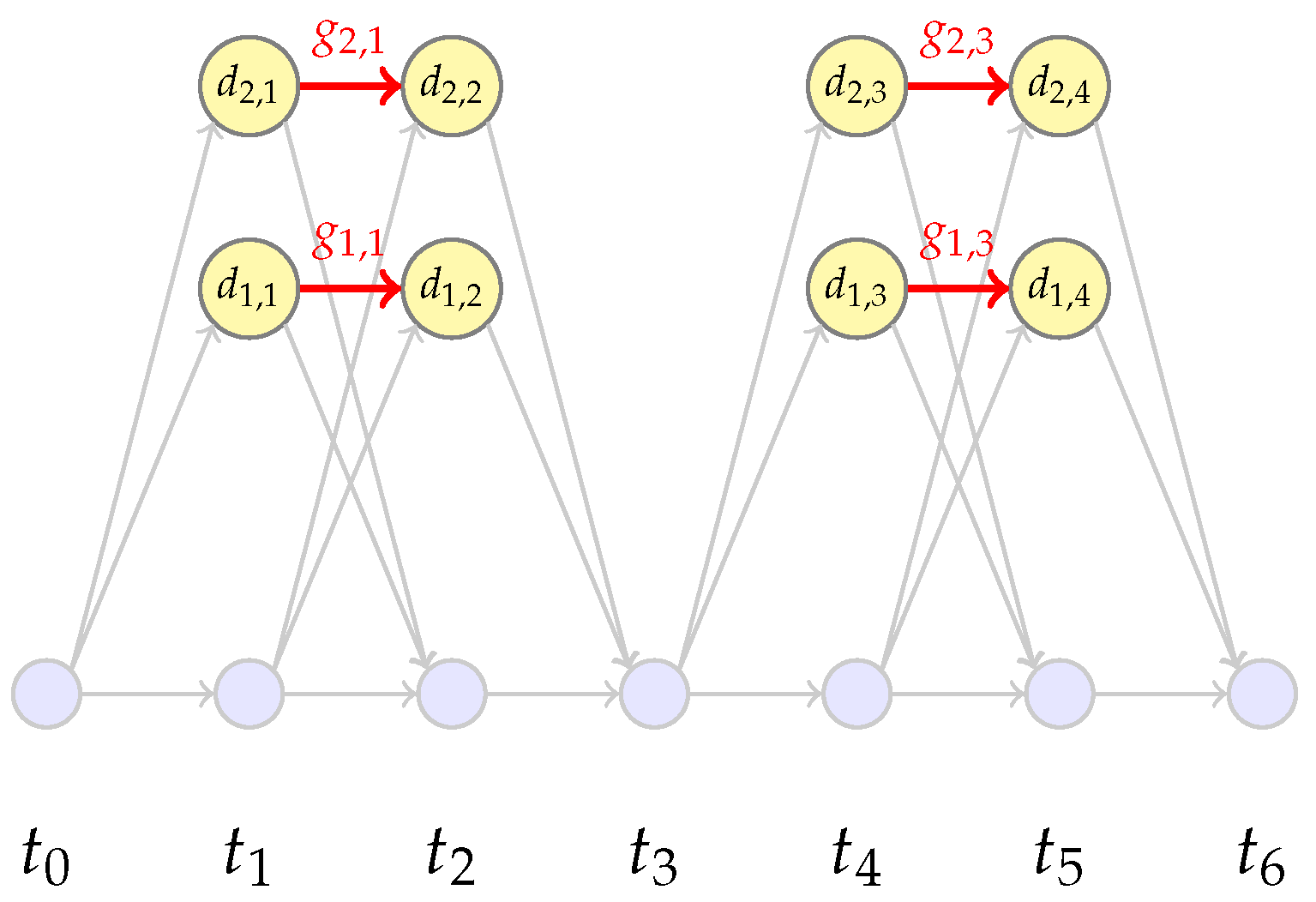
Time periods between entrance and exit nodes represent the time spent in the charge station and have the potential to charge the battery. An edge over which charging occurs is referred to as $x_{i,k}$, where k gives the index of the edge’s outgoing node, and i refers to the bus. When a charger occupies $x_{i,k}$, the resulting increase, or gain, in battery charge is denoted as $g_{i,k}$, where i and k mirror the edge indices (see Figure 12).

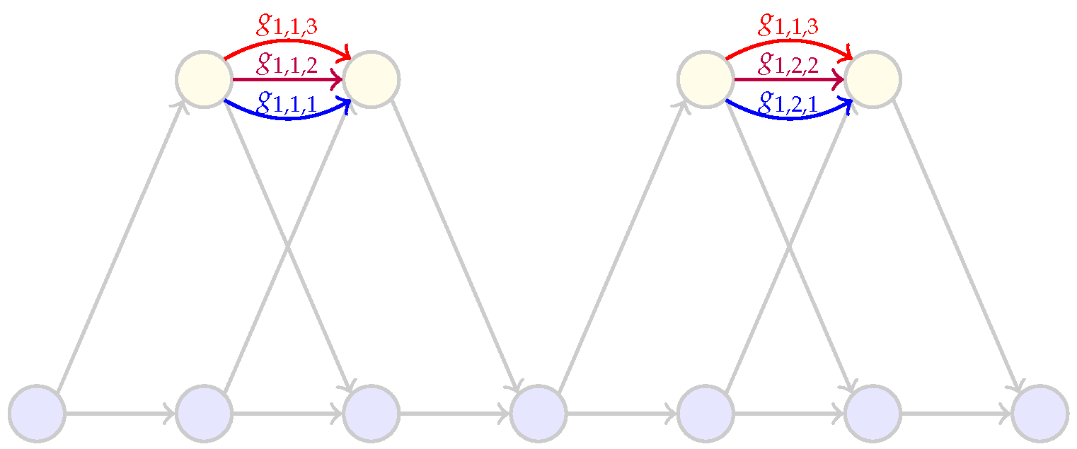
The value for $g_{i,k}$ is computed using a single charge rate. Multiple charge rates can be encoded by connecting bus nodes with multiple edges, denoted $x_{i,k,l}$, where each edge has a distinct charge rate and gain denoted $g_{i,k,l}$ (see Figure 14). Having multiple charge rates gives the option for fast charging when necessary and slow charging when possible to preserve battery health and decrease the electrical load [37].

The rate is selected by setting $x_{i,k,l}=1$. All gains associated with unselected rates are set to zero. Gains that correspond to selected rates are computed using the constant current constant voltage (CCCV) model as derived in [28], which gives:

$$\begin{array}{c}\hfill d_{i,k+1}={\overline{a}}_l{d}_{i,k}-{\overline{b}}_{l}M,\end{array}$$

(15)

where ${\overline{a}}_l$$\sim (0,1]$ depends on the charge rate and is experimentally determined, M is the battery capacity in kWh, and ${\overline{b}}_l={\overline{a}}_l-1$. Equation (15) is used to show that

$$\begin{array}{cc}\hfill d_{i,k+1}& ={\overline{a}}_l{d}_{i,k}-{\overline{b}}_{l}M\hfill \\ \hfill d_{i,k+1}-d_{i,k}& ={\overline{a}}_l{d}_{i,k}-{\overline{b}}_{l}M-d_{i,k},\hfill \end{array}$$

(16)

but the gain is equal to the difference in $d_{i,k+1}$ and $d_{i,k}$ such that $g_{i,k,l}=d_{i,k+1}-d_{i,k}$. So

$$\begin{array}{cc}\hfill g_{i,k,l}& ={\overline{a}}_l{d}_{i,k}-{\overline{b}}_{l}M-d_{i,k}\hfill \\ \hfill g_{i,k,l}& =({\overline{a}}_l-1)d_{i,k}-\overline{b_l}M.\hfill \end{array}$$

(17)

Therefore,

$$\{\begin{array}{cc}{g}_{i,k,l}=d_{i,k}({\overline{a}}_l-1)-{\overline{b}}_{l}M\hfill & x_{i,k,l}=1\hfill \\ g_{i,k,l}=0\hfill & x_{i,k,l}=0\hfill \end{array}.$$

(18)

The conditions given in Equation (18) can be rewritten as

$$\begin{gathered} \{\begin{array}{cc}\begin{array}{c}{g}_{i,k,l}\le d_{i,k}({\overline{a}}_l-1)-{\overline{b}}_{l}M\hfill \\ g_{i,k,l}\ge d_{i,k}({\overline{a}}_l-1)-{\overline{b}}_{l}M\hfill \end{array}\hfill & \hfill x_{i,k,l}=1\\ \begin{array}{c}{g}_{i,k,l}\le 0\hfill \\ g_{i,k,l}\ge 0\hfill \end{array}\hfill & x_{i,k,l}=0\hfill \end{array} \\ \Rightarrow \begin{array}{c}{g}_{i,k,l}\le d_{i,k}({\overline{a}}_l-1)-\overline{b}M-M(1-x_{i,k,l})\hfill \\ g_{i,k,l}\ge d_{i,k}({\overline{a}}_l-1)-\overline{b}M\hfill \\ g_{i,k,l}\le 0+M{x}_{i,k,l}\hfill \\ g_{i,k,l}\ge 0,\hfill \end{array} \end{gathered}$$

(19)

where M is the battery capacity. The results of Equation (19) obtain a switching effect. When $x_{i,k,l}=1$, Equation (19) becomes

$$\begin{gathered} \begin{array}{cc}{g}_{i,k,l}\le d_{i,k}({\overline{a}}_l-1)-{\overline{b}}_{l}M\hfill & \\ \hfill g_{i,k,l}\ge d_{i,k}({\overline{a}}_l-1)-{\overline{b}}_{l}M& \end{array}\left\}\mathrm{Active} \\ \begin{array}{cc}{g}_{i,k,l}\le M\hfill & \\ g_{i,k,l}\ge 0\hfill & \end{array}\right\}\mathrm{Inactive}. \end{gathered}$$

(20)

The active constraints imply equality for $g_{i,k,l}$ = $({\overline{a}}_l-1)d_{i,k}-\overline{b_l}M$. The inactive constraints imply that $g_{i,k,l}$ is greater than zero and less than the battery capacity, which are trivially satisfied. When $x_{i,k,l}=0$, Equation (19) becomes

$$\begin{gathered} \begin{array}{cc}{g}_{i,k,l}\le d_{i,k}({\overline{a}}_l-1)-{\overline{b}}_{l}M-M\hfill & \\ g_{i,k,l}\ge d_{i,k}({\overline{a}}_l-1)-{\overline{b}}_{l}M\hfill & \end{array}\left\}\mathrm{Inactive} \\ \begin{array}{cc}{g}_{i,k,l}\le 0\hfill & \\ g_{i,k,l}\ge 0\hfill & \end{array}\right\}\mathrm{Active}, \end{gathered}$$

(21)

where the inactive constraints are again trivially satisfied, and the active constraints imply equality for $g_{i,k,l}=0$.

Equation (19) can be expressed in standard form as

$$\begin{array}{cc}\hfill -g_{i,k,l}+d_{i,k}({\overline{a}}_l-1)+x_{i,k,l}& \le M(\overline{b_l}+1)\hfill \\ \hfill g_{i,k,l}-d_{i,k}({\overline{a}}_l-1)& \le -\overline{b_l}M\hfill \\ \hfill g_{i,k,l}-M{x}_{i,k,l}& \le 0\hfill \\ \hfill -g_{i,k,l}& \le 0,\hfill \end{array}$$

(22)

and in matrix form as

$$\left[\begin{array}{ccc}-1& {\overline{a}}_l-1& 1\\ 1& 1-{\overline{a}}_1& 0\\ 1& 0& -M\\ -1& 0& 0\end{array}\right]\left[\begin{array}{c}{g}_{i,k,l}\\ d_{i,k}\\ x_{i,k,l}\end{array}\right]\le \left[\begin{array}{c}M({\overline{b}}_l+1)\\ -{\overline{b}}_{l}M\\ 0\\ 0\end{array}\right].$$

(23)

Equation (23) can be expanded to include constraints for all $g_{i,k,l}$. Because each value for $g_{i,k,l}$, $d_{i,k}$, and $x_{i,k,l}$ is an element of $\mathbf{y}$, the constraints from Equation (23) can be written as

$$G\mathbf{y}\le {\mathbf{b}}_g.$$

(24)

The value of $d_{i,k}$ can be expressed as

$$d_{i,k+1}=d_{i,k}+\sum _l{g}_{i,k,l},$$

(25)

or

$$d_{i,k+1}-d_{i,k}-\sum _l{g}_{i,k,l}=0,$$

(26)

because a non-zero element of $g_{i,k,l}$ is only present for one corresponding l. This relationship is described in terms of an equality constraint such that

$$\left[\begin{array}{cccc}1& -1& \dots & -1\end{array}\right]\left[\begin{array}{c}{d}_{i,k+1}\\ d_{i,k}\\ g_{i,k,1}\\ \dots \\ g_{i,k,l}\end{array}\right]=0.$$

(27)

Equation (27) can be appropriately zero padded to give

$$\left[\begin{array}{cccc}{1}_{d_{i,k+1}}& -1_{d_{i,k}}& \dots & -1_{g_{i,k,l}}\end{array}\right]\mathbf{y}=0.$$

(28)

and expanded to define the values for all $d_{i,k}\ni k>0$ as

$$D_d\mathbf{y}=\mathbf{0}.$$

(29)

The values for $d_{i,0}$ are defined with initial SOC conditions with additional equality constraints denoted as ${\mathbf{d}}_0$ such that

$$\left[\begin{array}{ccccc}{1}_{d_{1,0}}& 0& 0& \dots & 0\\ 0& \dots & 1_{d_{2,0}}& 0& 0\\ ⋮& & ⋮& & ⋮\\ 0& 0& 0& \dots & 1_{d_{i,0}}\end{array}\right]\mathbf{y}={\mathbf{d}}_0,$$

(30)

or

$$D_0\mathbf{y}={\mathbf{d}}_0.$$

(31)

Once all values for $d_{i,k}$ are computed, they must be constrained to remain above threshold $\tau$. The SOC thresholding constraint can be expressed as an inequality constraint such that

$$\begin{array}{cc}\hfill & d_{i,k}\ge \tau \hfill \\ \hfill \Rightarrow & -d_{i,k}\le -\tau \hfill \\ \hfill \Rightarrow & \left[\begin{array}{ccccc}0& \dots & -1_{d_{i,k}}& \dots & 0\end{array}\right]\mathbf{y}\le -\tau .\hfill \end{array}$$

(32)

Equation (32) can be expanded to a matrix $D_{\tau }$, where each $d_{i,k}$ contains a corresponding constraint row such that

$$\begin{array}{cc}\hfill D_{\tau }\mathbf{y}& \le -\tau \mathbf{1}\hfill \\ \hfill & \le {\mathbf{d}}_{\tau }.\hfill \end{array}$$

(33)

In summary, the minimum SOC for all feasible charge plans must exceed a given threshold. SOC values are computed while the bus is in the charge station. SOC values are updated when a bus enters by subtracting the discharged energy from the previous SOC estimate. SOC values are updated for in-station periods by adding the charge gains as given in Equation (25). Gains are computed using a switching constraint, which sets them to zero when not charging; otherwise, they follow the CCCV model as set forth in Equation (17). Initial SOC values are handled with the equality constraint given in Equation (31), and the SOC is constrained to remain above the threshold $\tau$ in Equation (33). All constraints for d can be concatenated such that

$$\left[\begin{array}{c}{D}_0\\ D_{\delta }\\ D_d\end{array}\right]\mathbf{y}=\left[\begin{array}{c}{\mathbf{d}}_0\\ {\mathbf{d}}_{\delta }\\ \mathbf{0}\end{array}\right],\left[\begin{array}{c}{D}_g\\ D_{\tau }\end{array}\right]\mathbf{y}\le \left[\begin{array}{c}{\mathbf{d}}_g\\ {\mathbf{d}}_{\tau }\end{array}\right],$$

(34)

and expressed as

$$D_{\mathrm{eq}}\mathbf{y}={\mathbf{d}}_{\mathrm{eq}},D_{\mathrm{ineq}}\mathbf{y}\le {\mathbf{d}}_{\mathrm{ineq}}.$$

(35)

5. Multi-Graph Additions

An additional contribution this work offers is the expansion to the joint optimization of both night and day charging in a single optimization problem. Day and night operations differ in two aspects: number of chargers and bus availability. During the day, the buses can charge only at the charge station. The number of chargers in the station are limited, causing contention between buses. At night, each bus docks in a holding stall with one charger per stall, eliminating charger contention. Furthermore, nighttime charging is slow compared to daytime charging. Our model uses different rates for day and night charging.

Bus availability also changes because buses do not leave their stalls at night. This simplifies the charge problem because buses are always available for charging.

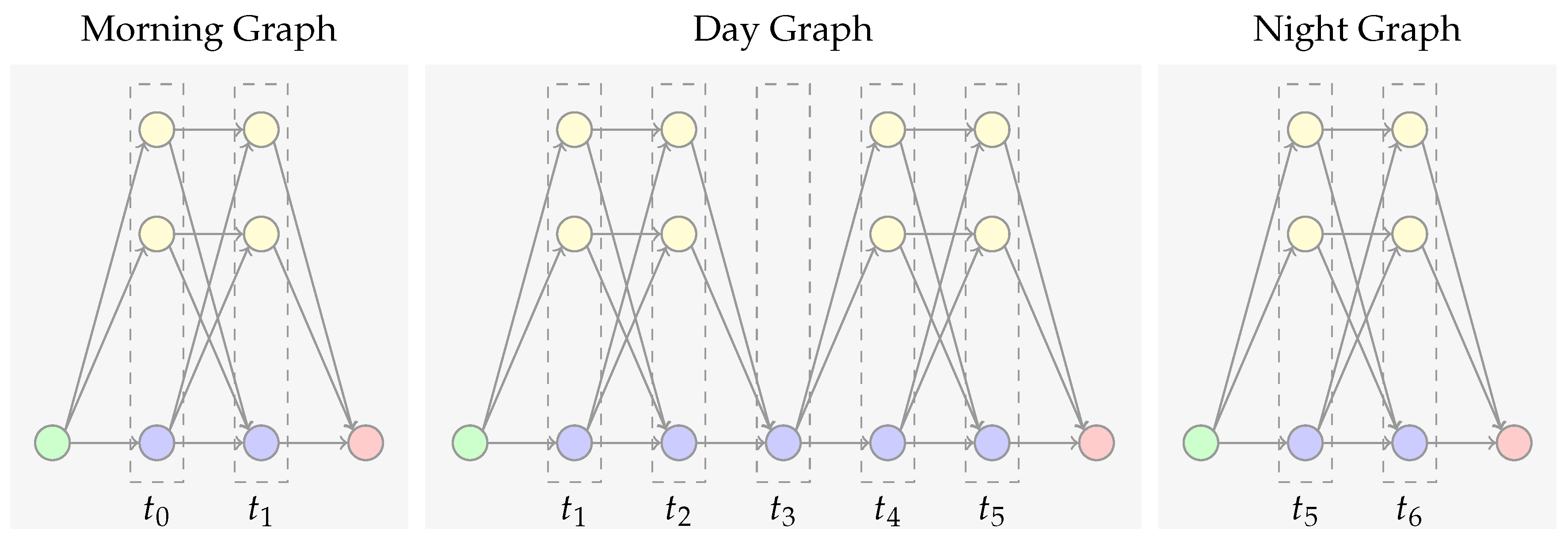
Equation (5) in Section 3.2.1 describes the net-flow constraints which constrain the number of chargers in the source and sink nodes. Because the number of chargers are different from night to day, a separate graph is used at each transition as shown in Figure 15.

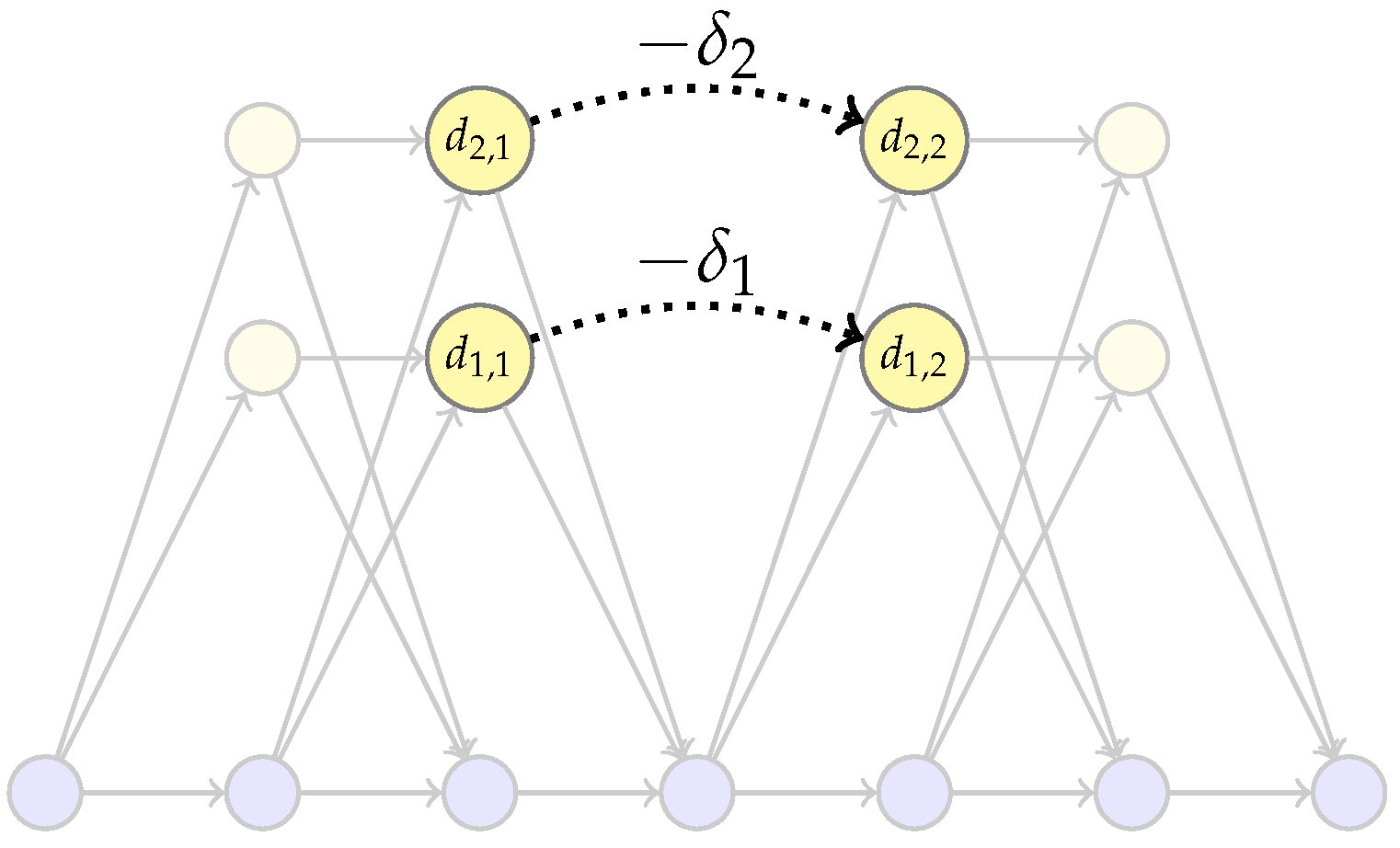
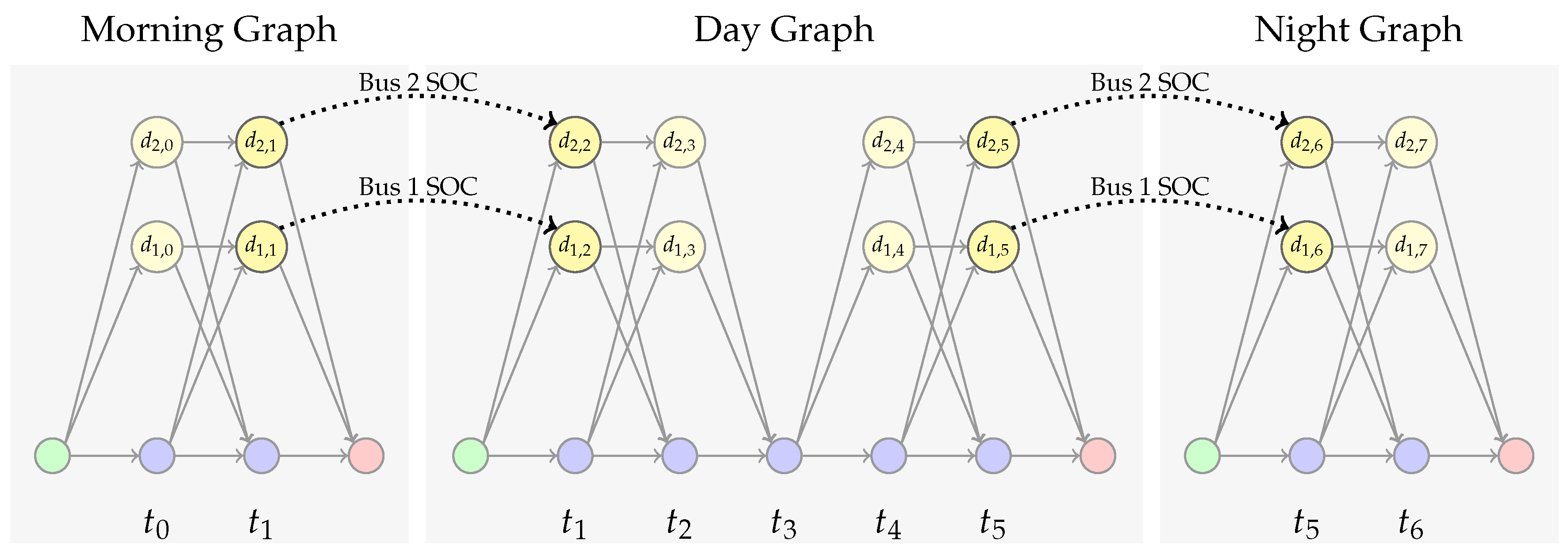
Each graph is connected by equating the appropriate SOC values. Consider the multi-graph formulation given in Figure 16. The morning graph is related to the day graph because $d_{1,1}$ and $d_{2,1}$ represent the same SOC values as $d_{1,2}$ and $d_{2,2}$, respectively. The same applies for the day and night graphs, where $d_{1,5}$ and $d_{2,5}$ represent the SOC values for $d_{1,6}$ and $d_{2,6}$. This equality relationship can be expressed as an equality constraint where

$$\begin{array}{c}\hfill {\mathbf{d}}_{\mathrm{graph}1}-{\mathbf{d}}_{\mathrm{graph}2}=\mathbf{0},\end{array}$$

(36)

or by

$$\begin{array}{c}\hfill D_{\mathrm{multi}-\mathrm{graph}}\mathbf{y}=\mathbf{0},\end{array}$$

(37)

where $D_{\mathrm{multi}-\mathrm{graph}}$ is an $\mathrm{nBus}\times \mathrm{nVar}$ matrix such that

$$\begin{array}{c}\hfill D_{\mathrm{multi}-\mathrm{graph}}\mathbf{y}={\mathbf{d}}_{\mathrm{graph}1}-{\mathbf{d}}_{\mathrm{graph}2}.\end{array}$$

(38)

Because all SOC values d are contained in $\mathbf{y}$, forming the matrix D amounts to placing 1 and $-1$ at the indices corresponding to $d_{\mathrm{graph}1}$ and $d_{\mathrm{graph}2}$, respectively, and zero otherwise.

6. Objective Function

The objective function in this work models the rate schedule used in [32], where the cost is modeled as the monthly charge a transit authority receives from the power provider. The objective function includes charges for energy, power, and facility use and implements both on- and off-peak rates.

The objective function also includes the effects and costs of uncontrolled loads. Uncontrolled loads might include the effects of patrons charging personal electric vehicles, electric trains passing through, CNG stations, etc. The loads used in this work were recorded at the UTA Intermodal Hub station in Salt Lake City (SLC), Utah, as the average power sampled at uniform time intervals.

6.1. Energy

Energy cost is assessed per kilowatt hour of energy consumed and includes the energy consumed by uncontrolled loads and bus chargers. Let $\mathbf{p}$ be the average external power used at each timestep, where ${\mathbf{p}}_i$ is the average power draw between $t_j$ and $t_{j+1}$. The energy consumed by external loads from $t_j$ to $t_{j+1}$ is computed as

$$e_j^l={\mathbf{p}}_i·{\Delta }_t,$$

(39)

where ${\Delta }_t$ is the change in time from $t_j$ to $t_{j+1}$ in hours. The energy consumed by bus chargers for the same interval is computed as

$$e_j^b=\sum _{k\in t}{g}_{i,k,l},$$

(40)

where $k\in t$ represents all values for g that took place between $t_i$ and $t_{i+1}$ for every bus. The total energy is computed as

$$e_j=e_j^l+e_j^b.$$

(41)

Equation (41) can be written in standard form as

$$\begin{array}{cc}\hfill e_j-\sum _{k\in t}{g}_{i,k,l}& =p_i·{\Delta }_t\hfill \\ \hfill \left[\begin{array}{ccc}{1}_{e_j}& -1_{g_1}& \dots -1_{g_n}\end{array}\right]\left[\begin{array}{c}{e}_j\\ g_1\\ ⋮\\ g_n\end{array}\right]& =p_i·{\Delta }_t.\hfill \end{array}$$

(42)

Because power providers charge different rates for the total power consumed during the respective on- and off-peak hours, Equation (42) is modified to reflect the energy consumed in arbitrary time periods. Let T be a set of $t_j$, or just j, which will later be used to denote on- and off-peak periods as $T_{\mathrm{on}}$ and $T_{\mathrm{off}}$. Equation (42) can be expanded to compute the total energy consumed in T as

$$\begin{array}{cc}\hfill e_T-\sum _{k\in T}{g}_{j,k,l}& =\left(\sum _{j\in T}{p}_j\right)·{\Delta }_t\hfill \\ \hfill \left[\begin{array}{ccc}{1}_{e_T}& -1_{g_1}& \dots -1_{g_n}\end{array}\right]\left[\begin{array}{c}{e}_T\\ g_1\\ ⋮\\ g_n\end{array}\right]& =e_T^{\mathrm{load}}.\hfill \end{array}$$

(43)

For multiple time periods, the constraint can be expanded in matrix form, where row i corresponds to the periods of time in $T_i$. Furthermore, by including the values for each $e_{T_i}$ in $\mathbf{y}$ and zero padding appropriately, the expanded form of Equation (43) can be written as

$$E\mathbf{y}={\mathbf{e}}^{\mathrm{load}},$$

(44)

where row i in E reflects Equation (43) for the time intervals in $T_i$, and ${\mathbf{e}}_i^{\mathrm{load}}$ contains the energy consumed by uncontrolled loads during $T_i$.

6.2. Power

Power costs are computed for the maximum average power draw, where the average is computed over a 15 min sliding window. The average power can be computed as the energy in the window divided by the window length in hours. In this case, a 15 min window equates to a quarter hour. Let ${\overline{p}}_j$ be the average power from $j-15$ to j. Equation (43) can be adapted to compute the average power as

$$\begin{array}{cc}\hfill {\overline{p}}_j-\left(\sum _{k\in T_j}\frac{1}{4}{g}_{i,k,l}\right)& =\left(\sum _{i\in T_j}{p}_i\right)·\frac{{\Delta }_t}{4}\hfill \\ \hfill \left[\begin{array}{ccc}{1}_{{\overline{p}}_j}& -\frac{1_{g_1}}{4}& \dots -\frac{1_{g_n}}{4}\end{array}\right]\left[\begin{array}{c}{e}_j\\ g_1\\ ⋮\\ g_n\end{array}\right]& =\frac{p_T·{\Delta }_t}{4}.\hfill \end{array}$$

(45)

Equation (45) can further be expanded and zero padded to compute the average power at each time, $t_j$ by applying Equation (45) to the corresponding window as

$$P\mathbf{y}=\mathbf{p}.$$

(46)

The maximum average power, denoted as $\widehat{p}$, is greater than or equal to each average power computed in Equation (46). This yields an additional set of inequality constraints

$$\begin{array}{cc}\hfill \left[\begin{array}{ccccc}-1_{\widehat{p}}& 1_{{\overline{p}}_0}& 0& \dots & 0\\ -1_{\widehat{p}}& 0& 1_{{\overline{p}}_1}& \dots & 0\\ -1_{\widehat{p}}& 0& 0& \dots & 1_{{\overline{p}}_j}\end{array}\right]\mathbf{y}& \le \mathbf{0}\hfill \\ \hfill P_{\max }\mathbf{y}& \le \mathbf{0}.\hfill \end{array}$$

(47)

Because the max average power is minimized in the objective function, the value for ${\widehat{p}}_{\max }$ will be forced down to the value of the greatest average power computed in Equation (46), and accurately reflect the maximum average power.

6.3. On/Off-Peak Rates

Power providers divide each day into on- and off-peak periods during which different rates are applied for both energy and power costs. Let H and L be the respective sets of all time indices in on- and off-peak periods, respectively. The cost of energy during on-peak hours can be expressed as

$$\begin{array}{cc}\hfill c_{{\mathrm{energy}}_H}& =\left(\sum _{j\in H}{e}_j\right)r_{e_{\mathrm{on}}}\hfill \\ \hfill & =\left[\begin{array}{ccccccc}{r}_{e_1}& 0& \dots & 0& r_{e_4}& \dots & 0\end{array}\right]\mathbf{y}\hfill \\ \hfill & ={\mathbf{r}}_{e_{\mathrm{on}}}^T\mathbf{y},\hfill \end{array}$$

(48)

where ${\mathbf{r}}_e^{\mathrm{on}}$ contains the value of $r_e^{\mathrm{on}}$ at the index corresponding to $e_j$ in $\mathbf{y}\forall j\in H$. A similar formulation can be used to describe the cost of energy consumed during off-peak hours.

An on-peak rate also applies to charges for power. Equation (47) can be adapted to only include rows that correspond to average power values during on-peak hours such that

$$\begin{array}{cc}\hfill \left[\begin{array}{ccccc}-1_{{\widehat{p}}_{\mathrm{on}}}& 1_{{\overline{p}}_0}& 0& \dots & 0\\ -1_{{\widehat{p}}_{\mathrm{on}}}& 0& 1_{{\overline{p}}_1}& \dots & 0\\ -1_{{\widehat{p}}_{\mathrm{on}}}& 0& 0& \dots & 1_{{\overline{p}}_j}\end{array}\right]\mathbf{y}& \le \mathbf{0}\hfill \\ \hfill P_{\mathrm{on}}\mathbf{y}& \le \mathbf{0}.\hfill \end{array}$$

(49)

Similarly, the off-peak max average power can be computed as

$$\begin{array}{cc}\hfill \left[\begin{array}{ccccc}-1_{{\widehat{p}}_{\mathrm{off}}}& 1_{{\overline{p}}_0}& 0& \dots & 0\\ -1_{{\widehat{p}}_{\mathrm{off}}}& 0& 1_{{\overline{p}}_1}& \dots & 0\\ -1_{{\widehat{p}}_{\mathrm{off}}}& 0& 0& \dots & 1_{{\overline{p}}_j}\end{array}\right]\mathbf{y}& \le \mathbf{0}\hfill \\ \hfill P_{\mathrm{off}}\mathbf{y}& \le \mathbf{0},\hfill \end{array}$$

(50)

where each row corresponds to ${\overline{p}}_j\forall j\in L$.

Many power providers include a facilities charge. The facilities charge is assessed per kW of the maximum average power and ignores on- and off-peak times. The total max average power is calculated using Equation (47).

The total power cost can be computed as the sum of the on-peak, off-peak, and facilities charges as

$$\begin{array}{cc}\hfill c_{\mathrm{power}}& =\left[\begin{array}{ccccccccc}{r}_{{\widehat{p}}_{\mathrm{on}}}& 0& \dots & 0& r_{{\widehat{p}}_{\mathrm{off}}}& 0& \dots & 0& r_{{\widehat{p}}_{\mathrm{facilities}}}\end{array}\right]\mathbf{y}\hfill \\ \hfill & ={\mathbf{r}}_{\widehat{p}}^T\mathbf{y}.\hfill \end{array}$$

(51)

6.4. Objective Function

The objective function combines the cost of energy and power, where the on-peak and off-peak energies are combined as

$$\begin{array}{cc}\hfill c_{\mathrm{energy}}& ={\mathbf{r}}_{e_{\mathrm{on}}}^T\mathbf{y}+{\mathbf{r}}_{e_{\mathrm{off}}}^T\mathbf{y}\hfill \\ \hfill & ={\left({\mathbf{r}}_{e_{\mathrm{on}}}+{\mathbf{r}}_{e_{\mathrm{off}}}\right)}^T\mathbf{y}\hfill \\ \hfill & ={\mathbf{r}}_e^T\mathbf{y}.\hfill \end{array}$$

(52)

The combined expression is given as

$$\begin{array}{cc}\hfill c_{\mathrm{total}}& =c_{\mathrm{power}}+c_{\mathrm{energy}}\hfill \\ \hfill & ={\mathbf{r}}_e^T\mathbf{y}+{\mathbf{r}}_{\widehat{p}}^T\mathbf{y}\hfill \\ \hfill & ={\left({\mathbf{r}}_e+{\mathbf{r}}_{\widehat{p}}\right)}^T\mathbf{y}\hfill \\ \hfill & ={\mathbf{r}}^T\mathbf{y}.\hfill \end{array}$$

(53)

Equation (53) is used as the objective function in a mixed-integer linear program of the form

$$\begin{array}{cc}\hfill & \underset{\mathbf{y}}{\min }{\mathbf{r}}^T\mathbf{y}\mathrm{subject}\mathrm{to}\hfill \\ \hfill & C_{\mathrm{eq}}\mathbf{y}={\mathbf{c}}_{\mathrm{eq}},C_{\mathrm{ineq}}\mathbf{y}\le {\mathbf{c}}_{\mathrm{ineq}},\hfill \end{array}$$

(54)

where $C_{\mathrm{eq}},{\mathbf{c}}_{\mathrm{eq}},C_{\mathrm{ineq}}$, and ${\mathbf{c}}_{\mathrm{ineq}}$ are formed by stacking the equality and inequality constraints from Equations (6), (11), (35), (46), (47), (49), and (50),

$$\begin{gathered} \underset{\mathbf{y}}{\min }{\mathbf{r}}^T\mathbf{y}\mathrm{subject}\mathrm{to} \\ \left[\begin{array}{c}\begin{array}{c}\tilde{A}\hfill \end{array}\hfill \\ D_{\mathrm{eq}}\hfill \\ P\hfill \end{array}\right]\mathbf{y}=\left[\begin{array}{c}{\mathbf{c}}_f\hfill \\ {\mathbf{d}}_{\mathrm{eq}}\hfill \\ \mathbf{p}\hfill \end{array}\right],\left[\begin{array}{c}\tilde{B}\hfill \\ D_{\mathrm{ineq}}\hfill \\ P_{\max }\hfill \\ P_{\mathrm{on}}\hfill \\ P_{\mathrm{off}}\hfill \end{array}\right]\mathbf{y}\le \left[\begin{array}{c}\mathbf{1}\\ {\mathbf{d}}_{\mathrm{ineq}}\\ \mathbf{0}\\ \mathbf{0}\\ \mathbf{0}\end{array}\right]. \end{gathered}$$

(55)

7. Results

This section discusses the results for applying the proposed method at the Utah Transit Authority station in Salt Lake City, Utah, (UTA). The UTA currently maintains a day-charging station located at a central bus depot, which serves as the singular charge point for BEBs and contains a limited number of “Fast-Chargers”. At night, each BEB is taken to a stall, where the BEB is connected to a “slow-charger”. We collected historical data that provide insight into the external loads which are present on the grid during a 24 h period, and introduced these data as a model for the “Uncontrolled Loads”. We are particularly interested in observing performance as the number of day chargers become scarce because their installation requires a significant financial investment. Furthermore, UTA also plans to increase their fleet size, and so we also look to see how the monthly cost of energy scales as the fleet size increases. We also compare the proposed method against two other charging paradigms. The first models how a traditional bus driver might behave in the absence of a centralized coordinator, and the second is an optimization solution from the current literature, which focuses on minimizing the instantaneous load on the grid. This section contains the results of the planning framework and is subdivided into three subsections: uncontested results, contested results, and multi-rate comparisons.

7.1. Baseline and Setup

The experiments in this section compare the results of the framework given in Equation (55) with a baseline that models the general behavior of bus drivers at the Utah Transit Authority (UTA) in SLC, Utah and the planning framework from [29]. All methods use a MILP to find an optimal solution and are solved up to a 2% gap using Gurobi [38]. Model parameters such as $\delta$, arrival, and departure times were computed from historical data provided by UTA.

According to UTA, bus drivers generally charge whenever possible. Our baseline scenario reflects this default bus driver behavior using an objective function that maximizes the number of charging instances, which is computed as the sum of group flow values, resulting in the objective function

$$\underset{\mathbf{y}}{\max }{\mathbf{1}}^{T}B\mathbf{y},$$

(56)

All other constraints are the same, which results in the baseline formulation

$$\begin{gathered} \underset{\mathbf{y}}{\max }{\mathbf{1}}^{T}B\mathbf{y}\mathrm{subject}\mathrm{to} \\ \left[\begin{array}{c}\begin{array}{c}\tilde{A}\hfill \end{array}\hfill \\ D_{\mathrm{eq}}\hfill \\ P\hfill \end{array}\right]\mathbf{y}=\left[\begin{array}{c}{\mathbf{c}}_f\hfill \\ {\mathbf{d}}_{\mathrm{eq}}\hfill \\ \mathbf{p}\hfill \end{array}\right],\left[\begin{array}{c}\tilde{B}\hfill \\ D_{\mathrm{ineq}}\hfill \\ P_{\max }\hfill \\ P_{\mathrm{on}}\hfill \\ P_{\mathrm{off}}\hfill \end{array}\right]\mathbf{y}\le \left[\begin{array}{c}\mathbf{1}\\ {\mathbf{d}}_{\mathrm{ineq}}\\ \mathbf{0}\\ \mathbf{0}\\ \mathbf{0}\end{array}\right]. \end{gathered}$$

(57)

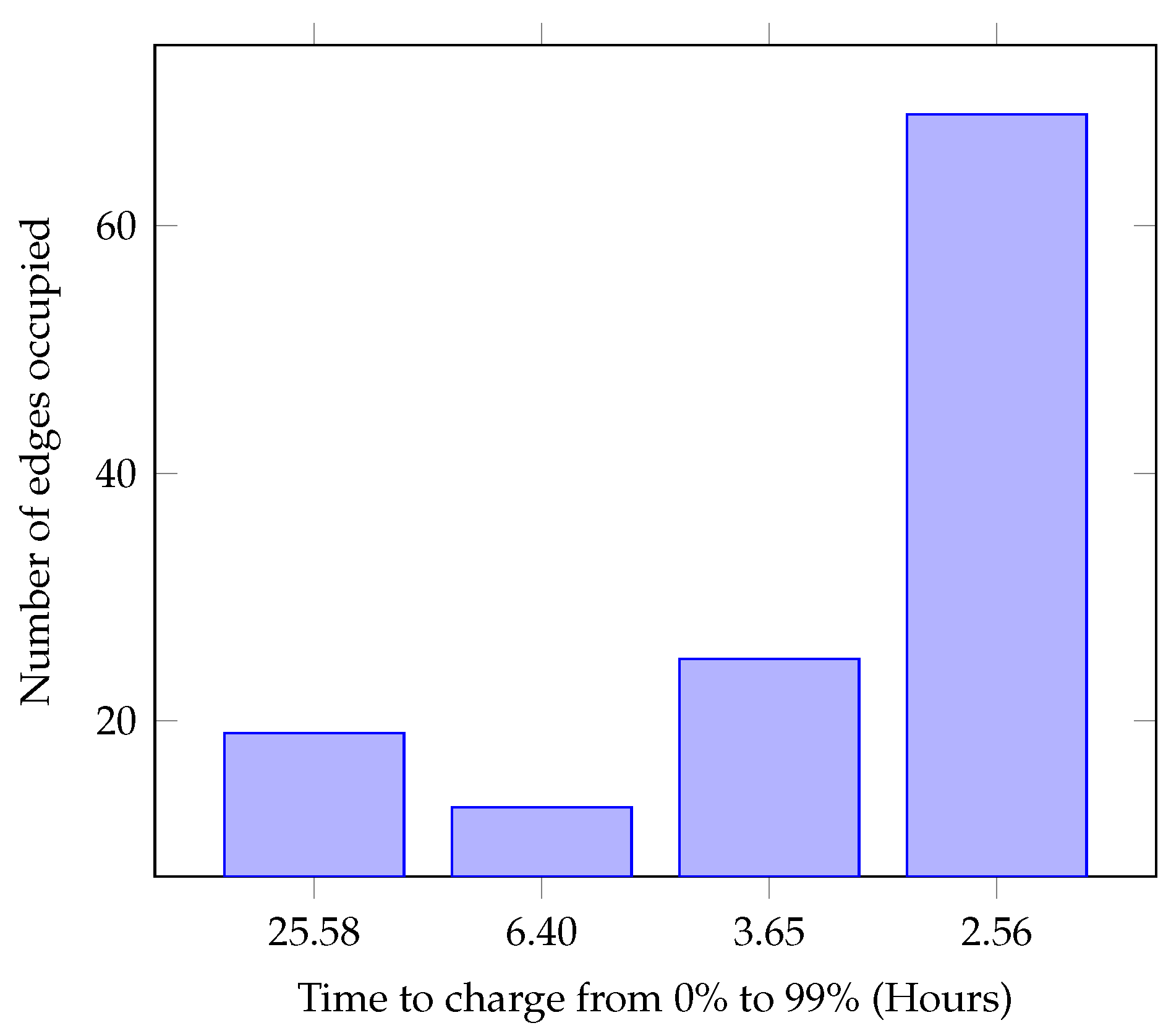
Each experiment is run using a five minute timestep such that the time difference between $t_k$ and $t_{k+1}$ is five minutes. Four charge rates are used during the following experiments: ${\overline{a}}_1=0.9851$, ${\overline{a}}_2=0.9418$, ${\overline{a}}_3=0.9003$, and ${\overline{a}}_4=0.8607$. Each value for $\overline{a}$ represents a different charge rate and is referenced by how much time it would take a bus to charge from 0% to 99%. For the rates used in the following set of experiments, a bus would need 25.58 h to charge from 0% to 99% with ${\overline{a}}_1$, 6.4 h with ${\overline{a}}_2$, 3.65 with ${\overline{a}}_3$, and 2.56 with ${\overline{a}}_4$.

Night charging uses a single charge rate of ${\overline{a}}_1$ for all experiments. Experiments with single-rate day charging use ${\overline{a}}_4$, and multi-rate experiments incorporate four charge options: ${\overline{a}}_1$, ${\overline{a}}_2$, ${\overline{a}}_3$, and ${\overline{a}}_4$.

Uncontrolled loads are modeled with data from the TRAX Power Substation (TPSS) at the UTA Intermodel Hub site in Salt Lake City. It is also assumed that each bus starts and ends each day with an SOC of $80\%$ and has a maximum charge capacity of 100 kWh.

7.2. Uncontested Results

This section explores performance in a scenario where there is one charger per bus during the day, making charge resources uncontested. The optimal charge schedule associated with Equation (55) is compared with the schedule developed by the baseline in Equation (57). The total monthly cost is computed using the rates given in Rocky Mountain Power Schedule 8 and is computed in Equation (58):

$$\begin{array}{cc}\hfill \cos \mathrm{t}=& \mathrm{facilitiesPower}·4.81+\mathrm{onPeakPower}·15.73+\hfill \\ \hfill & \mathrm{onPeakEnergy}·0.058282+\mathrm{offPeakEnergy}·0.029624\hfill \end{array}$$

(58)

There is also a customer service charge of $71.00$ in the rate schedule, but because the service charge does not depend on a customer’s behavior, it is ignored.

Because Equation (58) is driven by facilities power, on-peak power, on-peak energy, and off-peak energy, these four criteria are used to evaluate the optimal and baseline charge plans. Furthermore, because the on- and off-peak energy charges contribute little to the cost differences, they are grouped together for comparison.

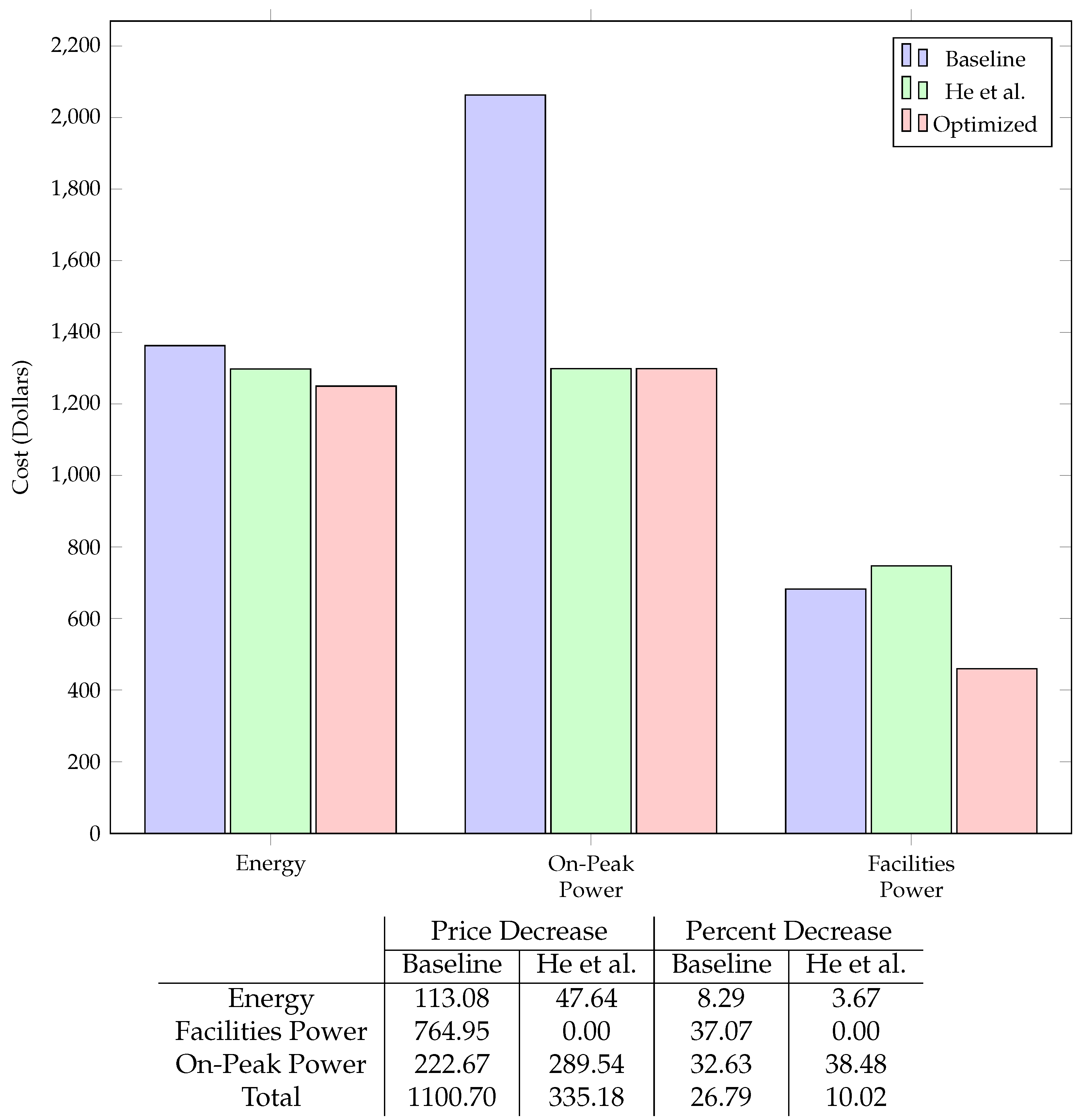
Figure 17 compares the cost of energy, on-peak power, and facilities power for the baseline [29], and this work’s scheduling strategies. Note how the schedule given by He et al. [29] is similar in both energy costs and on-peak power charges but is more expensive in the facilities charge. These differences are expected, as He et al. [29]. minimize the cost of energy by charging during off-peak periods. Because there is minimal charging during on-peak times, the on-peak power charges reflect the uncontrolled loads and are therefore the same. The differences in facilities is present because He et al. do not include the overall maximum average power in their framework.

Additionally, the facilities and on-peak power costs for the baseline schedule are significantly larger than the optimized schedule. To better understand the cost disparity, we observe the load profiles to identify how the optimized schedule avoids the costs incurred by the baseline.

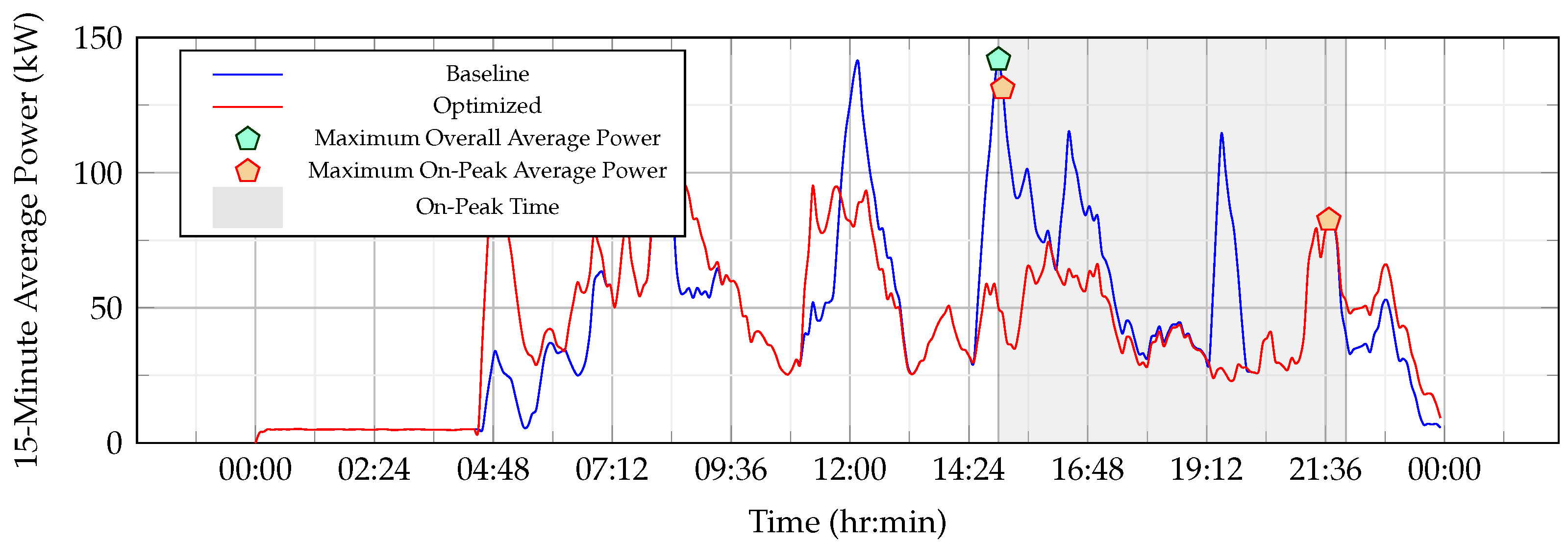
Figure 18 shows the 15 min average power for both the baseline and optimal schedules. Note how the optimal schedule incurs a lower average power for both on- and off-peak time intervals. The reduction in average power is what leads to the cost disparity between the on-peak and facilities power costs in Figure 17.

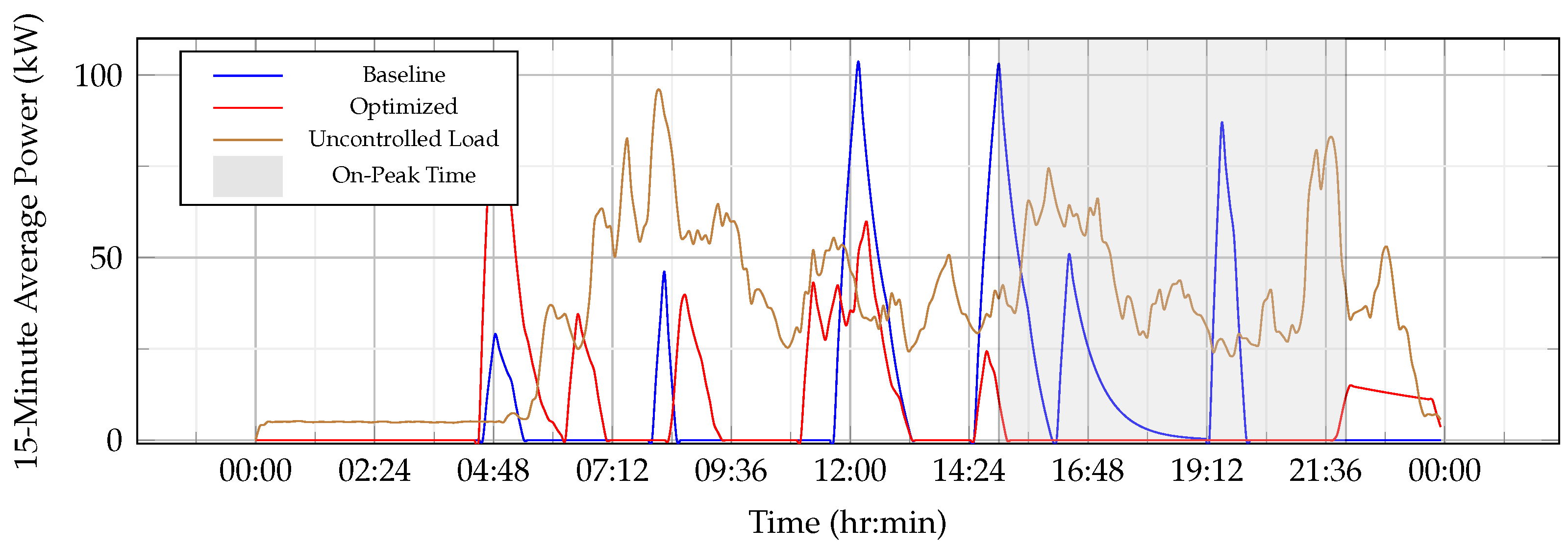
The underlying behavior can be observed in Figure 19, which separates the loads into their controlled and uncontrolled constituents. Because the uncontrolled loads are shared between both scenarios, Figure 19 shows the 15 min average power for uncontrolled, optimal charging, and baseline charging loads.

Observe how the optimized schedule avoids charging during on-peak hours and regulates each charge event to spread the power draw over larger periods of time. Furthermore, bus charging is avoided when uncontrolled loads are high, resulting in a reduced 15 min average power. Reducing the average power and not charging during on-peak periods results in the dramatic cost reduction shown in Figure 17.

7.3. Contested Results

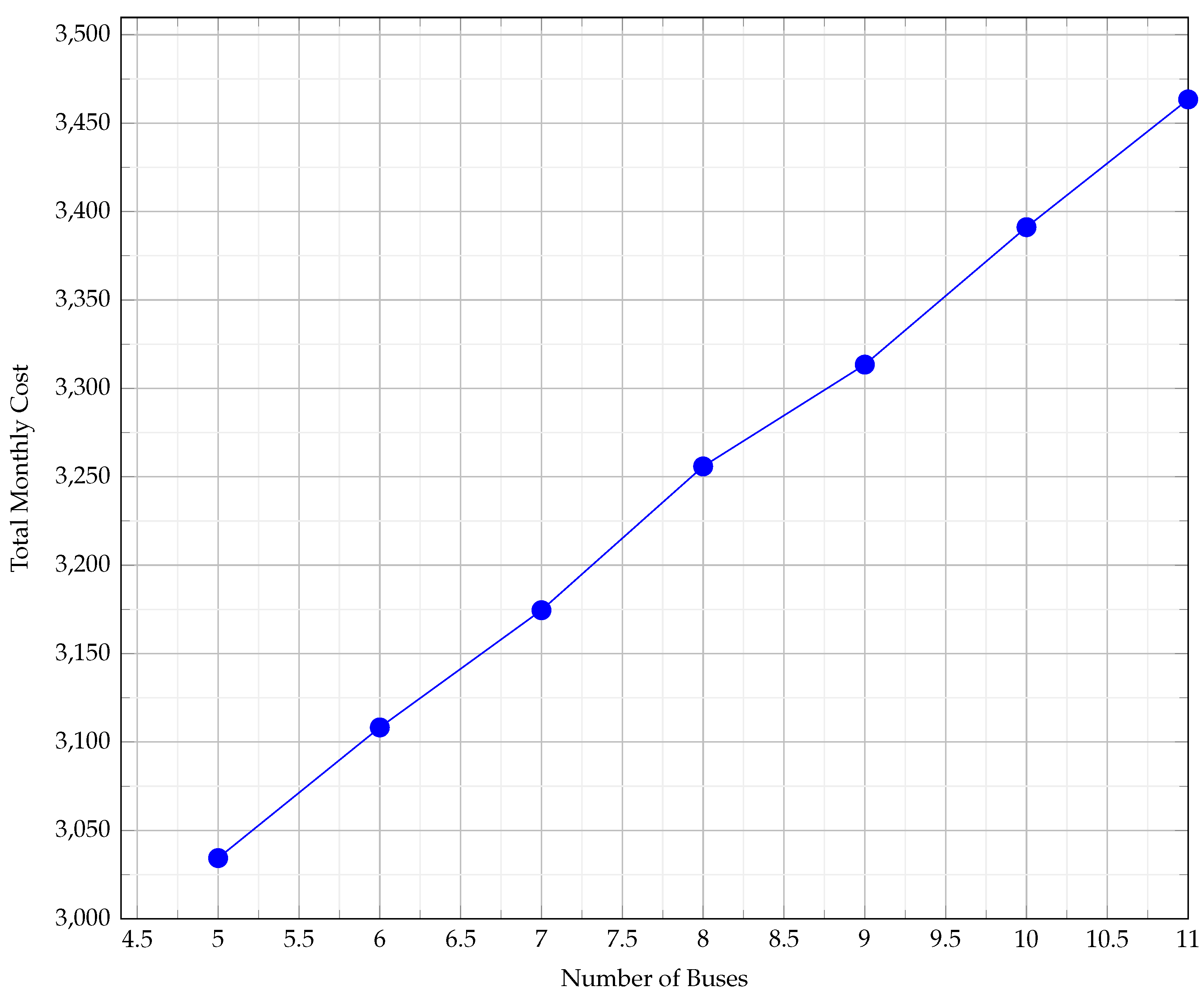
This section observes the performance of the optimal schedule as charge resources become scarce, creating a contested environment. Resource contention is most prevalent when chargers are scarce and pushes buses to charge in non-ideal circumstances. For example, if charging resources are saturated during off-peak hours, other buses might be forced to charge in the on-peak window. The impact of contention is measured as the change in monthly cost when the number of chargers is held constant and the number of buses increases.

In this analysis, one charger is used, and the number of buses is varied from five to eleven. Figure 20 shows the monthly cost as a function of the number of buses. Note the minimal cost increase per bus, where each successive bus costs around USD $75.00$, which approaches the cost of energy that is required to provide transit services. Because the additional cost per bus is roughly the cost of energy, there are no additional facilities and on-peak power charges, showing that optimal charge plans also minimize cost in the presence of contention.

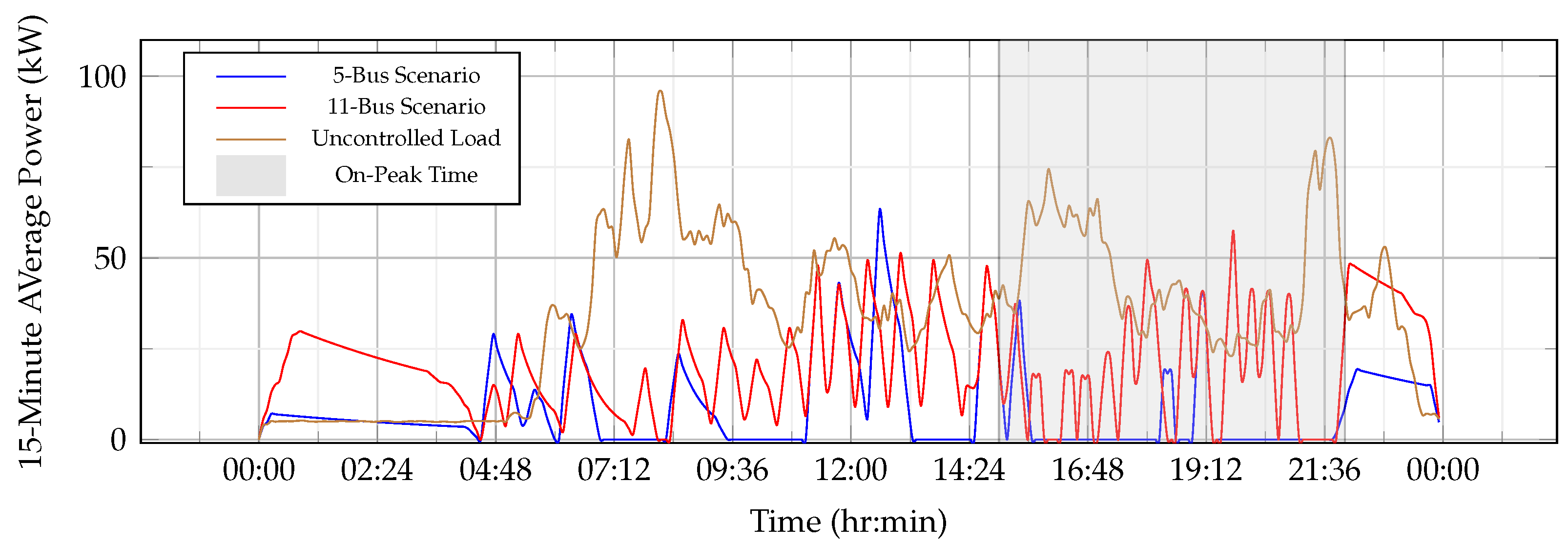
We desire to know how this is achieved. Figure 21 shows the 15 min average power for controlled and uncontrolled loads for a five-bus and eleven-bus scenario. In the 5-bus scenario, loads are easily distributed amongst off-peak hours, resulting in an optimized cost. The 11-bus scenario requires significantly more power and is forced to charge during on-peak hours. Note, however, that the average power is kept relatively low, and the additional charge sessions never cause the average power to supersede the maximum average power of the uncontrolled loads. Both scenarios also make ample use of night charging, where the number of chargers is the same as the number of buses.

7.4. Multi-Rate Comparison

This subsection compares a multi-rate and single-rate charge schedule. The multi-rate schedule includes $a_1$, $a_2$, $a_3$, and $a_4$ as defined in Section 7.1. The single-rate schedule assumes the static charge rate associated with $a_1$. Two scenarios are considered. The first compares the cost of multi- and single-rate plans for a 5-bus 1-charger scenario. The second compares performance for a 35-bus 6-charger scenario.

The potential savings for using a variable charge rate in a 5-bus 1-charger scenario are found to be negligible. The cost of the multi-rate scenario is USD 3006.94, and the cost of the single-rate scenario is USD 3007.77, which gives a total savings of USD 0.83. A 36-bus 6-charger comparison also yields minimal cost savings.

While examining the most commonly used edges, we observe that edges corresponding to a maximum charge rate are used most frequently as shown in Figure 22, which explains the similarities in cost. If the highest rate is almost always selected, the resulting plan would resemble a single-rate schedule, resulting in a singe-rate cost.

Another explanation for the cost similarity is found in how monthly cost is computed. Because the monthly cost is based on the average instantaneous power, both high and low charge rates can give the same results over a fixed time period. The charge schedules shown in both single and multi-rate plans charge buses in relatively small time periods. Fast charging over small periods of time is equivalent to slow charging over longer periods. In this way, the average power can be kept low even when using high charge rates (see Figure 20 and Figure 21).

8. Conclusions and Future Work

In conclusion, the charge schedules developed in Equation (55) yield significant cost savings over both the baseline and the work by [29]. These savings come from minimizing the average power consumption and charging during off-peak hours. Cost savings are maintained in both uncontested and resource-constrained scenarios. There is also little to be gained by offering multiple charge rates because the average power can be managed with high charge rates by reducing the charge duration. Furthermore, it was shown that when given the choice, the optimizer primarily selected high charge rates, which reduces the problem complexity to the single-rate formulation.

In practice, this work demonstrates the feasibility of large-scale BEB conversion with a small number of charging resources. Furthermore, the monthly cost can be made linear with the number of buses so that BEB conversion is scalable even when the number of fast-charging resources is relatively small and the grid is shared with other significant power users. In practice, accommodating other power users allows the transit authority to aggregate their meters, which decreases the cost of the charging infrastructure for power providers and the monthly cost for transit authorities.

Although multi-rate charging does not significantly reduce the monthly cost, it could be useful in prolonging battery life. The high power rates observed in this work can reduce the lifespan of the battery, whereas lower charge rates can prolong battery life. Therefore, future work incorporating battery health will be explored. We believe that multi-rate charging may offer some flexibility in this scenario. Future work will extend the discrete charge levels in this work to a continuous rate selection.

Because this work presents only a planning framework for a global solution over large stretches of time, it is computationally infeasible to recompute when unplanned events occur. Future work could move this framework toward real-time deployment using a hierarchical approach to control the charging. A precomputed global plan supports the real-time planner by providing top-level guidance. The lower-level real-time planner will adapt to unplanned events by controlling for a return from the current state to the global plan over a finite sliding horizon.

Finally, the computational complexity of our approach decreases as the number of chargers increase but suffers when planning for large bus fleets, as the number of constraints and solution variables scales linearly with the number of buses as shown in Figure 23. Future improvements might use a solution from a heuristic approach as a “warm start” for the optimizer, which would reduce the computational complexity of finding a globally optimal solution.

In summary, the proposed work could be extended in the following areas: (1) Decrease the compute time by computing a “warm start” for the optimizer using a heuristic approach. (2) Incorporate renewable energy into the optimization scheme in the same way the uncontrolled loads were used. (3) Account for variability in the uncontrolled loads by modifying the inputs to reflect worst-case scenarios. (4) Include the projected costs of battery replacement as a function of high charge rates.